A multiscale finite element technique for nonlinear multi-phase materials

This is a repository copy of

A multiscale finite element technique for nonlinear multi-phase

materials

.

White Rose Research Online URL for this paper:

http://eprints.whiterose.ac.uk/88044/

Version: Accepted Version

Article:

Molina, A.J.C. and Curiel-Sosa, J.L. (2015) A multiscale finite element technique for

nonlinear multi-phase materials. Finite Elements in Analysis and Design, 94. 64 - 80. ISSN

0168-874X

https://doi.org/10.1016/j.finel.2014.10.001

[email protected]

Reuse

Unless indicated otherwise, fulltext items are protected by copyright with all rights reserved. The copyright exception in section 29 of the Copyright, Designs and Patents Act 1988 allows the making of a single copy solely for the purpose of non-commercial research or private study within the limits of fair dealing. The publisher or other rights-holder may allow further reproduction and re-use of this version - refer to the White Rose Research Online record for this item. Where records identify the publisher as the copyright holder, users can verify any specific terms of use on the publisher’s website.

Takedown

If you consider content in White Rose Research Online to be in breach of UK law, please notify us by

A multiscale finite element technique for nonlinear multi-phase materials

A.J. Carneiro Molinaa_{, J.L. Curiel-Sosa}b∗

a

Rockfield Sofware Ltd, Ethos, Kings Road, Swansea Waterfront, SA1 8AS, UK. b

Department of Mechanical Engineering, University of Sheffield, Sir Frederick Mappin Building, Sheffield S1 3JD, UK.

Abstract

This paper presents a multiscale finite element homogenization technique (MFEH) for mod-elling nonlinear deformation of multi-phase materials. A novel condensation technique to relate force variations acting on the representative volume element (RVE) –involving antiperiodicity of traction forces at RVE corners– and displacement variations on boundary-nodes is proposed. The formulation to accommodate the condensation technique and overall tangent modulus is presented in detail. In this context, the effective homogenized tangent modulus is computed as a function of microstructure stiffness matrix which, in turn, depends upon the material properties and, geo-metrical distribution of the micro-constituents. Numerical tests concerning plastic materials with different voids distributions are presented to show the robustness of the proposed MFEH.

Keywords: Finite Element Method (FEM), Voids, Plasticity, Multiscale, homogenisation, condensation technique

1. Introduction

The heterogeneous nature of materials has a significant impact on the observed macroscopic behaviour of multi-phase materials. Their properties depend upon the size, shape, spatial distribu-tion and material parameters of micro constituents and their respective interfaces. For instance, in reinforced composites, stiff and strong phase inclusions of glass, graphite, boron, or aluminium ox-ide, are added to epoxy resin, steel, titanium, or aluminium matrices to enhance strength, thermal expansion coefficient and wear resistance of structures.

A transition from the microscopic properties to their macroscopic counterparts based on an averaging principles is termed homogenization. The simplest method leading to homogenized mod-ulus of heterogeneous material is based on the rule of mixture. This approach takes only one microstructural characteristic into consideration: the volume ratio of the heterogeneities. A more sophisticated method is the effective medium approximation, as established by Eshelby [1] and further developed by Hashin [2], Mori and Tanaka [3] and more recently by Nan and Clarke [4].

Although some work has been done on extension of the self-consistent approach to non-linear cases, significantly more progress in estimating advanced properties of composites has been achieved by variational bounding methods (see [5, 6]). The variational bounding methods are based on suitable variational (minimum energy) principles and provide upper and lower bounds for the overall properties of the composite. Another approach is based on mathematical Asymptotic Expansion Homogenization (AEH) theory, [7, 8, 9]. AEH is a perturbation technique based on the asymptotic series expansion in ε, a scale parameter of a primary variable. The scale parameter is a ratio between the length scales, represented by the relation between micro heterogeneities size and a measure of macrostructure. It is represented by a very small positive number ε = _Ll _≪ 1, see [10, 11, 12, 13]. The asymptotic homogenization technique gives effective overall properties plus local stress and strain values. However, the considerations are restricted to very simple microscopic geometries and simple material models, mostly at small strains.

The unit cell methods represent another way to approach the analysis of multi-phase materials. They appeared due to the complexity of microstructural mechanical and physical behaviour along with the developments of computational techniques. These approaches have been used in a large number of applications, see [14, 15, 16, 17, 18]. The unit cell methods provide information on the local microstructural fields and effective material properties. Once the constitutive behaviour be-comes nonlinear, it is extremely difficult to make assumption on a suitable macroscopic constitutive format, see [19, 20, 21].

Most of the homogenization techniques aforementioned are not suitable for finite deformations or complex loading paths, since they do not account for geometrical and physical changes in the microstructure. In the Finite Element Method (FEM), the use of a single element capturing all microstructural details in a numerical solution of macroscopic BVP becomes impractical. An alter-native approach for homogenization of multi-phase heterogeneous materials, known asMulti-Scale Computational Homogenization or Micro-Macro Modelling has been gaining considerable popular-ity in the computational mechanics circles. Since the basic principles for the micro-macro modelling of heterogeneous materials were introduced (see [22, 11, 23, 24, 25]), this technique has proved to be the most effective way to deal with arbitrary physically non-linear and time dependent mate-rial behaviour at micro-level. A number of recent works deal with various approaches and tech-niques for the micro-macro simulation of heterogeneous materials. Among these, the contributions [26, 27] are highlighted for analysis of polycrystalline materials. The multiscale modelling tech-niques above do not lead to closed-form overall constitutive equations. However, they compute the stress-deformation relationship at every macro point of interest by modelling of the microstructure RVE corresponding to the macroscopic point. The advantages of multiscale techniques are the following:

• They enable the incorporation of finite deformations and rotations at both micro and macro levels.

• They are suitable for nonlinear material behaviour.

• They provide the possibility to introduce detailed microstructural information, including ge-ometrical and physical evolution, into the macroscopic analysis.

• Although our study is confined to the finite element method, they allow any modelling tech-nique on the micro level.

The main disadvantage of multiscale techniques is the high computational cost. This concern however can be overcome partially by parallel computation, see [28] for further details on this.

Herein, two of the forces in one node representing antiperiodic traction are condensed. This approach leads to an innovative treatment of the problem. The paper is structured as follows: Firstly, the necessary background is presented. Secondly, the novel condensation technique, associ-ated tangent modulus, etc are described and formulation is developed in detail. Finally, numerical tests are presented and compared with other results from the literature.

2. Macroscale and microscale

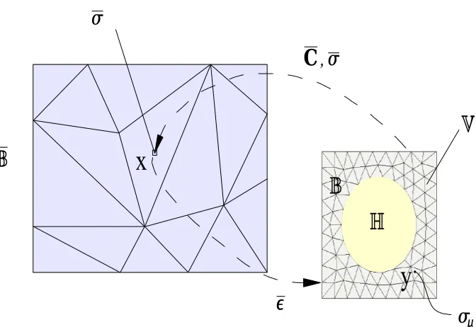
A homogenized macro-continuum with locally attached microstructures is considered herein. The microstructure is denoted by B _⊂ R3 _{with overall properties related to the macrocontinuum} B_⊂R3_.

A point x ∈ B of the homogenized macromedium B ⊂ R3 is represented as a microstructure

B _⊂ R3_{. The tensors σ and σµ denote the macro and micro Cauchy stress tensor at x ∈} B _and

y ∈ B, respectively. The Representative Volume Element (RVE) of the microstructure V ⊂ R3

represents the part of the heterogeneous material consisting of the solid partB_{and the hole} H_{, i.e.} V₌B_∪H _{and ∂}B_=∂V_∪∂H_{. It is assumed the traction field on the surface of the holes in the}

interior of RVE vanishes, i.e.

t(y, t) =0 at y ∈∂H (1)

wheret_≡σµ·n on∂Bis the traction field vector on the surface with outward normaln aty ∈∂B.

A discrete model of the macro and microstructure is considered in Figure 1. The overall macro-scopic deformationǫis prescribed over the discretised RVE. The main idea of this procedure is based on finite element (F.E.) discretisation. At every integration Gauss point of the macrostructure, a discrete RVE microstructure is considered as representation of the macro Gauss point. Based on the Finite Elements discretisation of the microstructure, the goal is to develop a procedure for computing the overall tangent modulus C _{and macroscopic average stress σ at each macroscopic}

Figure 1: Micro to macro transition

3. Displacement field partition and matrix notation

The displacement field is divided into two parts u =u∗

+ue whereu∗

is the so-called Taylor displacement which is expressed in its discrete form as,

u∗

j ≡ ǫyj j = 1· · ·n (2)

for the n nodes of the microstructure RVE. The displacement fluctuation u_e is the unknown for every node of the discretised microstructure unit cell.

Henceforth, standard Finite Element matrix notation will be used, where the tensor entities so far used, can be identified now in the form

ǫ _≡

 

 ε11

ε22 2ε12

 

 and uj ≡

u1

u2

j

(3)

withǫ as matrix representation of macrostrain tensor anduj is the displacement field at node j of the discretised unit cell V_{.Moreover, the averaged stress fieldσ and the force vectorfjassociated}

with the microcell node j, are also defined in this notation as follows,

σ _≡

  

σ11

σ22

σ12

 

 and fj ≡

f1

f2

j

The Taylor displacement u∗

j of the node j is computed in the following matrix form

u∗

j = DTj ǫ, j = 1· · · n. (5)

whereD_{j is the} coordinate matrix at node j of the microstructure is defined as,

D_{j ≡} 1

2

 

2y1 0 0 2y2

y2 y1

 

j

(6)

4. Discretised micro-equilibrium state and solution procedure

A procedure based in a Newton-Raphson scheme is given to find the equilibrium at the mi-crostructure RVE at time step n+ 1 assuming the system is already in equilibrium at time step

n. The general idea consists in taking the microstructure as ’frozen’ with macroscopic strain

ǫ = constant. Therefore, the variation of the Taylor displacement is zero during the iteration du∗

=0, because it is applied at the beginning of the process.

Before proceeding with description of the scheme, the incremental displacement field _△u =

un+1−uncan be additively decomposed thanks to the additive properties of the strain tensorǫas

follows,

△u=_△u∗

+_△ue=_△ǫy+_△ue (7)

where _△u∗

is the incremental Taylor displacement and _△ue is the incremental displacement fluctuation. The general solution procedure is described as follows:

1. The initial incremental displacement guess _△u0 _{is given as the incremental Taylor} displace-ment,

△u0 =_△u∗

=_△ǫy (8)

In other words, the incremental macro strain _△ǫ is fully prescribed at the first pseudo step, so that, the Taylor displacement is fully prescribed as the initial guess. This means that the initial displacement guess at time step n+ 1, u0_n+1, is given by,

u0_n+1=un+△u0 (9)

Using the split displacementu =u∗

+euat time stepn, the initial guess displacement is then expressed as,

u0_n+1 =u∗

n+1+uen (10)

In the above it can be observed that the incremental Taylor displacement_△u∗

taken as the converged from the previous time step n. Therefore, eu0_n+1 =uen or in another

words the incremental fluctuation is zero during the initial guess _△u_e= 0

2. Computation of the internal forcesfint. This is computed with the incremental displacement △u and the set of state variables_{En+1,αn+1} at microscopic Gauss point level.

3. Check convergence_kr_k< εtolerance. This residual forcerdepends on the boundary constraint

applied on the RVE.

• IF_kr_k< εtolerance. EQUILIBRIUM. The solution is ukn+1. END OF ITERATION • ELSE GO TO NEXT STEP

4. Computation of the incremental internal fluctuation. Let assume that the differential fluctu-ation is divided in two parts,

δeu=

δ_eur δued

(11) where δu_er are the independent d.o.f. andδeud are the dependent d.o.f. displacements of the

microstructure. Thereforeδued is known once δeur is computed. They are different depending

on the micro boundary constraint ( Linear or Periodic b.c. ). The Newton-Raphson iteration is defined by,

Kr δeur =−r → δuer=−K

−1

r r (12)

whereris the residual force andKris the reduced matrix of the system. In Sections 6.5 and 7.7

particularisations for Linear and Periodic b.c. are given, respectively.

The updating of the incremental fluctuation is_△ue _{← △}u_e+δue and the incremental displace-ment_△u _{← △}u+δue

GO TO step 2.

Finally, when the microequilibrium is reached, the macro Cauchy stressσn+1is computed from the value of the boundary forces. This macro stress is used to compute the internal forces at the macro level.

5. General average stress and overall tangent modulus computation

5.1. Average stress computation

Assuming no body forces in the expression for the average stress, in the discrete setting,tdA_→ fext_j , that is the infinitesimal force t dA becomes the finite forcefext_j at nodal position y_j on the boundary∂V_{. Therefore, the average stress degenerates into the discrete sum}

σ = 1 |V_|

nb X

j = 1

sym[fext_{j ⊗}y_j] (13)

σ = 1 |V_|

nb X

j = 1

D_j fext_j (14)

where D_{j is the coordinate matrix (6) evaluated at node j on the boundary of the discretised}

microstructure RVE∂V_{. The above expression can be rearranged in the following global expression}

σ = 1 |V_| Db f

ext

b , (15)

where fext_b is the external nodal force vector of the boundary nodes, and D_{b is the} boundary coor-dinate matrix defined byD_{b ≡}Db₁ Db_{2 . . .} Db_n

b

.

5.2. Overall tangent modulus computation

In the computational homogenization approach no explicit form of the constitutive behavior on the macro-level is assumed a priori, so that the tangent modulus has to be determined numerically by relations between variations of the macroscopic stress and variations of the macroscopic strain at such integration macro Gauss point. This can be accomplished by numerical differentiation of the numerical macroscopic stress-strain relation, for instance, by using forward difference approxima-tions as suggested in [27]. Another approach is to condense the microstructural stiffness matrix to the macroscopic matrix tangent modulus. This task is achieved by reducing the total RVE system of equations to the relation between the forces acting on the boundary∂V _{and the displacement}

on the boundary. The innovative modelling of the anti-symmetry traction vectors at the nodes at the corners leads to a nonconventional condensation, obtaining a novel effective macroscopic tan-gent modulus. It is a direct condensation to obtain a relation between the variation of the forces acting on the boundary (∂V_{) and the variation of the Taylor displacement on the boundary nodes}

(du∗

), which depends linearly of the macroscopic strain (dǫ). The total microstructural system of equations that gives the relation between the iterative nodal displacement du and iterative nodal external force vectors is

K du= dfext. (16)

With the displacement partition u =u∗

+eu the system can be rearranged as follows,

Kdu= dfext _⇒Kdu∗

+Kdue= dfext

The boundary constraints are then applied to this system in the following sections to condense the system. This procedure gives the expression that relates the variation boundary external forces df_bextagainst the variation of the Taylor displacement du∗

.

C ₌ dσ

dǫ =

1 |V_| Db

df_bext

dǫ (17)

Particularisations of the computation of average macrostress and overall tangent modulus are given for Taylor assumption, Linear b.c. and Periodic b.c. below.

6. Discrete form of the linear displacements boundary condition

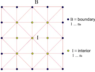
In view of the discrete formulation of the boundary conditions outlined, the nodes of the mesh are partitioned into those on the surface ∂V _{of RVE and those in the interior of} V_{, see Figure 2.}

In this mesh nb boundary nodes and ni internal nodes are distinguished.

Figure 2: Mesh for linear displacement on the boundary

6.1. Partitioning of algebraic equations

Partitioning of the current nodal displacements and nodal forces is given as,

u=

ui

ub

≡

L_iu L_bu

and f =

fi

fb

≡

L_if L_bf

(18)

Here L_{i and} L_{b are the connectivity matrices, which define the interior contribution and the}

con-tributions of the boundary nodes, respectively. These are Boolean matrices, i.e. they consist of integers 0 and 1. Displacements ui and ub are gathered fromu. Using these two vectors, a new u is obtained as shown in (18).

In line with (18), the tangent stiffness matrix is rearranged as

K= df

int

du =

kii kib

kbi kbb

≡

L_iKLT

i LiKLTb

L_bKLT_i L_{b K}LT

b

(19)

6.2. Linear displacement

At each node j of the boundary ∂V _{condition induces the discrete constraint, uej = 0 j =}

1 _{· · ·}nb. These constraints can be represented as a global boundary displacement vectorueb = 0. Following matrix notation, the global coordinate matrix is defined as follows,

D_{global,l ≡}D_i D_{b,l (20)}

where D_{i and} D_{b,l are the} interior coordinate matrix and the boundary coordinate matrix, respec-tively, given as

D_{i ≡}Di₁ Di_{2 . . .} Di_n

i

and D_{b,l ≡}Db₁ Db_{2 . . .} Db_n

b

. (21)

The matricesD_{i and} D_{b,l are defined in terms of node coordinate matrices (6) for the interior and}

boundary nodes, respectively. The Taylor displacementu∗

previously defined inu∗ = DT

globalǫfor the Taylor assumption, is now represented u∗

= DT

global,lǫ where Dglobal,l is the global coordinate

matrix (20) and ǫ is the matrix representation of the prescribed macroscopic strain (3). In this model the variation of the Taylor displacement vector du∗

is represented as

du∗

=DT_global

,ldǫ (22)

that is, as a function of the variation of the macroscopic average strain vector dǫ.

6.3. Average macro-stress of linear b.c.

For this model the average stress is computed based on the matrix expression for the average stress (15). Making use of the boundary coordinate matrixD_{b,l defined in (21) it can be rearranged}

in the following global expression

σ = 1

|V_| Db,l f

ext

b (23)

wheref_bext is the external nodal force vector of the boundary nodes defined in the partition (18).

6.4. Overall tangent modulus of linear b.c.

Using partitioning of the algebraic equations (18) and (19), the system (16) can be rewritten

kii kib

kbi kbb dui dub

=

df_iext

dfext

b

for the case when df_iext =0. The general procedure (5.2) is leading to the system (24) which is rearranged as,

⇒ Kdue= dfext₋K du∗

(25)

where Taylor displacement variation du∗

is given by (22) for the linear model. By introducing linear displacement constraint in discrete form ueb = 0 into system (25), internal nodal displacement fluctuation vector can be computed as,

duei = −k −₁

ii KI du ∗

(26)

KI≡

kii kib

.

From the system (25), the variation of external boundary force vector is calculated

df_bext= kbi duei + KB du ∗

(27)

KB≡

kbi kbb

.

Inserting (26) into (27), the dfext

b vector is obtained

df_bext= ( KB − kbi k −1

ii KI ) du ∗

(28)

in terms of the variation of the Taylor displacement du∗

. Compacting the right hand side of (28), the variation of the external boundary force vector is expressed as

df_bext = KB_lin du∗

(29)

where thecondensed linear stiffness matrix KB

lin is defined as follows,

KB_{lin ≡} KB− kbi k −1

ii KI. (30)

Finally, insertion of the variation of the Taylor displacement (22) for the linear model, into (29) identifies the boundary force vector

df_bext

dǫ = K B

lin DTglobal,l (32)

which expresses the variation of the external boundary force vector df_bext with respect to the vari-ation of macroscopic strain dǫ.

The overall tangent modulus C_{l for linear b.c., can be computed in its discretised F.E. matrix}

form following the general expression given in (17) as

C_{l =} dσ

dǫ =

1 |V_| Db,l

df_bext

dǫ . (33)

Substituting (32) into (33), the overall tangent modulus representation C_{l is obtained}

C_{l =} 1

|V_| Db,l K

B

lin DTglobal,l (34)

Clearly, the overall tangent modulus C_{l is given as a function of the boundary coordinate matrix}

D_{b,ldefined in (21), the condensed linear stiffness matrixK}B

lin(30) and the global coordinate matrix

DT

global,l outlined in (20).

Note that by using (34) the overall tangent modulus can be computed for heterogeneous material with different microstructures. When using this overall tangent modulus the quadratic rate of convergence is attained at macroscopic level.

6.5. Microequilibrium computation for linear b.c.

In Section 4 a general solution scheme for microequilibrium was given. In this section, the particularisation of the microequilibrium procedure for linear b.c. is given.

The incremental Taylor displacement is given in matrix form as,

△u∗

=DT_{global,l△ǫ. (35)}

The residual force r is taken as the difference between the internal and external force vectors for the interior nodes asr=fint

i −fiext. Assuming that in equilibriumfiext=0actual residual used for linear b.c. r=f_iint. Therefore, the differential fluctuation is given by the system (12) which now is taking the following form,

Kii δuei=−fiint → δuei=−K −₁ ii f

int

i (36)

△eui ← △eui+δuei (37) and _△eub=0. The incremental displacement used to compute the internal force is updated by

△ui ← △ui+δuei (38)

and _△ub does not change.

7. Discrete form of the periodic displacements and antiperiodic traction on the bound-ary condition

In order to discretise the continuum model of the periodic boundary conditions, the nodes of the mesh are partitioned in four groups outlined in Figure 3 :

Figure 3: Mesh for periodic displacement and antiperiodic traction on the boundary

1. ni interior nodes are distinguished.

2. np positive boundary nodes which are located at the top and right side of the microstructure surface∂V_{of RVE.}

3. npnegative boundary nodes which are located at the bottom and left side of the microstructure surface∂V_{of RVE.}

4. nc node at the corners.

The number of node pairs (positive and corresponding negative nodes) on the boundary∂V_{of RVE}

are:

np = nb

2 − 2 (39)

where nbis the total number of nodes on the boundary of RVE. Also, the number of corner nodes in a 2D rectangular microstructure is four, i.e.

7.1. Partitioning of algebraic equations

In this case, the partition of the nodal displacements and forces is as follows

u=        ui up un uc        ≡       

L_iu L_pu

L_nu L_cu

      

and f =

       fi fp fn fc        ≡       

L_if L_pf

L_nf L_cf

       (41)

Here L_i, L_p, L_{n and} L_{c are the} connectivity matrices which define respectively: (i) the interior contribution, (ii) the contribution of positive boundary nodes, (iii) the contributions from the corresponding negative boundary nodes, and finally (iv) the contribution from the nodes at the corners. In correspondence to (41), the tangent stiffness matrix is partitioned in the following way

K= df

int

du =    

kii kip kin kic

kpi kpp kpn kpc

kni knp knn knc

kci kcp kcn kcc

   ≡    

L_iKLT

i LiKLTp LiKLTn LiKLTc

L_pKLT_i L_{p K}LT_p L_pKLT_n L_pKLT_c L_nKLT_i L_n KLT_p L_nKLT_n L_nKLT_c L_cKLT

i LcKLTp LcKLTn LcKLTc

  

 (42)

7.2. Periodic displacements and antiperiodic tractions

At each node pair j on the boundary∂V+_∪∂V−

, the continuum condition induces the discrete constraint

e

u+_j = u_e−

j , j = 1· · · np (43)

The link between constraints for each pair of nodes can be compactly represented in a global form as

e

up = uen (44)

The displacement fluctuation at the corners is prescribed to zero to avoid the rigid body motion,

e

uci = 0, i = 1· · · nc (45)

It can easily be proved that (45) agrees with the periodic continuum condition. The relation (45) can be represented in a global form

e

At each node pair j on the boundary∂V+_∪∂V−

, the continuum antiperiodic traction condition is defined by means of discretisation as,

f(y+_j ) =₋f(y−

j ), f + j =−f

−

j , j = 1· · · np (47)

Again these constraints can be represented in compressed form as

f_pext=₋f_next (48)

A very important additional equation to take into consideration is equilibrium condition, i.e.

4

X

i=1

f_ciext=0 (49)

This vectorial equation agrees with the continuum antiperiodic traction condition, although, this is not obvious. The underlying idea relies on the antiperiodicity of force in the corners that come from the different continuum distributions.

Using the matrix notation introduced in Section 3, the global coordinate matrix for periodic b.c. is re–defined as,

D_{global,p ≡}D_i D_{b,p (50)}

where D_{i is the interior coordinate matrix defined in (21) and the} D_{b,p is the boundary coordinate}

matrix for Periodic b.c. defined as

D_{b,p =} D_p D_n D_{c (51)}

where D_{p ≡} Dp

1 D

p

2 . . . D

p

np

, D_{n ≡} Dn₁ Dn_{2 . . .} Dn_{np and} D_{c ≡} Dc₁ D₂c Dc₃ Dc_{4 are}

thepositive boundary coordinate matrix,negative boundary coordinate matrix andcorner coordinate matrix, respectively.

Then, the Taylor displacement and its variation are given by,

u∗

= DT_{global,pǫ (52)}

du∗

7.3. Average macro-stress of periodic b.c.

Following the general procedure to compute average stress given in Section 5.1, the average stress is computed, based on the matrix expression for the average stress (14), as follows

σ = 1 |V_| [

np X

j = 1 (D+

j −D − j ) f

+ext

j +

4

X

i = 1

D_cifext_{ci ] (54)}

By using the boundary coordinate matrixD_{b,pdefined in (51), the expression for the average stress}

(54) is rearranged in a global expression given by

σ = 1

|V_| Db,p f

ext

b (55)

where global matrix notation has been used to gain the compact form (55). Note that fext

b is the external boundary force vector which is obtained by gathering operation of the external force vector to extract the positive f_pext, negativef_nextand corner f_cext counterpart as in the expression

f_bext=

  

fext

p

f_next f_cext

  

7.4. Tangent modulus of periodic b.c.

After gathering and rearranging the displacement nodal vectoru, the external nodal force vector

fextand finally the stiffness matrixK, as defined in (41) and (42), respectively, the general system (16) that relates the variations duand dfext is rearranged as follows

   

kii kip kin kic

kpi kpp kpn kpc

kni knp knn knc

kci kcp kcn kcc

          

dui dup dun duc

       =       

dfext

i dfext

p df_next

df_cext       

≡ Kdu= dfext (56)

where dfext

i =0in equilibrium. Splitting the displacement vector u =u ∗

+ue and rearranging the system (56), leads to

Kdeu= dfext₋Kdu∗

(57)

where the variation of Taylor displacement du∗

corners displacement (46), (iii) antiperiodic external force condition (48) leads to the following system

kii kip+kin

kpi+kni kpp+kpn+knp+knn duei du_ep

=₋

kii kip kin kic

kpi+kni kpp+knp kpn+knn kpc+knc

du∗

which is described in the following compact form

K2

duei d_eup

=₋KF2 du ∗

(58)

where deui and deup are the unknowns. Matrices K2 and KF2 are defined by

K2 =

kii kip+kin

kpi+kni kpp+kpn+knp+knn

KF2=

kii kip kin kic

kpi+kni kpp+knp kpn+knn kpc+knc

Displacements duei and duep are then obtained by a simple matrix inversion of K2. Thus, they are obtained in terms of the Taylor displacement variation du∗

as

duei duep

=₋ K−1

2 KF2 du ∗

(59)

Variation of boundary forces can be computed explicitly in terms of duei and deup and the Taylor displacement variation du∗

. Firstly, the external positive nodal force vector is

df_pext=kpi kpp+kpn

d_eui duep

+kpi kpp kpn kpc

du∗

(60)

where using the matrix notation

KP1=

Kpi kpp+kpn

, kP2 =

kpi kpp kpn kpc

,

the following compact expression for df_pext is obtained:

df_pext=KP1

du_ei deup

+KP2 du ∗

Once the positive nodal force vector variation was computed, the negative nodal force vector vari-ation df_next is also obtained straight away, since the negative and positive vectors are opposite to each other (48). Therefore

df_next=₋df_pext (62)

with dfext

p previously obtained in (61).

In addition, the external corner node vector variation df_cext is computed as

df_cext=kci kcp+kcn

duei deup

+kci kcp kcn kcc

du∗

(63)

which can be represented in a compact form as

df_cext=KC1

du_ei deup

+KC2 du ∗

(64)

where

KC1=

kci kcp+kcn

KC2=

kci kcp kcn kcc

However, in the sum of all corner forces (49) a condition has not been taken into consideration so far. This condition implies that one of the corner forces is a dependant variable of the other corner forces. Basically, all corner forces can not be computed at the same time using (64).

Hence, by using (49) dfext

c1 is computed as,

df_c1ext=₋(df_c2ext+ df_c3ext+ df_c4ext) (65)

The new matrices are defined KˆC1 and KˆC2, respectively. So that, the expression (64) is then reduced to

df_cext=KˆC1

duei deup

+KˆC2 du ∗

(66)

where KˆC1 and KˆC2 are the direct condensation of matrices. By using (59), the variation exter-nal boundary force vectors df_pext, df_next and df_cext can be expressed only in terms of the Taylor displacement variation du∗

dfext= ( K ₋ K K−1

K ) du∗

= KP du∗

df_next= ₋ (KP2 − KP1 K −1

2 KF2) du ∗

= ₋KPdu∗

(68)

df_cext= ( KˆC2 − KˆC1 K −₁

2 KF2 ) du ∗

= KˆC du∗

(69)

Hence, the boundary force vector variation dfext

b can now be expressed in terms of the Taylor displacement variation du∗

. By adding (67), (68) and (69) it follows

df_bext_≡  



df_pext

df_next

df_cext   =   KP

−KP ˆ KC



 du∗

= KB_per du∗

(70)

This gives the expression

df_bext= KB_per DT_{global,pdǫ (71)}

where the Taylor displacement variation (53) was inserted into the equation (70). Therefore, the desired expression is gained as

df_bext

dǫ = K B

per DTglobal,p (72)

which gives the variation of external boundary force vector df_bext with respect to the variation of macroscopic average strain matrix dǫ.

The overall tangent modulusC_{pfor Periodic b.c., can be computed in its discretised F.E. matrix}

form following the general expression given in (17), that is

C_{p =} dσ

dǫ =

1 |V_| Db,p

df_bext

dǫ (73)

whereD_{b,p was defined in (51).}

Substituting (72) into (73), the overall tangent modulus matrix representation C_{p is obtained as}

C_{p =} 1

|V_| Db,p K

B

per DTglobal,p (74)

Clearly, the modulusC_{p is a function of the boundary coordinate matrix} D_{b,p defined in (51), the}

condensed periodic stiffness matrix KB_per and the global coordinate matrix D_{global,p outlined in}

Newton-Raphson solution procedure applied to solve the homogenized nonlinear macrostructure, underperiodic deformation and antiperiodic traction on the boundary of RVE model.

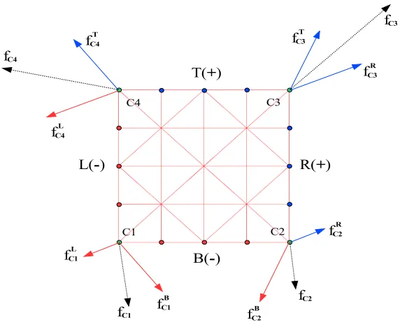
7.5. Antiperiodicity of forces at the corners

The antiperiodicity is represented by means of forces at the corners as depicted in Figure 4. The superscripts indicate the following:

B Bottom (₋)

T Top (+)

L Left (₋)

R Right (+)

Figure 4: Discrete forces at the corners

The forces at the corners represent the discretization of the traction coming from the surrounding continuum.

• Corner 1 (C1): f_c1B and f_c1L

• Corner 2 (C2): fB

c2 and fc2R • Corner 3 (C3): f_c3R and f_c3T

There are two forces per corner making a total of 8 at the discretised RVE. These forces must satisfy antiperiodicity. Therefore, the following 4 equations for antiperiodicity at the corners are established as,

f_c1B=₋f_c4T f_c2B=₋f_c3T fL

c1=−fc2R

f_c4L =₋f_c3R

(75)

The resultant at each corner is also described on the Figure 4. Four additional relations are obtained as follows,

f_c1B+f_c1L =fc1

f_c2B+f_c2R =fc2

fR

c3+fc3T =fc3

f_c4L +f_c4T =fc4

(76)

Then, the system formed by the equations (75) and (76) is reduced to have only one force per corner. This leads to,

fc1+fc2+fc3+fc4=0 (77)

Equation (77) is the additional condition to apply to the system in order to compute the tangent operator. (77) expresses the continuum antiperiodicity traction constraint and makes the system to be in equilibrium.

7.6. Condensation of the d.o.f. corresponding to fc1

The equilibrium and antiperiodicity equation at the corners of the discretised RVE is given by (77) which is imposed to compute the overall tangent modulus. The first two rows of KC1 and

KC2 (corresponding to the 2 dofs offc1) have to be removed and recomputed by adding the other 6 rows (2 by 2) and, then, multiplied by -1. This process is visually described in Figure 5.

7.7. Microequilibrium computation for periodic b.c.

In Section 4 a general solution scheme for microequilibrium was given. In this section, the particularisation of the microequilibrium procedure for periodic b.c. is given. The incremental Taylor displacement is given in matrix form as,

△u∗

=DT_{global,p△ǫ (78)}

Figure 5: Elimination and recalculation fromKC1andKC2toKˆC1andKˆC2

r=

f_iint f_pint+f_nint

−

f_iext f_pext+f_next

(79)

Assuming that in equilibriumfext

i =0and antiperiodicity of the boundary traction in discrete form

f_pext+f_next=0, the residual for periodic b.c. takes the form,

r=

f_iint fint

p +fnint

. (80)

The differential fluctuation is given by the system (12) which takes the following form for periodic b.c.

K2

δuei

δ_eup

=₋

f_iint f_pint+f_nint

→

δeui

δu_ep

=₋K−₁ 2

f_iint f_pint+f_nint

(81)

for differential displacement fluctuation for interior and positive nodes. Also taking into consider-ation (46) and (44), the differential displacement fluctuconsider-ation for negative and corners is computed as,

δuen=δuep and δuec=0 (82)

The updating of the incremental fluctuation is then given by

△uei ← △uei+δeui △eup ← △eup+δeup △eun ← △eup

(83)

△ui ← △ui+δeui △up ← △up+δeup △un ← △up

(84)

and _△uc remains constant.

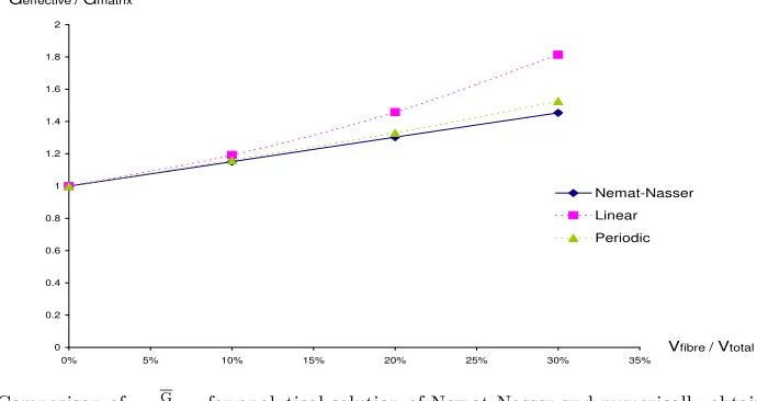
8. Computation of elastic properties for a composite at small strain

The first numerical test consists of computation of effective elastic material properties. Square microcells, in which fibres are periodically distributed, are considered composed of epoxy matrix with Young’s modulusE= 3.13 GP a and Poisson’s ratioν = 0.34. Glass fibre is embedded in the matrix with Young’s modulusE = 73GP a and Poisson’s ratio ν= 0.2.

The test has been carried out under plane strain analysis. In Figure 6 the ratio of effective shear modulus over the matrix modulus G/Gmatrix is compared with analytically obtained properties

following Nemat-Nasser (Part I, chapter 8) [29].

A very similar response can be observed for less than 20% of the inclusion volume fraction. Especially, the periodic assumption seems to be very accurate. Note that the Nemat-Nasser’s analytical model is effective in predicting equivalent material properties for a low volume fraction of the second phase inclusion. However, Nemat-Nasser’s model [29] does not cope well with large fibre volumes.

0 0.2 0.4 0.6 0.8 1 1.2 1.4 1.6 1.8 2

0% 5% 10% 15% 20% 25% 30% 35%

Vfibre / Vtotal Geffective/ Gmatrix

Nemat-Nasser Linear Periodic

Figure 6: Comparison of G

Gmatrix for analytical solution of Nemat-Nasser and numerically obtained results.

9. Internally pressurised elasto–plastic circular plate at small strain

plate, see Figure 7. The analysis is carried out assuming plane stress conditions. Note that the equality between the macroscopic strain and the average of the microscopic strain -imposed as an average on the RVE- is satisfied by means of application of the Hill-Mandel principle or averaging theorem. The von Mises perfect elastoplastic model is used to perform the simulation.

The properties of the material are as follows:

• Young’s modulus E = 210 GPa. • Poisson ratioν = 0.3.

• uniaxial yield stress σy = 0.24 GPa (perfect elastoplastic).

Figure 7: Internally pressurised circular plate. Quarter of circular plate mesh

The mesh for the macrostructure is shown in Figure 7. Due to symmetry only a quarter of the circular plate is analyzed by employing 20 standard 8-noded quadrilateral elements with reduced integration.

begins. In this region the radial displacement of the outer surface is a linear function ofP, given by:

ub =

2P b E(_ab22 −1)

P < P0 (85)

A closed-form in the plastic region, has been derived by Lubliner [30]. It relates the applied pressure to the radiusc of the plastic front by means of the expression:

P Y = ln

c a

+1 2

1₋c 2

b2

, (86)

where, for the von Mises modelY = 2σy/

√

3. Plastic yielding begins whenc=a, which corresponds to the yielding pressure:

P0

Y =

1 2

1₋a 2

b2

. (87)

In the plastic regime (P _≥P0 ), the radial displacement,ub, is given by

ub = Y c2

Eb P < P0 (88)

wherec can be evaluated as an implicit function of P through (86).

9.1. Internal pressure vs outer surface displacement diagrams

In the following figures, diagrams showing the applied pressure P versus radial displacement at the outer face of the plate are plotted together with the closed-form solution [30] described above. The following diagrams are displayed:

• Single scale analysis: Closed form and FEM analysis

• Two multi-scale analyses. RVE: Square microstructure discretized by 8-noded quadrilateral elements with reduced integration. Every cell has a void in the middle with variable shape and volume fraction, as follows:

– Microstructure 1: Circular void in the middle of the RVE with 5 % volume fraction. nelements= 126 , nnodes= 438.

– Microstructure 2: Square void in the middle of the RVE with 5 % volume fraction. nelements= 128 , nnodes= 448.

nelements= 128 , nnodes= 448.

– Microstructure 3: Circular void in the middle of the RVE with 15 % volume fraction. nelements= 128 , nnodes= 448.

– Microstructure 4: Square void in the middle of the RVE with 15 % volume fraction. nelements= 160 , nnodes= 560.

These microstructures are depicted in Figure 9.

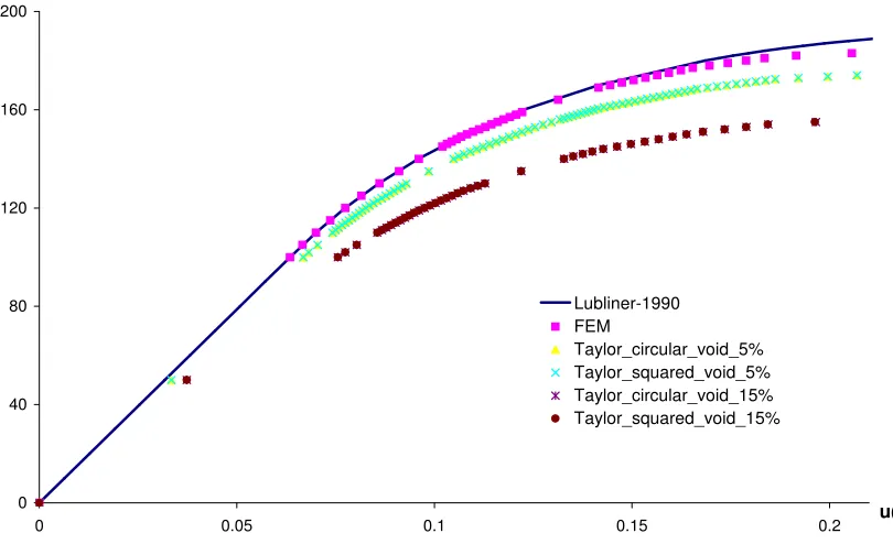
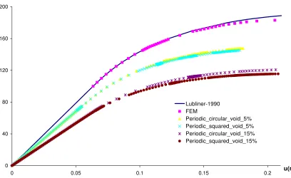
In Figures 10, 11 and 12 results are shown for different constraints on the microcell and 5 and 15% void fraction, respectively. Curved denoted Lubliner-1990 represents the closed-form solution described above and given in [30]. FEM curve shows a single scale analysis of the problem. The agrement between the closed form and FEM solution is excellent. Furthermore, two scales analysis curves are depicted for Taylor assumption, linear b.c and periodic b.c. The comments are as follows:

• Taylor assumption gives the stiffest response. Then comes linear b.c. while the softest response is given by periodic b.c. This was expected from the nature of the constraints. • Taylor assumption and linear b.c. show insensitivity at macroscopic level for different void

shape. Diagrams for circular and squared void shape are overlapped.

• Periodic b.c. is the only one which shows sensitivity to the void size. It can be observed that circular void gives slightly stiffer response than the square one, which agrees with the expected response. Moreover, the difference is bigger when the void size is increased.

Figure 9: Microstructures for analysis of internally pressurised circular plate

0 40 80 120 160 200

0 0.05 0.1 0.15 0.2 u(mm)

P(MPa)

Lubliner-1990 FEM

Taylor_circular_void_5% Taylor_squared_void_5% Taylor_circular_void_15% Taylor_squared_void_15%

0 40 80 120 160 200

0 0.05 0.1 0.15 0.2 u(mm)

P(MPa)

Lubliner-1990 FEM

Linear_circular_void_5% Linear_squared_void_5% Linear_circular_void_15% Linear_squared_void_15%

Figure 11: Internally pressurised circular plate. Pressure vs displacement (ub) diagram for the linear b.c.

0 40 80 120 160 200

0 0.05 0.1 0.15 0.2 u(mm)

P(MPa)

Lubliner-1990 FEM

Periodic_circular_void_5% Periodic_squared_void_5% Periodic_circular_void_15% Periodic_squared_void_15%

Figure 12: Internally pressurised circular plate. Pressure vs displacement (ub) diagram for the periodic b.c.

9.2. Effective Plastic Strain Distribution

a circular way which agrees with the symmetry of the problem and the analytical solution given earlier [30].

In Figure 13 a Microstructure 1 is considered under the Taylor assumption. Two different stages are depicted at different values of internal pressureP = 140 and P = 175MPa, respectively. The circular evolution of the plastic front at macroscale level can be observed. ForP = 175MPa a slight distortion of the plastic front is visible as the load approaches the limit value.

In Figures 14(a) and 14(b) the results for the linear b.c. are shown for Microstructure 1 for values of internal pressure ofP = 100 andP = 160MPa, respectively, while Figures 15(a) and 15(b) give the result for the periodic b.c. for values of internal pressure of P = 95 and P = 150MPa, respectively. The development of shear bands is observed in these figures.

Figure 13: Effective plastic strain for the Taylor assumption. Microstructure: circular void at 5% volume fraction

(a)P _{= 100 MPa (b)}P _{= 160 MPa}

(a)P _{= 95 MPa (b)}P _{= 150 MPa}

Figure 15: Effective plastic strain distribution for the periodic b.c. Microstructure 1: circular void at 5% volume fraction

In Figure 16 the Microstructure 2 is considered under the Taylor assumption. Again two different stages are depicted for different values of internal pressureP = 140 andP = 175MPa, respectively. For P = 175MPa a slight distortion of the plastic front is visible as the load approaches the limit value.

In Figures 17(a) and 17(b) the results for the linear b.c. are shown for Microstructure 2 for values of internal pressure ofP = 100 andP = 160MPa, respectively, while Figures 18(a) and 18(b) give the result for the periodic b.c. for values of internal pressure of P = 95 and P = 150MPa, respectively. The development of shear bands is observed in these figures.

Figure 16: Effective plastic strain for the Taylor assumption. Microstructure: squared void at 5% volume fraction

(a)P _{= 100 MPa (b)}P _{= 160 MPa}

Figure 17: Effective plastic strain distribution for the linear b.c. Microstructure 2: square void at 5% volume fraction

stages are depicted for different values of internal pressureP = 115 andP = 160MPa, respectively. The circular evolution of the plastic front at macroscale level is shown. Again, for P = 160MPa a slight distortion of the plastic front is visible as the load approaches to the limit value.

In Figures 20(a) and 20(b) the results for the linear b.c. are shown for Microstructure 3 for values of internal pressure ofP = 100 andP = 130MPa, respectively, while Figures 21(a) and 21(b) give the result for the periodic b.c. for values of internal pressure of P = 100 andP = 120MPa, respectively. The development of shear bands is observed in these figures.

In Figure 22 a Microstructure 4 is considered under the Taylor assumption. Two different stages are depicted for different values of internal pressure P = 115 and P = 160MPa, respectively. For

P = 160MPa a slight distortion of the plastic front is visible as the load approaches the limit value. In Figures 23(a) and 23(b) the results for the linear b.c. are shown for Microstructure 1 for values of internal pressure ofP = 90 andP = 130MPa, respectively, while Figures 24(a) and 24(b) give the result for the periodic b.c. for values of internal pressure of P = 75 and P = 115MPa, respectively. The development of shear bands is observed in these figures.

9.3. Residuals evolution per iteration in macro and micro levels

In this section tables with the Euclidean norm RM of the residual are reported associated with the Newton iterations of the macro- and micro-equilibrium. The residual norm evolution is shown for the microstructure that corresponds to the macro Gauss point in the bottom right corner.

In the following tables the Euclidean norm RM of the residual is reported associated with the Newton iterations of the macro-equilibrium. The macro-residual is normalised and calculated as RM = 100× kFint−Fextk/kFextk. The micro residual is computed in different ways depending

(a)P _{= 75 MPa (b)}P _{= 145 MPa}

Figure 18: Effective plastic strain distribution for the periodic b.c. Microstructure 2: square void at 5% volume fraction

Figure 19: Effective plastic strain for the Taylor assumption. Microstructure: circular void at 15% volume fraction

The residual for linear b.c. is evaluated as Rµ= 100× krk/kfintk wherer is given asr=fiint. The residual for periodic b.c. is evaluated as Rµ= 100× krk/kfintk whererwas given in (80).

Clearly, the quadratic rate of asymptotic convergence can be observed in the macro and microscale for both Linear and Periodic b.c.’s. Also the Taylor assumption shows quatratic rate of convergence in macroequilibrium.

(a)P _{= 100 MPa (b)}P _{= 130 MPa}

Figure 20: Effective plastic strain distribution for the linear b.c. Microstructure 3: circular void at 15% volume fraction

Macro-step RM

1 2.049263×10−02

2 1.340442×₁₀−06

3 1.676496×₁₀−13

Table 1: Evolution of Residual norm at the Macroscale (RM) for Taylor constraint assuming Microstructure 3 (15% circular void). Increment of internal pressure P = 115-116 MPa

In Taylor it is more obvious since it is presented at larger pressure.

10. Conclusion

(a)P _{= 100 MPa (b)}P _{= 120 MPa}

Figure 21: Effective plastic strain distribution for the periodic b.c. Microstructure 3: circular void at 15% volume fraction

(a)P _{= 90 MPa (b)}P _{= 130 MPa}

Figure 23: Effective plastic strain distribution for the linear b.c. Microstructure 4: square void at 15% volume fraction

(a)P _{= 75 MPa (b)}P _{= 115 MPa}

micro Rµ Macro RM 1 2.947000×₁₀−00

2 7.483573×10−01

3 4.572174×₁₀−02

4 1.965543×10−04

5 1.635712×₁₀−09 1 _3.569328×₁₀−02 1 2.985146×10−00

2 1.255292×₁₀−00

3 8.916588×₁₀−02

4 6.666795×10−04

5 7.972844×₁₀−09 _{2 4.463401}×₁₀−06

1 2.985146×₁₀−00

2 1.255292×₁₀−00

3 8.916583×10−02 4 6.666805×₁₀−04

5 7.972878×₁₀−09 _{3 4.152282}×₁₀−12

micro Rµ Macro RM

1 7.570612×₁₀−00

2 2.273063×₁₀+01 3 1.220398×10−00 4 1.857460×₁₀−01

5 4.258028×₁₀−03

6 9.028518×10−07

7 5.974417×₁₀−12 1 _6.801729×₁₀−02

1 7.685538×₁₀−00

2 2.287550×₁₀+01 3 1.240264×10−00 4 1.914852×₁₀−01

5 1.531063×₁₀−02

6 3.075176×10−06

7 1.719892×₁₀−11 2 _6.902391×₁₀−04

1 7.685065×₁₀−00 2 2.287559×₁₀+01 3 1.240250×10−00 4 1.914694×₁₀−01 5 1.530919×₁₀−02

6 3.074341×₁₀−06

7 1.719583×10−11 3 3.157912×10−09 1 7.685065×10−00

2 2.287559×₁₀+01 3 1.240250×₁₀−00

4 1.914694×10−01 5 1.530919×₁₀−02

6 3.074341×₁₀−06

7 1.718875×10−11 4 1.687747×10−13

a Linear b.c. b Periodic b.c.

Table 2: Evolution of Residual norm at micro (Rµ) and Macroscale (RM) for Linear b.c. and Periodicb.c. assuming

References

[1] Eshelby J.D. The determination of the field of an ellipsoidal inclusion and related problems. Proceeding of the Royal Society of London, 241:376–396, 1957.

[2] Hashin Z. The elastic moduli of heterogeneous materials. Journal of Applied Mechanics, 29:143–150, 1962.

[3] Mori T. and Tanaka K. Average stress in the matrix and average elastic energy of materials with misfitting inclusions. Acta Metallurgica, 21:571–574, 1973.

[4] Nan C.W. and Clarke D.R. The influence of particle size and particle fracture o the elas-tic/plastic deformation of metal matrix composite. Acta Materialia, 44(9):3801–3811, 1996. [5] Hashin Z. Analysis of composite materials. a survey.Journal of Applied Mechanics, 50:441–505,

1983.

[6] Ponte Casta neda P. and Suquet P. Nonlinear composites. Advances in Applied Mechanics, 34:171–302, 1998.

[7] Bensoussan A. Lions J.L. and Papanicolaou G. Asymptotic analysis for periodic strucutres, in: Studies in Mathematics and its Applications. North Holland Publishing Company, 1978. [8] E. Sanchez-Palencia. Non-homogeneous media and vibration theory. Lecture notes in physics.

Number 127. Springer-Verlag, Berlin, 1980.

[9] Torquato S. Random Heterogeneous Materials. Microestructure and Macroscopic Properties. 2002.

[10] Toledano A. and Murakami H. A high-order mixture model for periodic particulate composites. International Journal of Solids and Structures, 23:989–1002, 1987.

[11] Guedes J.M. and Kikuchi N. Preprocessing and postprocesing for materials based on the homogenization method with adaptative finite element methods.Computer Methods in Applied Mechanics and Engineering, 83:143–198, 1990.

[12] Fish J. Shek K. Pandheeradi M. and Shephard M.S. Computational plasticity for composite structures based on mathematical homogenization: Theory and practice. Computer Methods in Applied Mechanics and Engineering, 148:53–73, 1997.

[13] Chung P.W. Tamma K.K. and Nambutu R.R. Asymptotic expansion homogenization for heterogeneous media: computational issues and applications. Composites. Part A: applied science and manufacturing, 32:1291–1301, 2001.

[14] Christman T. Needleman A. and Suresh S. An experimental and numerical study of deforma-tion in metal-ceramic material. Acta Metallurgica, 37(11):3029–3050, 1989.

[16] Nakamura T. and Suresh S. Effect of thermal stress and fiber packing on deformation of metal-matrix composite. Acta Metallurgica et Materialia, 41(6):1665–1681, 1993.

[17] van der Sluis O. Schreurs P.J.G. and Meijer H.E.H. Effective properties of viscosplastic con-stitutive model obtained by homogenization. Mechanics of Materials, 31:743–759, 1999. [18] Ohno N. Wu X. and Matsuda T. Homogenized properties of elastic-viscoplastic composites

with periodic internal structures. International Journal of Mechanical Science, 42:1519–1536, 2000.

[19] Swan C.C. Techniques for stress- and strain-controlled homogenization of inelastic periodic composites. Computer Methods in Applied Mechanics and Engineering, 117:249–267, 1994. [20] Swan C.C. and Cakmak A.S. Homogenization and elastoplasticity models for periodic

com-posites. Communication in Numerical Methods and Engineering, 10:257–265, 1994.

[21] Swan C.C. and Kosaka I. Homogenization-based analysis and design of composites. Computer and Structures, 64:603–621, 1997.

[22] Suquet P.M. Local and global aspects in the mathematical theory of plasticity, pages 279–310. In Sawczuk A. and Bianchi G. editors, Plasticity today: modelling, methods and applications. London. Elsevier Applied Science Publishers, 1985.

[23] Terada K. and Kikuchi N. Computational Methods in Micromechanics, volume 212, chapter Nonlinear homogenization method for practical application, pages 1–16. ASME, 1995.

[24] Ghosh S. Lee K. and Moorthy S. Multiple scale analisys of heterogeneous elastic structures using homogenization theory and voroni cell finite element method. International Journal of Solids and Structures, 32(1):27–62, 1995.

[25] Zohdi T.I. Oden J.T. Rodin G.J. Hierarchical modelling of heterogeneous bodies. Computer Methods in Applied Mechanics and Engineering, 138:273–298, 1996.

[26] Miehe C. Schotte J. and Schroder J. Computational micro-macro transitions and overall tangent moduli in the analysis of polycrystals at large strains.Computational Material Science, 16:372–382, 1999.

[27] Miehe C. Schroder J. and Schotte J. Computational homogenization analysis in finite plasticity. simulation of texture development in polycrystalline materials. Computer Methods in Applied Mechanics and Engineering, 171:387–418, 1999.

[28] Matsui K. Terada K. and Yuge K. Two-scale finite element analysis of heterogeneous solids with periodic microstructures. Computers and Structures, 82:593–606, 2004.

[29] Nemat-Nasser S. and Hori M. Micromechanics: overall properties of heterogeneous materials. Elsevier, 1999. Part I, chapter 8.