Using Existing Stated Preference Data to Analyse Bus Preferences

This is a repository copy of

Using Existing Stated Preference Data to Analyse Bus

Preferences

.

White Rose Research Online URL for this paper:

http://eprints.whiterose.ac.uk/2070/

Monograph:

Wardman, M. (2000) Using Existing Stated Preference Data to Analyse Bus Preferences.

Working Paper. Institute of Transport Studies, University of Leeds , Leeds, UK.

Working Paper 555

[email protected] https://eprints.whiterose.ac.uk/ Reuse

See Attached

Takedown

If you consider content in White Rose Research Online to be in breach of UK law, please notify us by

White Rose Research Online

http://eprints.whiterose.ac.uk/

Institute of Transport Studies

University of Leeds

This is an ITS Working Paper produced and published by the University of

Leeds. ITS Working Papers are intended to provide information and encourage

discussion on a topic in advance of formal publication. They represent only the

views of the authors, and do not necessarily reflect the views or approval of the

sponsors.

White Rose Repository URL for this paper:

http://eprints.whiterose.ac.uk/

2070/

Published paper

Mark Wardman (2000)

Using Existing Stated Preference Data to Analyse Bus

Preferences.

Institute of Transport Studies, University of Leeds, Working Paper

555

September

2000

USING EXISTING STATED PREFERENCE DATA

TO ANALYSE BUS PREFERENCES

Mark Wardman

ITS Working Papers are intended to p ovide information and encourage discussion

on a topic in advance of formal publication. They represent only the views of the

authors, and do not necessarily reflect the views or approval of the sponsors.

.

September 2000

Using Existing Stated Preference Data to

Analyse Bus Preferences

INSTITUTE FOR TRANSPORT STUDIES

DOCUMENT CONTROL INFORMATION

Title

Using Existing Stated Preference Data to Analyse Bus

Preferences

Author(s) Mark

Wardman

Editor

Reference Number

WP555

Version Number

1.0

Date September

2000

Distribution Public

Availability unrestricted

File K\office\workpaps\wp555

Authorised O.M.J.

Carsten

Signature

CONTENTS

1.

INTRODUCTION AND OBJECTIVES ...2

2.

BACKGROUND ...3

3.

THE PREVIOUS STUDIES...3

3.1

Clitheroe Rail Study...4

3.2

Nottingham-Mansfield Rail Study...4

3.3

Nottingham LRT Study...4

3.4

Summary of Studies...5

4.

INITIAL BUS-TRAIN MODEL ...5

5.

ANALYSIS OF VARIATIONS IN BUS USERS’ COST COEFFICIENTS ...7

5.1

Factors of Interest ...7

5.2

Impact of Current Fare Level and Direction and Magnitude of Fare Change ...7

5.3

Impact of Level of Service...8

5.4

Impact of Socio-Economic Variables ...9

5.5

Final Bus-Train Mode Choice Model ...10

6.

THE STATED PREFERENCE EVIDENCE AND ELASTICITY VARIATION ...11

6.1

Variations in Sensitivity to Cost ...11

6.2

Comparison of SP Results with Findings of the Aggregate Econometric Study...12

6.2.1

Results at a National and Regional Level ...13

6.2.2

Results at a County Level ...14

7.

CONCLUDING REMARKS...16

References...17

APPENDIX 1: CLITHEROE RAIL STUDY SP DESIGNS ...19

APPENDIX 2: NOTTINGHAM-MANSFIELD STUDY SP DESIGNS...20

APPENDIX 3: NOTTINGHAM LRT STUDY SP DESIGN...21

USING EXISTING STATED PREFERENCE DATA

TO ANALYSE BUS PREFERENCES

1.

INTRODUCTION AND OBJECTIVES

The purpose of this research is to re-analyse existing Stated Preference (SP) data sets which provide information on preferences towards bus in order to complement analysis commissioned by DETR which is concerned with bus fare elasticities and which is conducted at a much more aggregated level.

The data sets available relate solely to urban/suburban travel and to studies for which ITS had prime responsibility. The objectives of this re-analysis of previous bus users' SP data sets were to address the following issues:

• How the sensitivity to cost varies with income, age and gender in addition to journey purpose. Analysis of the effect of income on the cost coefficient is essentially the same as analysis of how the value of time varies with income.

• Whether there is a non-linear relationship between the sensitivity to fare and the level of fare.

• Whether the sensitivity to fare varies according to whether the fare level in the SP exercise implied an increase or reduction on current levels. This would follow along the lines of similar analysis conducted on the sensitivity to time losses and gains in several recent value of time studies.

• How the magnitude of the fare change impacts upon the sensitivity to cost. This can be examined given that we are in a position to deduce whether the SP exercise implied an increase or reduction in the fare.

• Whether the quality of service offered influences the sensitivity to cost variations; for example, bus users may be less sensitive to cost increases where the service quality is good.

2. BACKGROUND

This research was intended to complement analysis using aggregate data commissioned by DETR (Dargay and Hanly, 1999). The latter provides aggregate bus fare elasticities and is well suited to the analysis of specific issues, such as lagged behavioural response, but only limited segmentation of the elasticities, such as by region, is possible. Whilst in principle the analysis could examine whether the bus fare elasticity is different for fare increases and reductions and also according to the size of the fare change, in practice such analysis is hampered because of data limitations.

This approach can be supplemented by analysis based on disaggregate methods.

SP methods avoid such data limitations, such as lack of variation and collinearity, and can provide more detailed segmentations. They support detailed analysis regarding the sensitivity to bus fare changes as well as changes to bus service quality attributes. Rather than conducting fresh survey work, it is sensible to determine whether existing SP data sets can be exploited to provide insights into relevant issues.

The opportunity exists to re-analyse SP data since, in the vast majority of previous studies, relatively simple SP choice models were developed which satisfied the immediate forecasting needs of the project in question. In general, there has been a tendency for journey purpose to be the only socio-economic variable which was used to segment SP choice models. In any event, there was little point examining how the sensitivity to cost varies with, say, income group if the origin-destination matrix could not be segmented by income. Moreover, the simplest possible form of utility expression was typically specified which implies that:

• the sensitivity to changes in some bus attribute is the same regardless of the level of the attribute, and the size and direction of the change in the attribute.

• the sensitivity to changes in some bus attribute is not allowed to interact with the level of other bus attributes.

• the sensitivity to changes in some bus attribute is constrained to be the same as the sensitivity to changes in the equivalent attribute for some other mode.

Hence standard mode choice models developed in Great Britain tend to provide little indication as to whether the bus fare elasticity is conditioned by the level of fare itself or the level of service quality offered, or how it varies with little other than journey purpose. However, existing SP data sets allow such analysis to be undertaken. Two comprehensive reviews of the use of mode choice models in Great Britain are provided by Wardman (1997a) for urban travel and Wardman (1997b) for inter-urban travel.

3.

THE PREVIOUS STUDIES

3.1

Clitheroe Rail Study

The bus users in the Clitheroe rail study were offered two SP exercises, each involving 9 pairwise comparisons of bus and rail. One SP exercise contained fare, in-vehicle time and out-of-vehicle time for train and bus, with headway specified to be constant for both train and bus at an hourly frequency. The other SP exercise varied fare, in-vehicle time and frequency for bus and train and specified out-of-vehicle time to be ‘as now’. The actual SP designs used are listed in Appendix 1.

A self completion exercise was used and the sample contained 50 individuals reflecting a response rate of 51%. The data was collected in 1990 and the segmentation variables available are age, gender, income and journey purpose. Further details about this study are contained in the final report (Preston, 1991). For the bus-train model, the key findings were that travel time, including out-of-vehicle time, was valued at 2.25 pence per minute, with no distinction between train and bus. The mode constant favoured train by 23 pence for non-commuting trips but favoured bus by 10 pence for commuting and education trips. The bus service interval was valued at 0.55 pence per minute but no significant effect was discerned for train frequency.

3.2 Nottingham-Mansfield

Rail

Study

The bus users in the Nottingham-Mansfield rail study were also offered two SP exercises, each involving 9 pairwise comparisons of bus and rail. One SP exercise contained fare, in-vehicle time and out-of-vehicle time for train and bus, with headway for bus specified to be as now and train headway held constant at an hourly frequency. The other SP exercise varied fare and in-vehicle time for bus and train and also train frequency, with bus frequency and out-of-vehicle time for bus and train specified to be ‘as now’.

Separate SP exercises were offered according to distance from Nottingham. The actual SP designs used are listed in Appendix 2.

A self completion exercise was used and the sample contained 577 individuals with a 50% response rate overall. The data was collected in 1988 and the segmentation variables available are age, gender, income and journey purpose.

Further details about this study are contained in the final report (Preston and Wardman, 1989a). Separate models were estimated for the longer distance trips originating in the Mansfield area and the shorter distance trips from the outskirts of Nottingham. Neither model distinguished the coefficients by mode. The values of time for the longer and shorter distance trips were 1.6 and 0.9 pence per minute, with out-of-vehicle time values of 2.2 and 1.1 pence per minute respectively. The constant favoured train to the extent of 8.9 and 2.3 pence for the longer and shorter distance trips respectively, but service frequency was only estimated to have a significant influence on choices for the shorter distance trips. No segmentation by journey purpose was reported.

3.3

Nottingham LRT Study

The bus users in the Nottingham LRT study were offered 16 pairwise comparisons of bus and LRT. Each mode was described in terms fare, in-vehicle time, out-of-vehicle time and frequency. The actual SP design used is listed in Appendix 3.

A self completion exercise was used and the sample contained 180 individuals who were all commuters. The response rate amongst bus users was 32%. The data was collected in 1989 and the segmentation variables available are age, gender and income.

constant was found to favour LRT to the extent of 8 pence with estimated values of walking and in-vehicle time of 2.3 and 0.8 pence per minute. The value of an additional bus or LRT service per hour was estimated at 0.9 pence.

3.4

Summary of Studies

The same basic approach of self completion questionnaire was administered in each of the three studies, with the same variables used in each SP experiment. In each case, an initial travel behaviour questionnaire had been completed and had recruited those who were willing to participate further in the study by answering the SP questionnaire.

In all three of the studies, models were estimated with correct sign and statistically significant coefficients and reasonable goodness of fit measures were achieved. The values of time, in the prices then applying, were generally reasonable. However, no allowances were made for mode-specific valuations of the attributes and the models were specified such that the sensitivity to any particular attribute was constant regardless of its level or whether it represented an increase or reduction on the individual’s current position.

4.

INITIAL BUS-TRAIN MODEL

In this re-analysis of the three existing data sets relating to the choices made between train and bus by current bus users, we make maximum use of the available data by estimating a single model to the pooled data sets. This is justified on the grounds of the reasonably similar results obtained by each study, although we did allow for differences across the data sets by specifying site specific dummy variables. In addition, and in the light of the somewhat different cost and time levels used in each SP experiment, we have also experimented with the use of variables specified per unit of distance. This will have no impact on whether the fare change is specified to be an increase or a reduction, nor on whether the change is ‘large’ or ‘small’, but it is relevant to the analysis of the effect of fare level on the sensitivity to fare changes and whether sensitivity is influenced by the absolute fare or fare per mile. It is then an empirical issue as to whether the model which specifies variables deflated by distance provides a better explanation of choices than one which does not.

The bus-train mode choice model combines the SP data obtained from three separate studies. After removing records where no SP response was supplied, or where there was indifference between the two modes, yields the following number of observations for each data set:

• Blackburn-Clitheroe Rail Study: 850 observations • Nottingham-Mansfield Rail Study: 7110 observations • Nottingham LRT Study: 2816 observations

Of the total number of 10776 SP choices, 4480 were for bus and 6296 were for train. In each study, the attributes used to characterise bus and train were cost, in-vehicle time (IVT), out-of-vehicle time (OVT) and headway.

Initial models for the combined data set are reported in Table 4.1, expressed in one-way units of pence and minutes, with one model ‘normalising’ the cost variables by deflating by distance and the other using the conventional absolute specification. The initial utility function for each mode i is therefore:

i i i i i i i i i

i

C

T

O

H

U

=

α

+

λ

+

µ

+

φ

+

η

The model which entered cost and IVT without any distance adjustment, and reported in the final column of Table 4.1, obtained a ρ2 goodness of fit of 0.208. This increased to 0.214 when the costs were deflated by distance and which is the other model reported. In our experience, this is a large improvement in fit after changing the specification of only two variables. However, additionally deflating IVT by distance reduced ρ2 to 0.194 and hence normalisation has been restricted to the cost terms. This model specification is, we believe, quite novel since we are unaware of studies that have examined choices based on cost per mile.

[image:11.595.76.334.250.399.2]

Not only have we obtained models which have a goodness of fit far higher than is typically obtained in SP mode choice models, the models have number of other desirable properties.

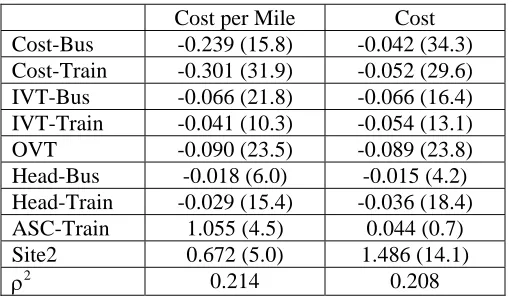
Table 4.1: Overall Bus-Train Mode Choice Model

Cost per Mile Cost

Cost-Bus -0.239 (15.8) -0.042 (34.3)

Cost-Train -0.301 (31.9) -0.052 (29.6)

IVT-Bus -0.066 (21.8) -0.066 (16.4)

IVT-Train -0.041 (10.3) -0.054 (13.1)

OVT -0.090 (23.5) -0.089 (23.8)

Head-Bus -0.018 (6.0) -0.015 (4.2)

Head-Train -0.029 (15.4) -0.036 (18.4)

ASC-Train 1.055 (4.5) 0.044 (0.7)

Site2 0.672 (5.0) 1.486 (14.1)

ρ2 _{0.214 0.208}

All the coefficients are of the correct sign and are highly statistically significant. We allowed the coefficients to vary by mode and, with the exception of OVT which had very similar coefficients by mode, this has been justified. It is important to allow the cost coefficients to vary by mode since, in this study, we are particularly interested in the response of current bus users to bus cost, whilst there are reasons for expecting other coefficients to differ between train and bus.

In both models, the cost coefficient is higher for train than bus, and this may well stem from the higher fares associated with rail than bus. That the cost coefficient is larger for train than bus is encouraging with regard to the quality of the SP responses provided since, given the sample is entirely made up of bus users, any protest responses or strategic response bias would be expected to lead to a larger coefficient for bus cost than train cost other things equal.

The OVT coefficient is higher than the IVT coefficients, as expected, whilst the headway coefficient is larger for train than bus which may well stem from the generally larger headways between trains than buses in the SP exercises. We might expect the disutility of time spent on a bus to exceed that of time spent on a train, and the IVT coefficients indicate that this is indeed the case although the effect is not particularly large. The constant is consistent with our prior expectations in that it favours train, with an additional effect for bus users in the Nottingham-Mansfield (Site2) sample.

The estimated value of time in the distance normalised model will not only vary according to mode but it will also depend on distance given the specification of the cost variables. Indeed, the value of time will increase with distance, an effect which was apparent in a recent review of values of time (Wardman, 1999).

GDP elasticity of one, these values become 3.96, 5.41 and 1.96 respectively. These values seem entirely plausible. Another reason for preferring the normalised model is that the values of IVT and OVT for bus in the non-normalised model are 1.57 and 2.11, which in current prices are 2.65 and 3.56 respectively, and these seem less plausible.

The estimated model therefore provides a firm basis upon which to conduct our analysis of the sensitivity of different types of bus users to cost variations. We prefer the normalised model but we continue to report the findings of the non-normalised model in our subsequent discussions.

5.

ANALYSIS OF VARIATIONS IN BUS USERS’ COST COEFFICIENTS

5.1

Factors of Interest

As outlined in the introduction, and following the objectives set out in the proposal, the re-analysis of the bus users’ SP data examines the following issues:

• How the sensitivity to cost varies with income, age, gender and journey purpose.

• Whether there is a non-linear relationship between the sensitivity to fare and the level of fare

• Whether the fare level in the SP exercise implied an increase or reduction on current levels and its impact on choices

• Whether the magnitude of the change in fare in the SP exercise influences bus users’ sensitivity to it.

• Whether the quality of service offered influences the sensitivity to cost variations.

5.2

Impact of Current Fare Level and Direction and Magnitude of Fare Change

We amended the utility function as it relates to the bus fare to allow the sensitivity to cost changes to vary with the current fare and both the direction and size of the fare change in the SP exercise. The utility function with respect to the cost of bus (either per mile or in absolute) which is denoted C was specified as:

...

)

(

)

(

3 2 2 2 2 1

1

−

+

−

+

+

+

+

=

C

CF

d

C

F

d

C

F

d

C

U

α

β

γ

γ

δ

where F is the fare level (either per mile or in absolute) currently faced by the respondent, d1 and d2

denote respectively whether the SP cost is an increase or reduction on the current fare, and d3 is a

dummy variable denoting whether the base fare was zero.

The sensitivity to cost variations, represented by the marginal utility of cost, in this utility expression is: ... ) ( 2 ) (

2 _{1 1} − + _{2 2} − + ₃ +

+ + = ∂ ∂ d F C d F C d F C

U

_α

_β

_γ

_γ

_δ

The conventional model is obtained if β, γ1, γ2 and δ are each insignificantly different from zero. The

[image:13.595.76.525.96.167.2]

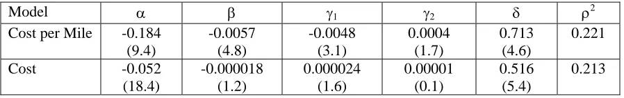
Table 5.1: Model of Effects of Fare Level and Sign and Size of Fare Change

Model α β γ1 γ2 δ ρ2

Cost per Mile -0.184 (9.4) -0.0057 (4.8) -0.0048 (3.1) 0.0004 (1.7) 0.713 (4.6) 0.221 Cost -0.052 (18.4) -0.000018 (1.2) 0.000024 (1.6) 0.00001 (0.1) 0.516 (5.4) 0.213

With regard to the normalised model, it can be seen that all but one of the parameters of the estimated model is statistically significant with the remaining estimate not being far from significant. The sensitivity to cost changes is higher at higher levels of current fare (β), which is consistent with diminishing marginal utility of income.

The sensitivity to cost changes is higher for larger cost (γ1) increases and for larger cost reductions

(γ2). In the latter case, γ2 is positive but the C-F term is negative. However, the size of cost reductions

has only a very minor impact on the sensitivity to cost changes. However, we must remember that we only have bus users in the sample and hence bus fare reductions might be expected to have less impact on behaviour than increases. Nonetheless, it would be interesting to examine whether this effect was also apparent for non-users.

Those with zero fares have a low sensitivity to fare changes. This may be a function of the fare level effect over and above that discerned by β but it is more likely that those who do not pay a fare, such as the elderly under certain schemes, have tended to disregard the fares in the SP exercise.

We conducted a likelihood ratio test in order to test whether the inclusion of the additional terms relating to bus cost is genuinely providing a better explanation of the SP data. The final log-likelihood in the normalised model without the additional terms is –5749.7 and it improved to –5702.6 upon inclusion of the four additional terms as specified above. The likelihood ratio index is then 94.2 which far exceeds the critical chi-squared value of 9.5 for four degrees of freedom at the 5% level of significance. We therefore conclude that the model which contains the additional terms is preferred and hence that the sensitivity to fare changes is influenced by the size and sign of fare change and the base level of fare.

Turning now to the results based on the absolute costs, we find that only the zero fare effect is statistically significant. Given the plausibility of the results obtained by the normalised model, we take this to be a further reason to support the normalised over the non-normalised model.

5.3

Impact of Level of Service

In order to examine whether the sensitivity to bus fare depended upon the quality of service on offer, we created a composite utility term (SQU) for bus based on the service quality variables of IVT, OVT and headway. This used the weights estimated to each of these attributes and reported in Table 4.1. The simplest way in which to allow the sensitivity to cost to depend upon the level of service quality is to specify an interaction term within the utility function as follows:

SQU C Head OVT IVT C

U = α + β +γ +δ + µ

whereupon the sensitivity to cost variations is:

SQU C

U ₌

_α

₊

_µ

However, not only does this allow the sensitivity to cost to depend upon the level of service quality but it would also allow the sensitivity to service quality to depend on the level of cost. Hence we might obtain a significant interaction effect even where the sensitivity to cost is independent of the level of service simply because the sensitivity to service quality depends on the level of cost.

We therefore first approached this issue by allowing the bus cost coefficient to vary according to various categories of SQU. We categorised the level of SQU according to the 20th, 40th, 60th and 80th percentiles. Given five categories of SQU, four dummy variables were specified and used to interact with cost as follows:

C

d

C

d

C

d

C

d

C

U

=

α

+

µ

_{2 2}

+

µ

_{3 3}

+

µ

_{4 4}

+

µ

_{5 5}

where d2, d3, d4 and d5 are dummy variables denoting SQU between the 20 th

and 40th percentile, between the 40th and 60th percentile, between the 60th and 80th percentiles and above the 80th percentile. Given that we expect bus users to be less sensitive to cost variations when service quality is better, and that d5 denotes the lowest level of service quality, then we would expect

µ5<µ4<µ3<µ2<0.

The procedure was adopted and estimated for the normalised and non-normalised models. Although in each case the incremental effects were all statistically significant at the usual 5% level, there was no clear monotonic relationship between the various µ coefficients. This was also the case when we reduced the number of categories from five to four and estimated three µ coefficients instead of four.

Even though it was possible to obtain a significant coefficient for the single interaction term CSQU, the absence of any convincing relationship when the dummy variable approach was used leads us to conclude that the sensitivity to bus fare changes is independent of the level of service quality offered, at least within the range of quality encompassed by these studies.

5.4

Impact of Socio-Economic Variables

We have examined whether the sensitivity to bus fare variations is influenced by the following variables:

• Gender

• Age Group

• Household Income

• Journey Purpose

The journey purpose distinction we make is between commuting and other purposes. The household income categories are:

• £5,000 or less per annum • £5,001-10,000 per annum

• £10,001-15,000 per annum

• £15,001-20,000 per annum

• £20,001 or over per annum

The age group categories are:

• 16-24

• 25-39

• 40-59

• 60-64

• 65 and over

The approach we have adopted to examine whether a particular category of a socio-economic variable is influencing the sensitivity to bus fare uses dummy variables to specify the relevant number of incremental interaction terms.

For instance in the case of income, where we have six categories (five income groups and one category of missing household income information), we can specify five dummy variables. Taking the first income level as the arbitrarily omitted category, the utility function would take the form:

C

d

C

d

C

d

C

d

C

d

C

U

=

α

+

µ

2 2

+

µ

3 3

+

µ

4 4

+

µ

5 5

+

µ

6 6

where d2, d3, d4 and d5 are dummy variables denoting the second, third, fourth and fifth income levels

and d6 is a dummy variable denoting that income data was missing.

Although there was an effect apparent from age, it turned out that this was an ‘additive’ effect, whereby older respondents were more likely to choose bus, rather than a different level of sensitivity to bus fare according to age group. When additive dummy variables were specified for different age groups alongside the interaction dummy variable terms, it was the former which were statistically significant rather than the latter. The same was also true for journey purpose. However, income and gender were found to influence the sensitivity to bus fare changes.

Females were found to be less sensitive to bus fare variations than males. Although gender cannot provide a basis for price discrimination, the finding is important if over time females form a larger proportion of bus travellers whereupon the fare elasticity can be expected to fall. With respect to income, a monotonic relationship (after combining income groups 2 and 3) between the cost coefficient and income of the expected form was apparent in the normalised model, with those with higher incomes being less sensitive to fare variations. This would lead us to expect the fare elasticity to increase over time if those with higher incomes switch to car and the average income level of bus users falls. However, the income effects in the non-normalised model are far less satisfactory since the incremental coefficients are far less statistically significant

5.5

Final Bus-Train Mode Choice Model

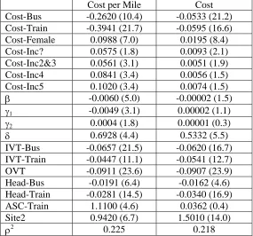
The results discussed in sections 5.2, 5.3 and 5.4 suggested a final specification for the bus-train model. The latter includes only those variables that turned out to be significant in the previous analysis. The estimation results for the final model are reported in Table 5.2.

Although the non-normalised model is reported, this is only for reference and we focus our attention on the normalised model which has a better goodness of fit and is far superior in terms of income effects and variations in the sensitivity to cost changes.

[image:16.595.76.361.114.380.2]

Table 5.2: Final Bus-Train Mode Choice Model

Cost per Mile Cost

Cost-Bus -0.2620 (10.4) -0.0533 (21.2)

Cost-Train -0.3941 (21.7) -0.0595 (16.6)

Cost-Female 0.0988 (7.0) 0.0195 (8.4)

Cost-Inc? 0.0575 (1.8) 0.0093 (2.1)

Cost-Inc2&3 0.0561 (3.1) 0.0051 (1.9)

Cost-Inc4 0.0841 (3.4) 0.0056 (1.5)

Cost-Inc5 0.1020 (3.4) 0.0074 (1.5)

β -0.0060 (5.0) -0.00002 (1.5)

γ1 -0.0049 (3.1) 0.00002 (1.1)

γ2 0.0004 (1.8) 0.00001 (0.3)

δ 0.6928 (4.4) 0.5332 (5.5)

IVT-Bus -0.0657 (21.5) -0.0620 (16.7)

IVT-Train -0.0447 (11.1) -0.0541 (12.7)

OVT -0.0911 (23.6) -0.0907 (23.9)

Head-Bus -0.0191 (6.4) -0.0162 (4.6)

Head-Train -0.0281 (14.5) -0.0340 (16.9)

ASC-Train 1.1100 (4.6) 0.0362 (0.4)

Site2 0.9420 (6.7) 1.5010 (14.0)

ρ2 _{0.225 0.218}

Note: Inc2&3 denotes £5-15,000, Inc4 denotes £15-20,000 and Inc5 denotes £20-25,000. Inc? is for those who did not income data. β, γ1, γ2 and δ are as defined in Table 5.1.

6.

THE STATED PREFERENCE EVIDENCE AND ELASTICITY VARIATION

This research was intended to complement analysis using aggregate data commissioned by DETR (Dargay and Hanly, 1999).

We now discuss the findings of the re-estimated SP models in terms of what they indicate about elasticity variation. Ideally, the results would be used to enhance analysis of the aggregate data, but even in isolation they provide an insight into expected variation in bus fare elasticities. This is discussed in section 6.1. In section 6.2, we discuss our results in the specific context of the issues analysed by Dargay and Hanly (1999) and, where possible, compare the findings of the two studies.

6.1

Variations in Sensitivity to Cost

We have been careful to use the term sensitivity to cost variations rather than cost elasticity in our discussions so far. This is because in a logit model, the implied elasticity is influenced by the sensitivity to cost as one factor amongst others. In the logit models we have developed, the implied fare elasticity for bus (ηC) would be:

)

1

(

B

B B

C

C

P

C

U

₋

∂

∂

=

η

where CB and PB are the cost of bus and the probability (market share) of choosing bus. The first term

circumstances. Two things should be noted at this point. Firstly, that the elasticity only includes the change in demand attributable to mode switching and does not include any trip generation effects. Further discussion of logit models and elasticities is provided in Appendix 4. Secondly, that this elasticity function contrasts somewhat with aggregate demand models, such as those estimated in DETR’s bus fare elasticities study, which typically have constant fare elasticities.

The logit model provides us with a means of deducing elasticities.The results we have obtained would allow the elasticities to vary with the fare level, the size and sign of bus fare changes, income levels and gender. However, it would not be appropriate to use the model to deduce absolute elasticities for the bus market. This is not only because it represents just the mode switching component of demand changes but also because our parameters are calibrated to choices between bus and train and very few bus users will have train as their best alternative. Elasticities are clearly dependent upon the attractiveness of the alternatives open to the individual.

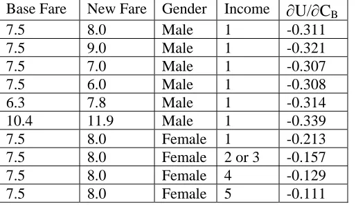
[image:17.595.73.330.367.515.2]

However, the model does provide an indication of relative elasticities if we take the results that we have obtained to be generally representative of bus users’ sensitivity to cost changes. Table 5.3 provides some representative cost coefficients given the results presented in Table 5.2 for the normalised model. The mean fare per mile in the data set is 7.5 pence, with 25 and 75 percentiles of 6.3 and 10.4.

Table 5.3: Sensitivity to Cost (

∂

U/

∂

C

B

) for Normalised Model

Base Fare New Fare Gender Income

∂

_U/

∂

_C

_B

7.5 8.0 Male 1 -0.311

7.5 9.0 Male 1 -0.321

7.5 7.0 Male 1 -0.307

7.5 6.0 Male 1 -0.308

6.3 7.8 Male 1 -0.314

10.4 11.9 Male 1 -0.339

7.5 8.0 Female 1 -0.213

7.5 8.0 Female 2 or 3 -0.157

7.5 8.0 Female 4 -0.129

7.5 8.0 Female 5 -0.111

The variation in the sensitivity to cost is not particularly great. The largest sources of variation are quite clearly income group and gender. The size of the fare change is a minor effect although there can be a reasonable degree of variation according to the fare level.

These figures denote relative elasticities. To convert into absolute elasticities, we need to relate these cost sensitivities to actual demand and fare changes. Hence an econometric model of bus demand could be specified as changes in demand between two points in time. For the two points in time,

∂

U/∂CB can be calculated and a parameter estimated to it relating it to the demand changes. The fare

elasticity can then be deduced given the implied relationship between demand and fare. However, this re-analysis of SP data and the aggregate econometric analysis have been conducted independently, and we are therefore left to compare the implied elasticity variation from the SP analysis with the findings reported in Dargay and Hanly (1999). It is to this that we now turn.

6.2

Comparison of SP Results with Findings of the Aggregate Econometric Study

The econometric analysis of bus demand data was conducted at two levels. One was aggregate time series data at the national level and split by region. The other was based on bus operators’ data aggregated only to the county level.

6.2.1

Results at a National and Regional Level

The national models distinguish between journey and passenger kilometres for the dependent variable. Note that our SP evidence is based on the effect of cost on whether bus is used or not for a particular journey and not on distance travelled.

For the national time series model, a constant elasticity model was preferred to a model which allows the elasticity to be proportional to the fare. We have found that there is support for fare elasticities varying with the fare level although the effect is not strong. Hence it is not surprising that Dargay and Hanly found the constant elasticity model preferable. However, the alternative to the constant elasticity model they estimated took the form:

F

e

V

=

µ

β

where V is the volume of demand and F is fare. The implied fare elasticity is βF and it can be argued that such a strong relationship between the fare elasticity and the fare level is unrealistic. At the very least, we ought to test for a weaker relationship between the fare elasticity and fare by using a more flexible function. Such a demand model would be:

λ β

µ

F

e

V

=

which would be estimated by non-linear least squares and has a fare elasticity of βλFλ. The λ parameter controls the degree of elasticity variation, with the constant elasticity version being the special case as λ tends to zero.

If this more general functional form had been estimated, we would have been able to gain a better idea of the consistency of the aggregate analysis and the SP analysis. Nonetheless, both data sets indicate that there is not a large degree of elasticity variation with respect to the fare level.

Dargay and Hanly were unable to detect any significant asymmetry of response. A contributory factor was the few instances where fares were falling. Whilst we have detected an asymmetry, it can be seen in Table 5.3 that it was very small. It is highly unlikely that, even if there had been real-world fare reductions corresponding to the observed fare increases, an aggregate model would be able to discern them.

In the analysis of the regional data, where data was pooled over time and across regions, the model where the fare elasticity is proportional to fare was preferred statistically to the constant elasticity model. Whilst such large elasticity variation is not consistent with the findings of our research, as is clear from the results in Table 5.3, the proportionality effect with fare will be reduced because separate parameters (β’s) were estimated by region. Thus variations in the β’s across regions can dampen the direct proportional relationship between the fare elasticity and fare level which would inevitably occur with this model if a single β was estimated for all regions.

[image:19.595.71.347.225.307.2]

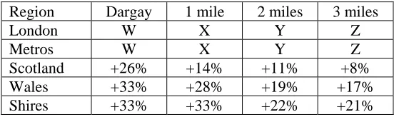
journey lengths. These are given in the final three columns. Thus the cost sensitivity for Scotland and journeys averaging 3 miles is 8% higher than for both London and the Metropolitan areas. Given that no reliable information on average journey length is provided in the report, we have converted the average fares for each region for 1990 reported by Dargay and Hanly into a pence per mile using distances of 1, 2 and 3 miles. In order to avoid having to make assumptions about income and gender, fitted cost sensitivities have not been calculated on the basis of the final bus-train model, but on the basis on the model reported in Table 5.1. The latter contains the effects only of the fare level and of the size and sign of the fare change.

Table 6.1: Regional Elasticity Variation

Region Dargay 1 mile 2 miles 3 miles

London W X Y Z Metros W X Y Z

Scotland +26% +14% +11% +8%

Wales +33% +28% +19% +17%

Shires +33% +33% +22% +21%

The pattern of results obtained in the two studies is similar, although the magnitude of the variation is higher in the Dargay and Hanly study. We have seen, however, that in the SP data income has an influence on the fare elasticities. This income effect will be automatically incorporated in the elasticity variation in the aggregate study. Whilst regional income data is not given in the report, London has above average income levels whilst Scotland and Wales are below average. It may be that allowing for income differences would lead to greater consistency in the fare elasticity variation between each study.

There was again no evidence of asymmetry of demand with respect to rising and falling prices, but a contributory factor was again that there were few instances of falling prices.

6.2.2

Results at a County Level

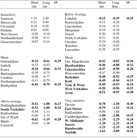
We have repeated the exercise reported in Table 6.1 to compare the fare elasticities estimated by Dargay and Hanly at the county level with our findings. We have taken the 22 elasticities in their

Table 6.2, here reproduced as our Table 6.2. which were statistically significant. Alongside these values, we report cost sensitivities derived from our models. These are given in the columns which are headed SP.

These are the results of separate constant elasticities estimated for each county in a single model. Since Dargay and Hanly argue that fare levels are the principal cause of this elasticity variation, we have again used the results in Table 5.1 to calculate cost sensitivities which depend upon the fare level. The fare levels are taken from Figure 5.5 in Dargay and Hanly, and we have converted them to pence per mile using an average distance per journey of three miles.

[image:20.595.70.513.110.559.2]

Table 6.2

Fare Elasticities for English countries. Unrestricted Constant Elasticity Model

Short run Long run SP Short run Long Run SP Insensitive Somerset Merseyside Cleveland Durham West Sussex Northumberland Gloucestershire Mean

Oxfordshire

Suffolk

Essex

Buckinghamshire Cumbria Northamptonshire

Derbyshire

Above average

Nottinghamshire

South Yorkshire Bedfordshire Isle of Wight

Hants

Cornwall 1.25 0.21 0.10 0.01 -0.05 -0.06 -0.07 -0.32 -0.33 -0.34 -0.39 -0.40 -0.41 -0.41 -0.52 -0.52 -0.58 -0.60 -0.62 -0.66 2.40 0.40 0.20 0.02 -0.10 -0.11 -0.14 -0.61 -0.63 -0.66 -0.75 -0.77 -0.79 -0.79 -1.00 -1.00 -1.11 -1.15 -1.19 -1.28 -0.29 -0.31 -0.29 -0.27 -0.24 -0.28 Below Average

London

Warwickshire Lincolnshire Shropshire Dorset North Yorkshire Cheshire Wiltshire Lancashire Mean

Gtr. Manchester

Hertfordshire Leicestershire Worcestershire Berkshire Kent

Tyne & Wear West Yorkshire Avon Very sensitive

Devon

East Sussex Staffordshire

Cambridgeshire

W. Midlands Surrey Humberside Norfolk -0.15 -0.15 -0.16 -0.19 -0.20 -0.21 -0.24 -0.24 -0.29 -0.42 -0.46 -0.47 -0.47 -0.48 -0.49 -0.49 -0.50 -0.51 -0.78 -0.79 -0.86 -1.08 -1.19 -1.20 -1.21 -1.61 -0.29 -0.28 -0.31 -0.36 -0.39 -0.41 -0.46 -0.45 -0.55 -0.82 -0.88 -0.90 -0.90 -0.92 -0.94 -0.93 -0.96 -0.97 -1.50 -1.52 -1.66 -2.08 -2.29 -2.32 -2.33 -3.09 -0.25 -0.26 -0.32 -0.28 -0.29 -0.33 -0.24 -0.25 -0.30 -0.30 -0.31 -0.35 -0.24 -0.34 -0.28 -0.31

Note: Figures in bold were statistically significant.

If we had compared our results with the results of the proportional elasticity model estimated by Dargay and Hanly on the basis of county level data, the elasticity variation in Dargay and Hanly’s models would far exceed that implied by our findings. This can be easily seen by comparing the results in Table 5.3 with the results for the variable elasticity model in Table 6.1 by Dargay and Hanly. The latter indicates a short run fare elasticity of –0.13 for a fare of 17 pence, of –0.42 for a fare of 56 pence and of –0.77 for a fare of £1.

A further inconsistency is that Dargay and Hanly find some evidence for asymmetry of response that is much stronger than was apparent in our analysis.

variation (resulting in estimates of long run elasticity ranging from –0.27 to –1.6), and that a more flexible function, as we outlined in section 6.2.1 above, might well have yielded elasticity variation between the two forms of model (constant elasticity and proportional elasticity) that they developed. They state that there is “no evidence of any relationship between the elasticity and income”. In contrast, we have found that income is expected to be an important influence on bus fare elasticities and that the fare level has a more moderate effect.

7. CONCLUDING

REMARKS

We have developed robust models with a number of plausible features to a large SP data set relating to bus users’ choices between their current mode and a train service.

The modelling process has allowed the sensitivity to cost to vary with the fare level, the sign and size of the fare change, journey purpose, service quality, age, gender and income. Statistically significant effects were discerned for the fare level, the size and sign of the fare changes, gender and income.

However, on the basis of the results obtained, we would not expect to find bus fare elasticities to vary greatly according to the sign and size of bus fare changes, although we would expect there to be a reasonable degree of fare elasticity variation according to the actual fare charged and considerable variation according to income level and gender.

On the basis of these results, we would expect fare elasticity to vary over time with the characteristics of the market. As real bus fares increase over time, we would expect the bus fare elasticity to increase. There is evidence that this has occurred in practice. If those with higher incomes switch to other modes, particularly car, and the average income of bus users falls, then there will be another tendency for bus fare elasticities to increase. On the other hand, if females form a larger proportion of bus users, there will be a tendency for bus fare elasticities to fall. Our results would have to be compared with actual changes that have occurred to indicate whether, on balance, the trend in bus fare elasticities would be positive, negative or broadly neutral.

To convert the estimated cost sensitivities into absolute fare elasticities, it would be necessary to enter the results into an econometric model relating changes in bus demand to changes in bus fares and other factors.

There are some inconsistencies between our results and those of the aggregate econometric modelling of Dargay and Hanly. Whilst there are many plausible and robust features of the latter analysis, and the overall elasticities are sensible and consistent between the aggregate and county data sets, there are difficulties involved in the comparing the elasticity variation implied by the two approaches:

• The Dargay and Hanly approach uses a model which in allowing the fare elasticity to vary ‘imposes’ a very strong effect

• There is a problem with the degree of precision with which some of the segmented elasticities are estimated in Dargay and Hanly. Admittedly, however, some of the parameters estimated here are not very precise.

• Additional data, particularly relating to income and gender breakdown, would be needed to provided a more detailed comparison

over time and lagged responses, but it has certain shortcoming with regard to data and the extent to which disaggregation can be undertaken.

We recommend:

• Further analysis, using the results of SP data to complement/enhance the analysis of bus demand at the more aggregate level. This would link the two areas of analysis much more than has been possible here. This should also explore the possibilities of extending this to variables other than fare.

• The conduct of SP exercises which are designed with the specific purpose of providing results to be entered into aggregate models. One issue is to more closely relate the scenarios in the SP exercise to the choice contexts and real world situations that are relevant to the elasticities being estimated in the aggregate model. For example, the SP exercise would cover the fare variations observed in the real world, as well as other variations, and would be careful to specify service quality interactions with fare in line with those in practice.

• Making use of the very valuable information contained in the National Travel Survey (NTS), which contains both time-series and cross-sectional data and is available at the disaggregate level of individual travellers. The NTS data set could make a large contribution to the estimation of demographic and regional influences. It could allow disentangling the effects of car ownership growth from the effects of trends in income and in other socio-economic variables.. Analysis of NTS data might also help to overcome collinearity problems, which can plague aggregate time series models.

• The use of any useful evidence from a wider range of sources, such as findings from economic theory or results from other studies. These inputs might assist in the estimation of ‘minor effects’ such as cross-elasticities. Also, they can help reducing the number of parameters to be directly estimated by isolating the effects of specific variables. As a consequence, they would ultimately enhance the degree of precision with which the effects of other attributes are estimated.

References

Bhat, C. (1997) Covariance Heterogeneity in Nested Logit Models: Econometric Structure and Application to Intercity Travel. Transportation Research 31B, pp.11-21.

Dargay, J.M. and Hanly, M. (1999) Bus Fare Elasticities. Prepared for the Department of the Environment, Transport and the Regions.

Hensher, D.A. (1996) A Practical Approach to Identifying the Market for High Speed Rail: A Case Study

in the Sydney-Canberra Corridor. Institute of Transport Studies, University of Sydney.

Ortuzar, J. de D. and Willumsen, L.G. (1994) Modelling Transport, Wiley, Chichester.

Preston, J. and Wardman, M. (1989a) Nottingham-Mansfield-Worksop New Rail Service Project: Report on the Stated Preference Survey. Report prepared for Nottinghamshire County Council.

Preston, J. and Wardman, M. (1989b) Nottingham LRT Study: Forecasting the Demand for a Light Rapid Transit System between Nottingham and Hucknall. Final Report of Phases Two and Three. Report prepared for Nottingham City Council

Preston, J. (1991) Analysis of Proposed Ribble Valley Rail Services. Report prepared for Lancashire County Council.

Taplin, J.H.E. (1982) Inferring Ordinary Elasticities from Choice or Mode Split Elasticities. Journal of Transport Economics and Policy 16, pp.55-63.

Toner, J.P. (1994) Estimating Elasticities with Limited Information. Technical Note 335, Institute for

Transport Studies, University of Leeds.

Wardman, M. (1997a) Disaggregate Urban Mode Choice Models: Review of British Evidence with Special Reference to Cross Elasticities. Working Paper 505. Institute for Transport Studies, University of Leeds.

Wardman, M. (1997b) Disaggregate Inter-Urban Mode Choice Models: Review of British Evidence with Special Reference to Cross Elasticities. Working Paper 504. Institute for Transport Studies, University of Leeds.

APPENDIX 1: CLITHEROE RAIL STUDY SP DESIGNS

COST

B

COST

T

IVT

B

IVT

T

OVT

B

OVT

B

HEAD

B

HEAD

T

220 240 65 15 20 20 60 60

120 120 50 20 20 20 60 60

170 160 35 25 20 20 60 60

170 160 50 15 15 20 60 60

160 80 35 20 15 20 60 60

220 200 65 25 15 20 60 60

220 160 35 15 10 20 60 60

170 160 65 20 10 20 60 60

120 80 50 25 10 20 60 60

COST COST IVT IVT OVT OVT HEAD HEAD

B T B T B B B T

170 240 35 15 AN AN 60 30

120 160 65 20 AN AN 20 30

220 240 50 25 AN AN 15 30

220 240 65 15 AN AN 15 20

170 240 50 20 AN AN 60 20

120 160 35 25 AN AN 30 20

120 300 50 15 AN AN 60 15

220 300 35 20 AN AN 20 15

170 240 65 25 AN AN 30 15

APPENDIX 2: NOTTINGHAM-MANSFIELD STUDY SP DESIGNS

Short Distance Design

COST

B

COST

T

IVT

B

IVT

T

OVT

B

OVT

B

HEAD

B

HEAD

T

60 40 30 15 15 20 AN 60

50 60 30 15 15 25 AN 60

40 65 30 15 10 25 AN 60

50 60 30 10 15 20 AN 60

40 65 30 10 15 25 AN 60

60 40 30 10 10 25 AN 60

40 65 25 15 15 20 AN 60

60 40 25 15 15 25 AN 60

50 60 25 15 10 25 AN 60

COST

B

COST

T

IVT

B

IVT

T

OVT

B

OVT

B

HEAD

B

HEAD

T

50 35 30 10 AN AN AN 30

40 40 30 10 AN AN AN 60

40 60 30 10 AN AN AN 30

40 40 25 15 AN AN AN 30

40 60 25 15 AN AN AN 60

50 35 25 15 AN AN AN 30

40 60 30 15 AN AN AN 30

50 35 30 15 AN AN AN 60

40 40 15 30 AN AN AN 30

Long Distance Designs

COST

B

COST

T

IVT

B

IVT

T

OVT

B

OVT

B

HEAD

B

HEAD

T

130 90 50 25 15 20 AN 60

115 125 50 25 15 25 AN 60

115 140 50 25 10 25 AN 60

115 125 60 45 15 20 AN 60

115 140 60 45 15 25 AN 60

130 90 60 45 10 25 AN 60

115 140 40 30 15 20 AN 60

130 90 40 30 15 25 AN 60

115 125 40 30 10 25 AN 60

COST

B

COST

T

IVT

B

IVT

T

OVT

B

OVT

B

HEAD

B

HEAD

T

115 90 60 40 AN AN AN 30

115 115 60 40 AN AN AN 60

95 115 60 40 AN AN AN 30

115 115 40 30 AN AN AN 30

95 115 40 30 AN AN AN 60

115 90 40 30 AN AN AN 30

95 115 50 35 AN AN AN 30

115 90 50 35 AN AN AN 60

115 115 50 35 AN AN AN 30

APPENDIX 3: NOTTINGHAM LRT STUDY SP DESIGN

COST

B

COST

T

IVT

B

IVT

T

OVT

B

OVT

B

HEAD

B

HEAD

T

APPENDIX 4: MODELLING APPROACH AND ELASTICITIES

MODELLING APPROACH

By far the most commonly used model to analyse discrete choice data is the logit model. Almost all of the applications of disaggregate mode choice models to urban and inter-urban travel in Great Britain have

been of the logit form and the vast majority. Some have been calibrated to Revealed Preference (RP) data,

some have been calibrated to Stated Preference (SP) data whilst others have involved joint estimation of hybrid models on both forms of data. Wardman (1997a, 1997b) provide reviews of a large amount of

British mode choice modelling evidence.

The multinomial logit model expresses the probability of using some alternative i as a function of the

utilities (V) of the k alternatives in the choice set:

∑

=

=

k

j V V

i

j i

e

e

P

1

In the case of choices between just two alternatives (1 and 2), the logit model can be expressed as:

1 2

1

1

1 V V

e

P

₋

+

=

In turn, utility is related to relevant observable variables (Xi):

)

(

_{i i} i

f

X

V

=

Ω

β

Ω is a scale factor whose purpose is to account for the effect of unobserved factors on choices and it is expressed as:

j

σ

π

6

=

Ω

where σj is the standard deviation of each alternative's unobserved effects. Relative valuations are

normally expressed in monetary terms; for example, the value of travel time savings is expressed as a

monetary equivalent of the time benefit. The marginal monetary valuation (MMV) of variable Xm for

ic im im

X

V

X

V

X

MMV

∂

∂

∂

∂

=

)

(

where c denotes cost. Given that Ω applies to both the numerator and denominator terms, the estimated

relative valuations are independent of the scale of the model.

A potentially undesirable feature of the logit model when there are more than two alternatives is the so called independence of irrelevant alternatives (IIA) property whereupon the cross elasticities are equal.

The most common means of allowing for differential substitutability between alternatives is the

hierarchical logit model (Ortuzar and Willumsen, 1994). This proceeds by way of a 'nesting structure' whereby alternatives that are more closely associated are placed in the same nest. Thus for choices

between car, rail and bus, it is typical to place rail and bus together in the lower nest and for the upper

nest to include car and the 'composite' public transport alternative. In this particular example, the probability of choosing car (Pc) would be:

C PT V V C

e

P

₋

+

=

1

1

where:

)

log(

Vt Vb

PT

e

e

V

=

θ

+

The probabilities of choosing train (Pt) and bus (Pb) would be:

t b V V c t

e

P

P

₋

+

−

=

1

1

)

1

(

and t b V V c b

e

P

P

₋

+

−

=

1

1

)

1

(

CHOICE ELASTICITIES

A useful indicator of the properties of a demand forecasting model is the elasticity of demand. Given the

logit model of equation 1 and a utility function as in equation 3, the point elasticity of demand for mode i with respect to changes in the level of variable X on mode k is:

)

(

int

k k

k k po

ik

X

D

P

X

V

−

∂

∂

=

η

The Kronecker delta (D) equals 1 if i=k and the term represents an own elasticity, else it is zero and the

term therefore represents a cross elasticity. It can be seen that a logit model's elasticities will depend not only on market share but also, in general, on the level of the variable for which the elasticity is being

calculated. If we specify the utility function as:

∑

Ω

=

m im im i

im

X

V

β

λ

the implied elasticity function is:

)

(

int

k km

km km po

ik

X

D

P

km

−

Ω

=

β

λ

λ

η

where D is again the Kronecker delta. The conventional approach constrains the λ's to be one, which

implies constant relative valuations but imposes appreciable variation in the elasticity with the respect to the level of its variable.

CHOICE AND ORDINARY ELASTICITIES

The elasticities obtained from mode choice models clearly do not account for trip generation or

suppression, that is, they allocate a fixed number of trips amongst the available modes. There are two ways in which we might deduce ordinary elasticities from the mode choice elasticities.

The first is a pragmatic approach and is that which has been most widely applied. It involves the application of the choice model to determine a new volume of demand for the mode in question to which

is added an amount to allow for trip generation. The ordinary elasticity is then calculated using this

amended volume of demand for the new situation relative to the volume of demand in the base situation. The problem with this approach is that information is required about the trip generation effect, and its

ratio with mode switching may well be variable across different situations. In addition, the generation

The second approach uses the relationship between mode choice and ordinary elasticities set out by Taplin (1982):

j

and

i

all

for

M

O

_ij

=

_ij

+

η

_j

where Oij is the ordinary demand elasticity for mode i with respect to the price of mode j, Mij is the

equivalent mode choice elasticity and ηj is the elasticity of demand for aggregate traffic with respect to

the price of mode j. It follows that a way forward in making fuller use of the results of disaggregate

choice models is to estimate ηj so that the ordinary elasticity can be inferred. Other possible approaches

are outlined by Oum et al. (1992).

An interesting discussion of the relationships between elasticities and how they can be deduced or their