A Nonlinear Controller for Flutter Suppression: from Simulation to Wind Tunnel Testing

A Nonlinear Controller for Flutter Suppression: from

Simulation to Wind Tunnel Testing

A. Da Ronch

University of Southampton, Southampton, SO17 1BJ, United Kingdom

N. D. Tantaroudas

, S. Jiffri

and J. E. Mottershead

University of Liverpool, Liverpool, L69 3GH, United Kingdom

Active control for flutter suppression and limit cycle oscillation of a wind tunnel wing section is presented. Unsteady aerodynamics is modelled with strip theory and the in-compressible two–dimensional classical theory of Theodorsen. A good correlation of the stability behaviour between simulation and experimental data is achieved. The paper focuses on the introduction of a nonlinearity in the plunge degree of freedom of an ex-perimental wind tunnel test rig and the design of a nonlinear controller based on partial feedback linearization. To demonstrate the advantages of the nonlinear synthesis on linear conventional methods, a linear controller is implemented for the nonlinear system that ex-hibits limit cycle oscillations above the linear flutter speed. The controller based on partial feedback linearization outperforms the linear control strategy based on pole placement. Whereas feedback linearization allows to suppress fully the limit cycle oscillations, the pole placement fails to achieve any significant reduction in amplitudes.

Nomenclature

b = semi–chord

Cξ, Cα = viscous damping in plunge and pitch, respectively

Cc

ξ = critical damping in plunge,2

p m Kξ

Cc

α = critical damping in pitch,2 √

IαKα

Kξ, Kα = plunge stiffness and torsional stiffness about elastic axis

Kξ3, Kξ5 = third and fifth order terms of plunge stiffness

Iα = second moment of inertia of aerofoil about elastic axis

CL, Cm = lift and pitch moment coefficients

m = aerofoil sectional mass

h = plunge displacement

k = reduced oscillation frequency,ω c /2U∞

Sα = first moment of inertia of aerofoil about elastic axis

t = physical time

xα = aerofoil static unbalance,Sα/m b

R = residual vector

ra = radius of gyration of aerofoil about elastic axis,ra2 = Iα/m b2

U∞ = freestream velocity

UL = linear flutter speed

U∗

= reduced velocity,U/b ωα

w = vector of unknowns

Wg = gust vertical velocity

∗_{Lecturer, Faculty of Engineering and the Environment; [email protected]. Member AIAA (Corresponding Author).} †_{PhD. Student, School of Engineering.}

‡_{Research Associate, School of Engineering.}

Greek

α = angle of attack

δ = trailing–edge flap deflection τ = non-dimensional time,t U∞/ b

ωξ = uncoupled plunging mode natural frequency,

p Kξ/m

ωα = uncoupled pitching mode natural frequency about elastic axis,

p Kα/Iα

¯

ω = ratio ofωξ/ωα

ζξ = damping ratio in plunge,Cξ/Cξc

ζα = damping ratio in pitch,Cα/Cαc

ξ = non–dimensional displacement in plunge,h/b

µ = mass ratio,m/π ρ b2

Symbol

( )′

= differentiation with respect toτ, d( )/dτ

I.

Introduction

Rewrite

The work detailed in this paper is part of the development of a systematic approach to flight control system design for very flexible or very large aircraft.1–3 _{In this paper, in particular, the focus is on the exploitation of}

an approach to model reduction for flutter suppression of a wind tunnel aeroelastic system. The conference manuscript will include aspects of control design based on analytical models, and the implementation and validation to extend the flutter boundary of a wing section mounted in a wind tunnel, with emphasis on the integration of numerical methods in experimental practise.

Previous work by the author has focused on gust loads prediction and alleviation using standard control techniques based on H∞ and H2. There is, however, a large number of alternative control algorithms

available, and these are briefly summarised below. While these controllers were applied for gust loads alleviation, it is desirable that the control algorithm is effective to suppress unwanted effects, e.g. flutter or limit cycle oscillation (LCO).

Active control has been widely applied in experimental investigations for flutter suppression using control surfaces4 _{and also for gust loads alleviation.}5 _{In Ref.,}6 _{the stability threshold for a two degrees of freedom}

aeroelastic system was increased by a nonlinear energy sink, based on the principle of nonlinear energy pumping. In Ref.7 _{a nonlinear controller based on feedback linearization was applied on a wind tunnel}

model with a continuous stiffening-type structural nonlinearity to suppress the vibrations. The controller implementation was also tested when an uncertainty in the nonlinear pitch stiffness was present.

Nonlinearities in aeroelastic system induce pathologies such as LCO under certain circumstances and there is limited study of the active control of these nonlinear aeroelastic systems. A linear controller can in general stabilise the nonlinear system but empirical evidence suggests that stability is not guaranteed in strongly nonlinear regimes. Reference8_{designed a nonlinear controller based on a partial feedback linearization. The}

limitation of the approach is that it depends on the exact cancellation of the nonlinearity. In Ref.,9_{a linear}

quadratic Gaussian control that takes into account a control input delay was designed and applied to control an experimental wind tunnel model for flutter suppression.

More recently, control design has been shown for stability augmentation and gust load alleviation in flex-ible aircraft.10 _{A common approach is to fully account for the nonlinear structural behaviour while simple}

linear aerodynamic models based on two-dimensional theory and panel methods were used for the aerody-namics. Some attempts applied adaptive and nonlinear control techniques in aeroelastic systems. Recent advances in adaptive control and especially in L1 adaptive control theory made possible the application of adaptive controllers for the control of uncertain nonlinear systems.11 _{This design uses a state predictor}

have been applied at a flexible aircraft problem by using a rigid aircraft as a reference model and a neural network adaptation to control the structural flexible modes and to compensate for the effects of unmodeled dynamics.15

The paper continues in§ IIwith a description of the aeroelastic wind tunnel test rig. Then, the numerical model used in this work is detailed in §III. Feedback linearization is presented in §IV, followed by an overview of experimental and numerical results in §V. Finally, conclusions are given.

II.

Wind Tunnel Nonlinear Aeroelastic Test Rig

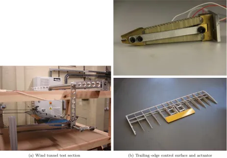
A flexible wing section was tested in the University of Liverpool wind tunnel. This tunnel has a maximum operating speed of around 20 m/s, which is well above the designed flutter speed of the model. The wing section in Fig. 1is mounted horizontally and is supported by adjustable vertical and torsional leaf springs. The wing section consists of a NACA 0018 aerofoil, with a chord of 0.35 m and a span of 1.2 m. The total mass of the system is around 6.5 kg. The control surface is driven by a V–stack piezoelectric actuator, and the maximum deflection is ±7 deg. Two laser sensors are mounted externally to the working section to measure the displacements of two points attached to the aerofoil shaft. The pitch and plunge degrees of freedom are readily available from these measurements. Preliminary tests were made to guarantee that the flexible modes of the wing, e.g. spanwise bending modes, are well above the pitch and plunge frequencies, and a separation of over one order magnitude was found. More details on the (linear) baseline aeroelastic wind tunnel model were presented in Ref.16

(a) Wind tunnel test section (b) Trailing–edge control surface and actuator

Figure 1. Schematic view of the experimental setup of the aeroelastic model in the University of Liverpool

The experimental rig was then modified to introduce a concentrated hardening nonlinearity in the plunge degree of freedom. The design follows Ref.17 _{The nonlinearity in the restoring force on each end of the}

aerofoil is realised by a clamped cable under tension, which acts as a hardening spring. Figure2shows the system of cables used to introduce the nonlinearity in the wind tunnel rig.

Figure 2. Schematic view of the system of cables used to introduce a nonlinearity in the wind tunnel test rig (from Ref.17

)

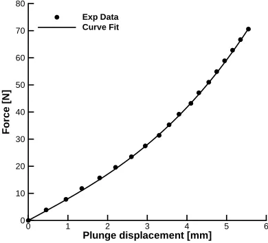
passing over the pulleys on both sides of the aerofoil. Thus, the strength of the nonlinearity is adjusted as required. At present, a weight of 2 kg is hung on each side, and the force–deflection profile was found by applying known, equal, downward loads at each end of the aerofoil and measuring the deflection. A non–contact laser displacement sensor was used to measure deflection. Figure3 shows the measured points for the nonlinear case along with a polynomial fit. The nonlinear relation between vertical force and plunge displacement is formulated as

Fnl = Kξh+ Kξ3h 3 _{+ K}

ξ5h

5 ₍₁₎

where the stiffness constantsKξ = 7.886·103N/m, Kξ3= 1.603·10

8 _N/m3_{, andK}

ξ5=−8.226·10

10_N/m5

were calculated by a least–squares fit.

Plunge displacement [mm]

F

o

rc

e

[

N

]

0 1 2 3 4 5 6

0 10 20 30 40 50 60 70 80

Exp Data Curve Fit

Figure 3. Structural nonlinearity in plunge displacement measured experimentally

III.

Aeroelastic Model

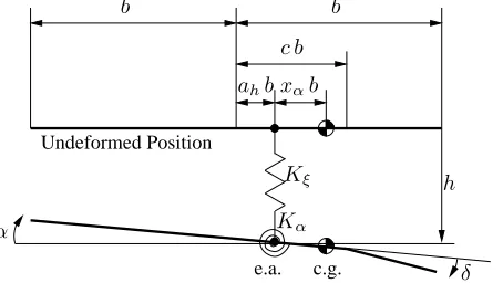
about the elastic axis, positive with nose up. The motion is restrained by two springs,Kξ andKα, and is

assumed to have a horizontal equilibrium position ath = α = 0. Structural damping in both degrees of freedom is also included in the system. A trailing-edge flap, which is assumed massless in this study, is used in combination with an active control system to extend the stable flight region and for gust loads alleviation.

Undeformed Position

e.a. c.g. ahb xαb

α

Kξ

Kα

δ c b

b b

h

Figure 4. Schematic of a two-degree of freedom aeroelastic system; the wind velocity is to the right and horizontal

The motion of the system, without control surface dynamics and with a linear structural model, is described in non–dimensional form by

"

1 xα

r2

α

xα 1

# ( ξ′′

α′′

) +

" _2ζ

ξω¯

U∗ 0

0 2ζαω¯

U∗ # (

ξ′

α′

) +

" ¯

ω U∗

2 0 0 1

U∗ 2

# ( ξ α

) =

(

−π µ1 CL(τ)

2

π µ r2

aCm(τ)

) (2)

The lift coefficient,CL, is defined positive upward according to the usual sign convention in aerodynamics.

The plunge displacement is positive downward. Hence, the negative sign in front ofCL in Eq. (2). Non–

dimensional parameters are defined in the nomenclature. Note also that the above equations are formulated in terms of a non–dimensional time,τ, based on the aerofoil semi–chord and freestream speed,τ=t U∞/b.

The above model of the pitch–plunge aerofoil system, with an appropriate model of the aerodynamics, is used in this work to simulate the dynamics of the wind tunnel nonlinear aeroelastic test rig.

III.A. Two–dimensional Thin Aerofoil Theory

Several options for the aerodynamics can be used. For an irrotational and incompressible two–dimensional flow, the aerodynamic model is given by the classical theory of Theodorsen. This is a reasonable assumption because of the low–speed characteristics of the wind tunnel used in this work.

The total aerodynamic loads consist of contributions arising from the section motion (pitch and plunge), flap deflection, and the penetration into a gusty field. The aerodynamic loads due to an arbitrary input time–history are obtained through convolution against a kernel function. Since the assumption is of linear aerodynamics, the effects of the various influences on the aerodynamic forces and moments are added together to find the variation of the forces and moments in time for a given motion and gust

CL(τ) = CLm +C f L +C

g L

Cm(τ) = Cmm +Cmf +Cmg

III.A.1. Influence of aerofoil motion

The resulting force and moment coefficients for any arbitrary aerofoil motion in pitch and plunge are formu-lated as

Cm

L (τ) =π(ξ ′′

(τ)− ahα ′′

(τ) + α′

(τ)) +

2πα(0) + ξ′

(0) + (1/2 − ah)α ′

(0)φw(τ) +

2π Z τ

0

φw(τ−σ)

α′

(σ) + ξ′′

(σ) + (1/2 −ah)α′′(σ)

dσ (3)

Cm

m(τ) =π(1/2 + ah)

α(0) + ξ′

(0) + (1/2 ₋ah)α′(0)

φw(τ) +

π(1/2 + ah)

Z τ

0

φw(τ−σ)

α′

(σ) + ξ′′

(σ) + (1/2 −ah)α ′′

(σ)dσ+ π

2ah(ξ

′′

(τ) ₋ ahα ′′

(τ)) ₋(1/2 ₋ ah)

π 2 α

′

(τ) ₋ π 16α

′′

(τ) (4)

The Wagner function, φw, accounts for the influence of the shed wake, and is known exactly in terms of

Bessel functions. For a practical evaluation of the integral, the exponential approximation of Jones18_{is used}

φw(τ) = 1 − Ψ1e −_ε1τ

− Ψ2e−_ε2τ

(5)

where the constants areΨ1 = 0.165,Ψ2 = 0.335,ε1 = 0.0455, andε2 = 0.3.

III.A.2. Influence of trailing–edge flap rotation

The increment in aerodynamic loads for any arbitrary trailing–edge flap motion depends on the rotation, angular velocity, and acceleration through the following relations

C_Lf(τ) = ₋T4δ

′

(τ) ₋ T1δ

′′

(τ) +

2π ₁

πT10δ(0) + 1 2πT11δ

′

(0)

φw(τ) +

Z τ

0 ₁

πT10δ

′

+ 1 2πT11δ

′′

φw(τ − σ)dσ

(6)

Cf

m(τ) = −

(T4 + T10)

2 δ(τ) −

T1 −T8 −(c − ah)T4 + 1₂T11

2 δ

′

(τ) + (T7 + (c −ah)T1)

2 δ

′′

(τ) +

π(ah + 1/2)

1

πT10δ(0) + 1 2πT11δ

′

(0)

φw(τ)) +

Z τ

0

1 πT10δ

′

+ 1 2πT11δ

′′

φw(τ − σ)dσ

(7)

III.A.3. Influence of gust encounter

For the response to an arbitrary gust, the lift and pitching moment coefficients can be computed from

C_Lg(τ) = 2π U∗

Wg(0) Ψk(τ) +

Z τ

0

Ψk(τ−σ)

d Wg

dσ dσ

(8)

Cg m(τ) =

π

U∗ (1/2 +ah)

Wg(0) Ψk(τ) +

Z τ

0

Ψk(τ−σ)

d Wg

dσ dσ

(9)

The integration uses the exponential approximation of the Küssner function

Ψk(τ) = 1 − Ψ3e −ε3τ

−Ψ4e−ε4τ

(10)

III.B. Residual Formulation

The coupled system of equations resulting from combining Eq. (2) with the aerodynamic loads is integro– differential. It is difficult to study the dynamic behaviour of the system analytically. In addition, most of the methods for studying nonlinear systems are developed for ordinary differential equations. The mathematical procedure to avoid the convolution integral term has been applied to several systems in the literature. It is essentially based on defining additional variables and equations describing their evolution.

Following the approach of Ref.,20_{the system of integro–differential equations is recast as a set of ordinary}

differential equations in first order by defining eight aerodynamic states and their dynamicsa

w1(τ) = Z τ

0

e−ε1(τ−σ)_{α(σ)dσ, w}′

1(τ) = α(τ) −ε1w1(τ)

w2(τ) = Z τ

0

e−_ε2(τ−_σ)_{α(σ)dσ, w}′

2(τ) = α(τ) −ε2w2(τ)

w3(τ) = Z τ

0

e−ε1(τ−σ)_{ξ(σ)dσ, w}′

3(τ) = ξ(τ) − ε1w3(τ)

w4(τ) = Z τ

0

e−ε2(τ−σ)_{ξ(σ)dσ, w}′

4(τ) = ξ(τ) − ε2w4(τ)

w5(τ) = Z τ

0

e−ε1(τ−σ)_{δ(σ)dσ, w}′

5(τ) = δ(τ) − ε1w5(τ)

w6(τ) = Z τ

0

e−_ε2(τ−_σ)_{δ(σ)dσ, w}′

6(τ) = δ(τ) − ε2w6(τ)

w7(τ) = Z τ

0

e−ε3(τ−σ)_W

g(σ)dσ, w ′

7(τ) = Wg(τ) −ε3w7(τ)

w8(τ) = Z τ

0

e−ε4(τ−σ)_W

g(σ)dσ, w8′ (τ) = Wg(τ) −ε3w8(τ)

The size of the coupled aeroelastic model is 12, and consists of 8 aerodynamic states and 4 structural states. The trailing–edge flap rotation is used as control input. In the results presented in this work, it is assumed that the gust disturbance is null. Define the state vector (of dimension 12),

x = (α, α′

, ξ, ξ′

, w1, w2, w3, w4, w5, w6, w7, w8)T (12)

then, the coupled system of equations is

x′

1 = x2 x′

2 = p1H(x) + p2P (x) x′

3 = x4 x′

4 = p3H(x) + p4P(x) x′

5 = x1 −ε1x5 x′

6 = x1 −ε2x6 x′

7 = x3 −ε1x7 x′

8 = x3 −ε2x8 x′

9 = δ −ε1x5 x′

10 = δ −ε2x6 x′

11 = Wg −ε3x11 x′

12 = Wg −ε4x12 a

A useful tool for the calculation ofw′

j, forj = 1, . . . ,8, is the Leibniz integral role: 21

∂ ∂z

Zb(z)

a(z)

f(x, z)dx =

Z b(z)

a(z)

∂ f

∂z dx+f(b(z), z) ∂ b

∂z −f(a(z), z) ∂ a

where the dependence on time, τ, was omitted for brevity. It is convenient for the remaining part of this work to recast the above set of equations in a matrix–vector form

x′

(τ) = f(x, τ) + gu(τ) (13)

wheref(x)is a nonlinear function of the state vector,x, andurepresents the flap rotation,δ(dependence on time added).

The coefficients of the above aeroelastic system are detailed fully in the Appendix at the end of this manuscript. This allows to setup the numerical model starting from the baseline aeroelastic parameters of the pitch–plunge aerofoil described.

IV.

Control Strategies

Two control strategies based on pole placement and feedback linearization are used in this work. A detailed derivation of the feedback linearization is now presented.

IV.A. Feedback Linearization

Feedback linearization22,23_{is a widely used method in the control of nonlinear systems. The method is based}

on providing a nonlinear feedback to the system that effectively eliminates the nonlinearity and also applies a linear control strategy, such as pole placement. This method is used to control the nonlinear aeroelastic model detailed above.

In the work presented in this study, the gust disturbance is considered null. The trailing–edge flap rotation,δ, is the control input to the system. The nonlinear state space form of Eq. (13) is restated as

x′

(τ) = f(x, τ) + gu(τ)

where

f(x) =

                                                                 x2   

λ1x1 + λ2x2 +λ3x3 +λ4x4 +λ5x5 + λ6x6+

λ7x7 + λ8x8 + λ9x9 + λ10x10 + λ11x11 +λ12x12 +λ1,3x31+ λ3,3x33 +λ1,5x51 + λ3,5x53 +λδ′δ′ +λ_δ′′δ′′

   x4   

γ1x1 +γ2x2 +γ3x3 +γ4x4 +γ5x5 +γ6x6+

γ7x7 +γ8x8 +γ9x9 +γ10x10 +γ11x11 + γ12x12 + γ1,3x31+ γ3,3x33 + γ1,5x15 +γ3,5x53 + γδ′δ

′

+ γδ′′δ

′′



 

x1 − ǫ1x5 x1 − ǫ2x6 x3 − ǫ1x7 x3 − ǫ2x8

−ǫ1x9

−ǫ2x10

−ǫ3x11

−ǫ4x12

                                                                

,g=                                                0 λδ 0 γδ 0 0 0 0 1 1 0 0                                                (14)

and u=δ. Note that these equations treat δ, the flap angle, as the only input to the system, whereas its time–derivatives, δ′

and δ′′

, are treated as time–varying quantities which are part of the system. They are neither inputs nor state variables. The termsδ′

andδ′′

may be computed at each time step using a backward Euler finite difference method, using the values ofδ for the present and previous time instants. The terms λandγarise from the linear combinations of rows 2 and 4 from Eq. (13).

IV.B. Pitch Output Linearization

single output is also chosen. Choosing the pitch degree of freedom as an output(Q1: do we really need to use the symbolyαand its time derivatives; Q2: replace in z the( )˙ with( )′ for consistency)

z1 = yα = x1 (15)

Note that this output also forms the first co–ordinate,z1, in the linear domain. Following the standard input–output linearization procedure, the above expression is repeatedly differentiated until the input term appears, whilst substituting from Eq. (14) at each stage.

z2 = ˙z1 = ˙yα = ˙x1 = x2 (16)

and

˙

z2 = ¨yα = ˙x2 = 

 

λ1x1 +λ2x2 + λ3x3 + λ4x4 +λ5x5 +λ6x6+ λ7x7 +λ8x8 +λ9x9 +λ10x10 +λ11x11 +λ12x12 +λ1,3x31+

λ3,3x33 + λ1,5x51 +λ3,5x53 + λδ′δ′ + λ

δ′′δ′′





 + λδu (17)

Denoting the above equation concisely as

˙

z2 = ¨yα = ˙x2 = f2(x) + λδu (18)

the system in linear co–ordinates can be formulated as

( ˙ z1

˙ z2

) =

" 0 1 0 0

# ( z1 z2

) +

( 0 1

)

να (19)

and the actual nonlinear control input is

u = (να−f2(x)) λδ

(20)

The artificial inputναcan be used to design a controller to achieve pole–placement, which is the objective

in the present work. In this case,να will take the form

να = −g1z1 − g2z2 (21)

whereg1andg2 are appropriately chosen controller gains. The actual inputuwill then implement this pole placement, while simultaneously eliminating the nonlinearity.

It is evident from Eq. (19) that the linearised sub–system has dimension 2. Since the dimension of the full system is 12, an un–linearised portion known as the internal dynamics remains of dimension 10. Stability of the internal dynamics is a pre–requisite for overall stability of the closed–loop system. This in turn can be ensured by verifying the stability of the zero–dynamics found by setting to zero the co–ordinates corresponding to the linearised sub–system (in this casez1andz2) in the internal dynamics expressions. The latter may be chosen arbitrarily, such that the derivatives of each co–ordinate with respect toxis orthogonal to g, resulting in the normal form of the equations being acquired (in the normal form, the system inputs will not appear in the internal dynamics equations, making the zero–dynamics uncontrollable).

The transformation between the nonlinear and linear domains,Tzx, is given by

where

Tzx =

                       

1 0 0 0 0 0 0 0 0 0 0 0 0 1 0 0 0 0 0 0 0 0 0 0 0 0 1 0 0 0 0 0 0 0 0 0 0 −γδ

λδ 0 1 0 0 0 0 0 0 0 0

0 0 0 0 1 0 0 0 0 0 0 0 0 0 0 0 0 1 0 0 0 0 0 0 0 0 0 0 0 0 1 0 0 0 0 0 0 0 0 0 0 0 0 1 0 0 0 0 0 −λ1δ 0 0 0 0 0 0 1 0 0 0

0 −λ1δ 0 0 0 0 0 0 0 1 0 0

0 0 0 0 0 0 0 0 0 0 1 0 0 0 0 0 0 0 0 0 0 0 0 1

                        (23)

Using this transformation, the zero dynamics is derived as

                   ˙ z3 ˙ z4 ˙ z5 ˙ z6 ˙ z7 ˙ z8 ˙ z9 ˙ z10 ˙ z11 ˙ z12                    zd =                    z4

−γδ

λδf2(z) + f4(z)

−ǫ1z5

−ǫ2z6 z3 −ǫ1z7 z3 −ǫ2z8

−λ1δf2(z) −ǫ1z9

−λ1δf2(z) −ǫ2z10

−ǫ3z11

−ǫ4z12

                   zd (24)

where f2(z),f4(z) in the above equation are the second and fourth rows off(x)in Eq. (14), specified in terms of z, with z1 = z2 = 0. It is evident that the zero–dynamics are nonlinear, and one must ensure their stability in order to verify the feasibility of the controller in Eq. (20)(Q: was this verified and how?).

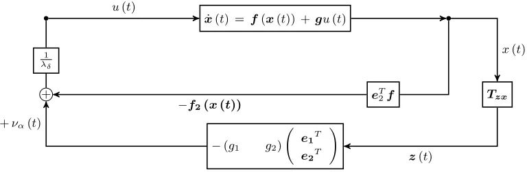
The implementation of the nonlinear controller is shown in the block diagram of Fig.5. The termse₁,e₂

indicate the first and second columns, respectively, of a12_×12identity matrix.

˙

x(t) = f(x(t)) +gu(t)

1

λδ

+ eT

2f Tzx

−(g1 g2)

e1T

e2T !

u(t)

z(t) +να(t)

−f2(x(t))

x(t)

Figure 5. Nonlinear control block diagram

IV.C. A note on Plunge Output Linearization

The aerodynamic states, on the other hand, are not measured directly and they depend on the aerodynamic model used. The clear choice is to use either the pitch or the plunge degrees of freedom. For the aeroelastic model setup considered in this work, it transpires that the zero–dynamics for the plunge control are unstable, ruling out the possibility of plunge control.

V.

Results

Validation results of the codeb_{used in this work have been reported elsewhere}1–3_{and will not be discussed}

here. The stability analysis of the linear aeroelastic model is first predicted and compared with a set of data available from wind tunnel measurements. This is followed by simulation results for the nonlinear aeroelastic model that are presented for both open– and closed–loop cases.

V.A. Stability Analysis of the Linear Aeroelastic Test Rig

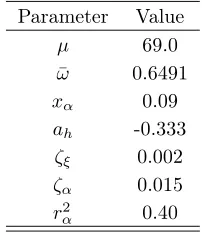
The numerical model was first validated against available wind tunnel measurements for the (linear) baseline aeroelastic wind tunnel rig. The aeroelastic parameters are summarised in Table1. For scaling to dimensional units, the constantsωα= 35.3540rad/s and b= 0.175m were used. A comparison in terms of eigenvalues tracing is illustrated in Fig.6 for increasing freestream speed. The analytical results were obtained solving for each freestream speed an eigenvalue problem of the coupled full order model. For the wind tunnel data, measurements of the frequency response functions (FRF) were obtained by a stepped–sine forced motion of the control surface. Since the FRFs relate the input voltage applied to a power amplifier of the V– stack piezoelectric actuator to the output displacements of two points attached with the aerofoil shaft, the dynamics of the system as well as the dynamics of actuators/sensors are included in the measurements.

Table 1. Aeroelastic parameters of the (linear) baseline aeroelastic wind tunnel rig

Parameter Value

µ 69.0

¯

ω 0.6491

xα 0.09

ah -0.333

ζξ 0.002

ζα 0.015

r2

α 0.40

Analytical results are in good agreement with tunnel measurements. For increasing freestream speed, the damping of the coupled system increases. At the flutter point, which occurs for a speed of UL = 17.63

m/s, the damping ratio becomes negative and a coalescence of the pitch and plunge frequencies is observed. The predicted flutter speed compares well with the value of about 17.5 m/s extrapolated using the flutter margin method24 _{from available measurements. This value, however, is extrapolated from data at lower}

speeds (between 6 and 15 m/s) and is affected by uncertainties.

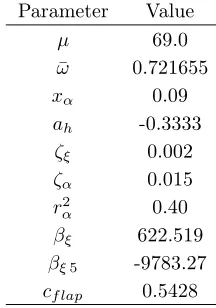
V.B. Open–loop Simulations of the Nonlinear Aeroelastic Test Rig

The aeroelastic parameters of the nonlinear aeroelastic wind tunnel test rig are summarised in Table 2. Results considered in the remaining of this paper are for this nonlinear configuration. The non–dimensional stiffness coefficients that describe the structural nonlinearity, βξ and βξ5, were obtained by converting the

coefficientsKξ,Kξ3, andKξ5in Eq. (1) in the non–dimensional form in which the aeroelastic system equations are expressed.

Add speed vs LCO amplitude plot.

The linear flutter speed of the nonlinear aeroelastic system is found at 16.24 m/s. Thus, the freestream speed for the simulation is chosen to be slightly above this value, at 17 m/s. An initial conditionα0 = 5deg is prescribed, and the simulation is run for a total time of 5 s. The resulting open–loop response is plotted

b

Wind speed [m/s]

F

re

q

u

e

n

c

y

[

H

z]

0 5 10 15 20

2 3 4 5 6 7

Simulation Wind Tunnel

(a) Damped frequency,ωd

Wind speed [m/s]

D

a

m

p

in

g

R

a

ti

o

[

%

]

0 5 10 15 20

-.1 0 .1 .2 .3 .4

Simulation Wind Tunnel

(b) Damping ratio,ζ

Figure 6. Eigenvalues tracing for varying freestream speed from simulation and wind tunnel measurements for the (linear) baseline test rig

Table 2. Aeroelastic parameters of the nonlinear aeroelastic wind tunnel rig

Parameter Value

µ 69.0

¯

ω 0.721655

xα 0.09

ah -0.3333

ζξ 0.002

ζα 0.015

r2

α 0.40

βξ 622.519

βξ5 -9783.27 cf lap 0.5428

in Fig.7. The nonlinear model above the flutter speed exhibits limit cycle oscillations. This is attributed to the fact that the structural nonlinearity acts as a hardening spring and prevents the aeroelastic response to become unstable. The response can be eliminated by applying feedback linearization, and the poles of the linearised system set as desired.

V.C. Closed–loop Simulations using Pole Placement

Before designing a nonlinear controller, a linear implementation for performance comparison is investigated. In the case considered in this paper, a pole placement technique based on a pole placement algorithm first presented in Ref.25 _{was used to add damping to the eigenvalue associated with the pitching mode and the}

linear controller was integrated together with the nonlinear system dynamics. The open– and closed–loop eigenvalues of the system for these flow conditions are shown in Table 3. (... say from x to y in terms of frequency and damping for the open and closed)

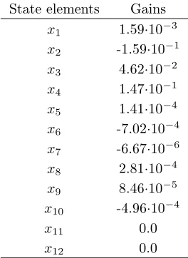
The necessary control feedbackK(symbol not used before)to achieve the specified closed loop eigenvalues in Table.3is given in non–dimensional values in Table4.

Time [s]

P

it

c

h

a

n

g

le

(

d

e

g

)

0 1 2 3

-15 -10 -5 0 5 10 15

Linear Nonlinear

(a) Pitch angle

Time [s]

P

lu

n

g

e

d

is

p

l

[m

]

0 1 2 3

-.04 -.02 0 .02 .04

Linear Nonlinear

(b) Plunge displacement

Figure 7. Open–loop time–domain response comparison between the linear and nonlinear aeroelastic models (U∞= 17.0

m/s,α0= 5.0deg); for the linear model,βξandβξ5 are set to zero

Table 3. Open– and closed–loop eigenvalues [rad/-]Q: need to show aerodynamic eigenvalues?

Open–loop Closed–loop -0.0586±0.3049i -0.0162±0.0626i

0.0061±0.2927i 0.0061±0.2927i

-0.2755 -0.2755

-0.3000 -0.3000

-0.0432 -0.0432

-0.0455 -0.0455

-0.0455 -0.0455

-0.3000 -0.3000

Table 4. Feedback gains for pole placementQ: feedback on aerodynamic states? very unrealistic

State elements Gains x1 1.59·10−3 x2 -1.59·10−1 x3 4.62·10−2 x4 1.47·10−1 x5 1.41·10−4 x6 -7.02·10−4 x7 -6.67·10−6 x8 2.81·10−4 x9 8.46·10−5 x10 -4.96·10−4

x11 0.0

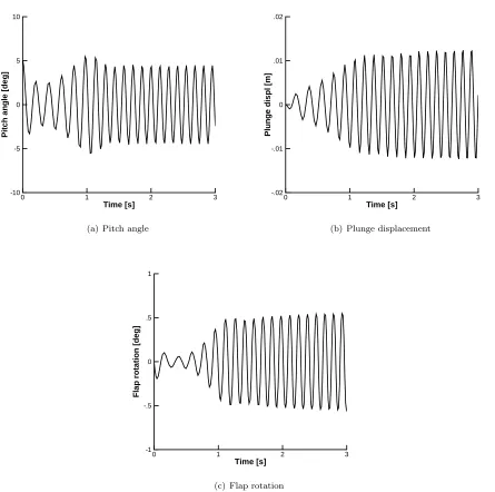
for flutter suppression is tested by keeping this unstable mode and separating the pitch from the plunge mode by moving the pitch eigenvalue.

The closed–loop response of the nonlinear system in this case is given in Fig.8. (Q1: add open–loop for comparison; Q2: regenerate time response with smaller time step, not smooth at the moment). The system exhibits LCO under the linear controller implementation and this can be confirmed also by the time history of the required flap rotation. As a result one can assume that the nonlinear system cannot be stabilised by keeping this unstable plunging mode and move only the pitching mode as the unstable plunging mode becomes dominant of the system’s response.

Time [s]

P

it

c

h

a

n

g

le

[

d

e

g

]

0 1 2 3

-10 -5 0 5 10

(a) Pitch angle

Time [s]

P

lu

n

g

e

d

is

p

l

[m

]

0 1 2 3

-.02 -.01 0 .01 .02

(b) Plunge displacement

Time [s]

F

la

p

r

o

ta

ti

o

n

[

d

e

g

]

0 1 2 3

-1 -.5 0 .5 1

(c) Flap rotation

Figure 8. Closed–loop time–domain response of the nonlinear aeroelastic model using pole placement (U∞= 17.0m/s,

α0= 5.0deg)

V.D. Closed–loop Simulations using Partial Feedback Linearisation

to say it before as commented above). In fact, it is found that the underlying linear system of Eq. (24) is also stable, as the real parts of all eigenvalues are negative. Thus, one may conclude that partial feedback linearization of the aeroelastic model based on pitch output is feasible.

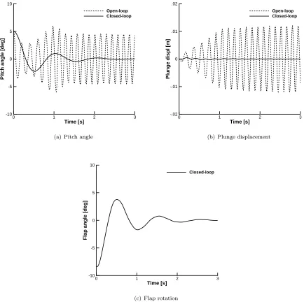
The pole–placement requirement is set to assign a natural frequency of 1 Hz, and a damping ratio of 0.25 to the pitch mode, resulting in a closed–loop pole of -0.01617±0.06263i. In the linear version of the open–loop system, these quantities were 4.8 Hz and 0.1886 respectively, with the open-loop pole of the pitch mode being₋0.05855_±0.3049i. say this earlier - perhaps a common subsection and two subsubsections for pole placement and pfl. Subsequently, the required controller gains,g1 andg2, are found as 4.18·10−3rad, 3.23·10−2 _{rad, respectively, and the artificial input computed according to Eq. (21). Assuming knowledge} of the system nonlinearity, and also availability of the other state variables, the actual nonlinear input, e.g. flap rotation, may then be computed using Eq. (20). The resulting closed–loop response is shown in Fig.9.

Time [s]

P

it

c

h

a

n

g

le

[

d

e

g

]

0 1 2 3

-10 -5 0 5 10

Open-loop Closed-loop

(a) Pitch angle

Time [s]

P

lu

n

g

e

d

is

p

l

[m

]

0 1 2 3

-.02 -.01 0 .01 .02

Open-loop Closed-loop

(b) Plunge displacement

Time [s]

F

la

p

a

n

g

le

[

d

e

g

]

0 1 2 3

-10 -5 0 5 10

Closed-loop

(c) Flap rotation

Figure 9. Closed–loop time–domain response of the nonlinear aeroelastic model using partialfeedback linearization (U∞= 17.0m/s,α0= 5.0deg)

the (uncontrolled) plunge mode also decays to zero, as do the remaining (aerodynamic) uncontrolled states, which is a reflection of the stability of the internal dynamics for this particular choice of control output.

VI.

Conclusions

This paper extends previous work done on a wind tunnel aerofoil test rig at the Universty of Liverpool. A concentrated hardening nonlinearity has now been incorporated into the originally linear aeroelastic system, which gives rise to limit cycle oscillations when the system is simulated above its linear flutter speed. Two methods of controlling flutter have been simulated, both of which seek to implement pole–placement. In the first method, the nonlinearity was not incorporated in the design of the controller, and the control law thus designed was implemented on the nonlinear system. In contrast, the second method based on partial feedback linearization implemented a nonlinear control law that eliminated the nonlinearity from a chosen output and applied the desired pole–placement on a sub–system composed of this output. A comparison of the closed–loop response in both cases revealed that whilst a marginal improvement in response was evident in the first case, the nonlinear controller was able to eliminate the limit cycle oscillations, assign the desired poles to the pitch output and drive the response of the closed–loop system to the origin.

Whilst the application of feedback linearization to an aeroelastic system is in itself not new, the present work stems from a more detailed aeroelastic model than has been done in similar previous work. Thus, the possibilities for implementing this control using the numerical model in conjunction with the wind–tunnel rig are exciting, and are hoped to yield valuable insight into control of nonlinear aerolastic systems.

Appendix

The coefficients of the coupled aeroelastic model that is used in this work are detailed below. The four coefficients determining the dynamics of the pitch and plunge degrees of freedom in Eq. (13) are formulated as

p1 = c0 (d0c1 −c0d1)

, p2 = −d0 (d0c1 −c0d1)

p3 = −

c1 (d0c1 −c0d1)

, p4 =

d1 (d0c1 −c0d1)

The nonlinear dependency of the coefficientsH(x)andP(x)on the state vector is attributed to the struc-tural model. For a polynomial form, as assumed in this work, the termH(x)is

H(x) =d2x2 +d3x1 + d4x31 + d41x51 +d5x4 + d6x3 +d7x5+

d8x6 +d9x7 + d10x8 + d11x9 +d12x10 + d13x11 +d14x14 −gf

andP(x)is

P(x) =c2x4 + c3x2 +c4x3 + c5x33 + c51x53 + c6x1 + c7x5+

c8x6 + c9x7 + c10x8 +c11x9 +c12x10 +c13x13 +c14x14 −ff

βξ5,βα,βα5

c0 = 1 + 1

µ, c1 = xα − ah

µ, c2 =

2ζξ

¯ ω U∗ +

2

µ(1 − Ψ1 −Ψ2)

c3 =

1 µ +

2

µ(1/2 − ah) (1 −Ψ1 − Ψ2)

, c4 = ω¯

U∗

2 + 2

µ(ε1Ψ1 + ε2Ψ2)

c5 = ω¯

U∗

2

βξ, c51 = ω¯

U∗

2 βξ5

c6 = 2 µ

(1 −Ψ1 −Ψ2) + (1/2 −ah) (ε1Ψ1 + ε2Ψ2)

, c7 = 2

µε1Ψ1 (1 −ε1 (1/2 −ah))

c8 = 2

µε2Ψ2 (1 −ε2 (1/2 − ah)), c9 =

−2_µε21Ψ1

, c10 =

−2_µε22Ψ2

c11 = 1

π µ ε1Ψ12T10 − ε 2

1Ψ1T11, c12 = 1

π µ ε2Ψ22T10 − ε 2

2Ψ2T11

c13 = 2

µ U ε3Ψ3, c14 = 2 µ Uε4Ψ4

and

d0 =

xa

r2

a

− _{µ r}ah2

a

, d1 =

1 + a 2

h

µ r2

a

+ 1 8µ r2

a

d2 =

2 ζα U∗ −

1 2µ r2

a

((1 + 2ah) (1 − 2ah) (1− Ψ1 −Ψ2)− (1 −2ah))

d3 =

1 U∗ −

1 + 2ah

µ r2

a

((1 −Ψ1 − Ψ2) + (1/2 − ah) (ε1Ψ1 +ε2Ψ2))

d4 = βα

U∗2, d41 =

βα5 U∗2

d5 =

−_{µ r}22

a

(1/2 + ah) (1 − Ψ1 −Ψ2)

d6 =

−_{µ r}12

a

(1 + 2ah) (ε1Ψ1 + ε2Ψ2)

, d7 =

−1 + 2_{µ r}2ah

a

ε1Ψ1(1 −ε1(1/2 − ah))

d8 =

−1 + 2_{µ r2}ah a

ε2Ψ2(1 −ε2(1/2 − ah))

,

d9 =

1 + 2ah

µ r2

a

ε21Ψ1

, d10 =

1 + 2ah

µ r2

a

ε22Ψ2

d11 = − 2 π µ r2

a

ah +

1

2 T10ε1Ψ1 − T11 2 ε 2 1Ψ1 ,

d12 = − 2 π µ r2

a

ah +

1

2 T10ε2Ψ2 − T11

2 ε 2 2Ψ2

d13 = −

(1 + 2ah)

µ r2

aU

ε3Ψ3, d14 = −

(1 + 2ah)

µ r2

aU

ε4Ψ4

The termsff _andgf_{depend on the control input through the trailing–edge flap rotation, angular velocity,}

and acceleration(terms moved around)

ff_{(τ) =}

−_πµ1 (cδδ(τ) + cδ′δ

′

(τ) + cδ′′δ

′′

(τ))

gf_{(τ) =} 2

π µ r2

α

(dδδ(τ) + dδ′δ

′

(τ) + dδ′′δ

′′

Note that the time derivatives are with respect to the non–dimensional time. The constants are

cδ = (2T10(1 −Ψ1 − Ψ2) + T11(ε1Ψ1 + ε2Ψ2)) cδ′ = (−T

4 + T11(1 −Ψ1 − Ψ2)) cδ′′ = (−T1)

dδ =

−(T4 +T10) +

ah +

1

2 T10(1 −Ψ1 −Ψ2) + T11

2 (ε1Ψ1 + ε2Ψ2)

dδ′ =

−

T1 −T8 −(c − ah)T4 + 1 2T11

+

ah +

1 2

_T 11

2 (1 −Ψ1 − Ψ2)

dδ′′ = (T₇ + (c − a

h)T1)

Finally, the constantsT1,T4,T7,T8,T10, andT11are all geometric terms, which depend only on the size of the flap relative to the aerofoil chord, and for a coordinate system located at midchord are expressed as26

T1 = −1 3

p

1 −c2 _{2 + c}2

+carccos (c)

T4 = −arccos (c) + c p

1 − c2

T7 = − ₁

8 + c

2_{arccos (c) +} 1 8c

p

1 − c2 _{7 + 2c}2

T8 = −1 3

p

1 −c2 _2c2 _{+ 1}

+c arccos (c)

T10 = p

1 −c2 _{+ arccos (c)} T11 = arccos (c) (1− 2c) +

p

1 ₋c2₍₂

−c)

Acknowledgments

NDT wishes to acknowledge the support of the U.K. Engineering and Physical Sciences Research Council (EPSRC) grant EP/I014594/1 on Nonlinear Flexibility Effects on Flight Dynamics and Control of Next– Generation Aircraft. JEM and SJ wish to acknowledge the support of the EPSRC grant EP/J004987/1 on Nonlinear Active Vibration Suppression in Aeroelasticity.

References

1_{Da Ronch, A., Badcock, K. J., Wang, Y., Wynn, A., and Palacios, R. N., “Nonlinear Model Reduction for Flexible}

Aircraft Control Design,” AIAA Atmospheric Flight Mechanics Conference, AIAA Paper 2012–4404, Minneapolis, MN, 13–16 August 2012, doi: 10.2514/6.2012-4404.

2_{Da Ronch, A., Tantaroudas, N. D., and Badcock, K. J., “Reduction of Nonlinear Models for Control Applications,”54th}

AIAA/ASME/ASCE/AHS/ASC Structures, Structural Dynamics, and Materials Conference, AIAA Paper 2013–1491, Boston,

MA, 08–11 April 2013, doi: 10.2514/6.2013-1491.

3_{Da Ronch, A., Tantaroudas, N. D., Timme, S., and Badcock, K. J., “Model Reduction for Linear and Nonlinear Gust}

Loads Analysis,” 54th AIAA/ASME/ASCE/AHS/ASC Structures, Structural Dynamics, and Materials Conference, AIAA Paper 2013–1492, Boston, MA, 08–11 April 2013, doi: 10.2514/6.2013-1492.

4_{Ardelean, E. V., McEver, M. A., Cole, D. G., and Clark, R. L., “Active Flutter Control with V-stack Piezoelectric Flap}

Actuator,”Journal of Aircraft, Vol. 43, No. 2, 2006, pp. 482–486, doi: 10.2514/1.12214.

5_{Scott, R. C., Castelluccio, M. A., Coulson, D. A., and Heeg, J., “Aeroservoelastic Wind-Tunnel Tests of a Free-Flying,}

Joined-Wing SensorCraft Model for Gust Load Alleviation,”52nd AIAA/ASME/ASCE/AHS/ASC Structures, Structural

Dy-namics and Materials Conference, AIAA Paper 2011–1960, Denver, CO, 4–7 April 2011, doi: 10.2514/6.2011-1960.

6_{Hill, W. J., Strganac, T. W., Nichkawde, C., McFarland, D. M., Kerschen, G., Lee, Y. S., Vakakis, A. F.,}

and Bergman, L. A., “Suppression of Aeroelastic Instability with a Nonlinear Energy Sink: Experimental Results,” 47th

AIAA/ASME/ASCE/AHS/ASC Structures, Structural Dynamics and Materials Conference, Newport, RI, 1–4 May 2006.

7_{Platanitis, G. and Strganac, T. W., “Control of a Nonlinear Wing Section Using Leading- and Trailing-Edge Surfaces,”}

Journal of Guidance, Control, and Dynamics, Vol. 27, No. 1, 2004, pp. 52–58, doi: 10.2514/1.9284.

8_{Strganac, T. W., Ko, J., Thompson, D. E., and Kurdila, A. J., “Identification and Control of Limit Cycle Oscillations in}

Aeroelastic Systems,”Journal of Guidance, Control, and Dynamics, Vol. 23, No. 6, 2000, pp. 1127–1133, doi: 10.2514/2.4664.

9_{Rui, H., Haiyan, H., and Yonghui, Z., “Designing Active Flutter Suppression for High-Dimensional Aeroelastic Systems}

10_{Dillsaver, M. J., Cesnik, C. E. S., and Kolmanovsky, I. V., “Gust Load Alleviation Control for Very Flexible Aircraft,”}

AIAA Atmospheric Flight Mechanics Conference, AIAA Paper 2011–6368, Honolulu, HI, 27–30 June 2011, doi:

10.2514/6.2011-6368.

11_{Cao, C. and Hovakimyan, N., “Adaptive Control for Nonlinear Systems in the Presence of Unmodelled Dynamics: Part}

II,” American Control Conference, Seattle, WA, 2008, pp. 4099–4104.

12_{Cao, C. and Hovakimyan, N., “L1 Adaptive Controller to Wing Rock,” AIAA Guidance, Navigation, and Control}

Con-ference and Exhibit, AIAA Paper 2006–6426, Keystone, CO, 21–24 August 2006.

13_{Cao, C. and Hovakimyan, N., “L1 Adaptive Output-Feedback Controller for Non-Strictly-Positive-Real Reference Systems:}

Missile Longitudinal Autopilot Design,” Journal of Guidance, Control, and Dynamics, Vol. 32, No. 3, 2000, pp. 717–726, doi: 10.2514/1.40877.

14_{Keum, W. L. and Sahjendra, N. S., “L1 Adaptive Control of a Nonlinear Aeroelastic System Despite Gust Load,”Journal}

of Vibration and Control, 2012, doi: 10.1177/1077546312452315.

15_{Ponnusamy, S. and Guibe, J. B., “Adaptive Output Feedback Control of Aircraft Flexible Modes,” 2nd International}

Conference on Communications Computing and Control Applications, Marseille, France, 2012.

16_{Papatheou, E., Tantaroudas, N. D., Da Ronch, A., Cooper, J. E., and Mottershead, J. E., “Active Control for Flutter}

Suppression: an Experimental Investigation,” International Forum on Aeroelasticity and Structural Dynamics, IFASD Paper 2013–8D, Bristol, U.K., 24–27 June 2013.

17_{Chianetta, S., “Limit Cycle Oscillations on an Aerofoil Test Rig,” Tech. Rep. School of Engineering, University of}

Liver-pool, U.K., 2013.

18_{Jones, R. T., “The Unsteady Lift of a Wing of Finite Aspect Ratio,” Tech. Rep. NACA–681, National Advisory Committee}

for Aeronautics, 1940.

19_{Leishman, J. G., “Unsteady Lift of a Flapped Airfoil by Indicial Concepts,” Journal of Aircraft, Vol. 31, No. 2, 1994,}

pp. 288–297, doi: 10.2514/3.46486.

20_{Lee, B. H. K., Gong, L., and Wong, Y. S., “Analysis and Computation of Nonlinear Dynamic Response of a}

Two-Degree-of-Freedom System and Its Application in Aeroelasticity,”Journal of Fluids and Structures, Vol. 11, No. 3, 1997, pp. 225–246, doi: 10.1006/jfls.1996.0075.

21_{Abramowitz, M. and Stegun, I. A., Handbook of Mathematical Functions with Formulas, Graphs, and Mathematical}

Tables, 9th Printing, Dover, New York, 1972, pag. 11.

22_{Isidori, A., “Nonlinear Control Systems,”Berlin Heidelberg New York:, Springer, 1995.} 23_{Khalil, H. K., “Nonlinear Systems,” 3rd ed., Prentice Hall, 2002.}

24_{Weissenburger, J. T. and Zimmerman, N. H., “Prediction of Flutter Onset Speed Based on Flight Testing at Subcritical}

Speeds,” Journal of Aircraft, Vol. 1, No. 4, 1964, pp. 190–202, doi: 10.2514/3.43581.

25_{Kautsky, J. Nichols, N. K. and Van Dooren, P., “Robust Pole Assignment in Linear State Feedback,” International}

Journal of Control, 41, 1985, pp. pp. 1129–1155.

26_{Theodorsen, T., “General Theory of Aerodynamic Instability and the Mechanism of Flutter,” Tech. Rep. NACA–496,}