DOUBLY PERIODIC TEXTILE STRUCTURES
HUGH R. MORTON University of Liverpool Department of Mathematical Sciences
Peach Street, Liverpool L69 7ZL.
SERGEI GRISHANOV De Montfort University
Textile Engineering and Materials Research Group The Gateway, Leicester LE1 9BH.
ABSTRACT
Knitted and woven textile structures are examples of doubly periodic structures in a thickened plane made out of intertwining strands of yarn. Factoring out the group of translation symmetries of such a structure gives rise to a link diagram in a thickened torus, as in [2]. Such a diagram on a standard torus inS3
is converted into a classical link by including two auxiliary components which form the cores of the complementary solid tori. The resulting link, called akernelfor the structure, is determined by a choice of generatorsu, vfor the group of symmetries.
A normalised form of the multi-variable Alexander polynomial of a kernel is used to provide polynomial invariants of the original structure which are essentially independent of the choice of generatorsuandv. It gives immediate information about the existence of closed curves and other topological features in the original textile structure. Because of its natural algebraic properties under coverings we can recover the polynomial for kernels based on a proper subgroup from the polynomial derived from the full symmetry group of the structure. This enables two structures to be compared at similar scales, even when one has a much smaller minimal repeating cell than the other.
Examples of simple traditional structures are given, and their Alexander data poly-nomials are presented to illustrate the techniques and results.
Keywords: Textile structure; doubly periodic; torus; multi-variable Alexander polyno-mial.
Mathematics Subject Classifications 2000: 57M25
1. Introduction
Textiles represent a diverse class of commonly used materials with specific struc-tural properties which impose a number of restrictions on the mutual position of constituting threads and the way in which they are intermeshed. Unlike general knots and links, textile structures cannot contain closed components or knots tied on their threads; they must be structurally coherent, i.e. fabrics cannot contain
non-interlaced threads, disconnected strips or layers.
The development of specific tools to identify such forbidden elements in the fabric structure forms the focus of this paper.
1.1. Representing a fabric by a link
In [2] Grishanov, Meshkov and Omelchenko introduced the idea of representing a fabric with a repeating (doubly periodic) pattern by a knot diagram on a torus, having made a choice of a unit cell for the repeat of the pattern. Algebraic invariants of this diagram based on the Jones polynomial were used to associate a polynomial to the fabric which was independent of the choice of unit cell, so long as a minimal choice of repeating cell was made. In this paper we enhance the nature of the diagram used to represent the fabric by including two further auxiliary curves, to produce a link in the 3-dimensional sphereS3 from which the original fabric can
be recovered. We use the multivariable Alexander polynomial of the resulting link so as to strengthen the information available about topological properties of the fabric, and remove the need to work with a minimal choice of repeating cell.
We use the termfabricto mean a doubly periodic oriented plane knot diagram, consisting of coloured strands with at worst simple double point crossings, up to the classic Reidemeister moves. A fabric gives rise to a link diagram on the torus T2∼=S1×S1by choosing a repeating cell in the pattern and splicing together the strands where they cross corresponding edges to form the diagram on the torus. A link in S3 with two further auxiliary components X and Y is constructed by
placing the torus inS3 as a standard torus and including the core curves on each
side of the torus in addition to the curves forming the diagram on the torus. We make the convention that the curveX lies on the side of the torus towards theface
of the original fabric, and the curveY lies on the side of the torus towards theback
of the fabric. The resulting link, with the distinguished choice of curvesX and Y, will be called akernel for the fabric.
We assume that our fabric lies in a thickened plane, and is invariant under a discrete group Ggenerated by two independent translations. The quotient of the thickened plane by the action ofGis then a thickened torus T2×I, bounded by
two tori corresponding to the face and the back of the fabric. In forming a kernel of the fabric we have made a choice of embedding of this thickened torus in S3,
determined by an explicit choice of two generatorsuand v for Galong the edges of our chosen unit cell.
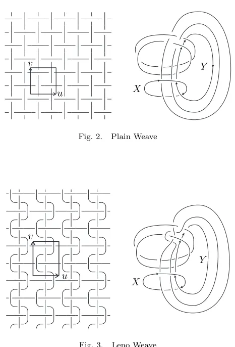
A schematic view of a fabric, with its face uppermost, and a kernel for it, are shown in Figure 1.
1.2. Some examples
L L L L
L L L L
L L L L
L
X
Y
Fig. 1. A kernel for a fabric
found in the books by Watson, [11,12], and Spencer, [14], and some of the primary structural elements are described in [13].
u v
X
Y
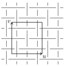
Fig. 2. Plain Weave
u v
X
[image:3.595.194.427.375.718.2]Y
u v
X
Y
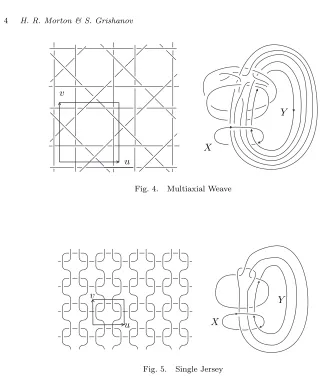
Fig. 4. Multiaxial Weave
u v
X
[image:4.595.118.438.131.507.2]Y
Fig. 5. Single Jersey
Different choices of repeating cell for a given fabric will give rise to different kernels. For example, choosing the cell shown in Figure 6 for the single jersey fabric gives the kernel shown.
u′
v′
X′
[image:4.595.177.430.597.701.2]Y′
1.3. Fabric kernels
The original fabric can be recovered from any one of its kernels. Since the region between the two auxiliary componentsX andY is topologically a thickened torus this means that the diagram on the torus can be recovered. The whole fabric can be reconstructed as a doubly periodic plane pattern by unwrapping the torus, - in effect constructing the inverse image of the diagram on the torus under the universal cover of the torus by the plane.
We adopt the namefabric kernel for such links.
Definition 1.1. Afabric kernelis a link consisting of two distinguished unknotted componentsX andY which form a Hopf link and one or more further components representing the fabric strands.
Any fabric kernel determines a fabric as above. Many fabric kernels will give rise to fabrics which decompose into disconnected layers or strips, or can prove physically difficult to make. The problem of identification of such structures which are not textiles from the traditional point of view is a part of a wider problem of enumer-ation of all possible textile structures. Some restricted subclasses corresponding to variants of traditional woven or knitted material will be of particular interest to us, but much of our theoretical work will apply to very general fabric links.
We show in the corollary to Theorem 3.3 how to use the classical multivariable Alexander polynomial of a fabric kernel to tell whether the resulting fabric contains any closed components. Suchchain mail type of fabric is impossible to make using traditional textile technology, and it is useful to be able to identify readily the corresponding fabric kernels.
In section 3.3 we show how to compare the polynomials for different kernels for the same fabric. TheAlexander data, which can be displayed as described in section 3.3 on a diagram of the fabric, can be found from any given kernel, and allows the polynomial of any other kernel to be readily calculated.
The Alexander data is then enough to allow comparison of different fabrics. While two different fabrics can give rise to the same Alexander data the size of the kernels must be sufficiently large for this to be possible, and an inventory of small fabric kernels using their polynomials will give a good means of listing the corresponding fabrics. We expect that more detailed comparisons of two fabrics will be best conducted by using kernels of approximately the same size - measured for example by the number of crossings in a repeating cell.
2. The axial type of a strand in a fabric
Suppose that we are given a fabric lying in a thickened plane, with a discrete group G of invariant translations generated by two independent elements u and v. We shall assume that the normal directionu×v lies to the face side of the fabric.
Any strand of yarn in the fabric is invariant under some subgroup of G. This subgroup is either trivial, when the strand is a closed curve, or is infinite cyclic, generated by some w ∈ G. The element w can be recognised, up to sign, as the smallest translation inGthat carries one point of the chosen strand to another point of the same strand. If the strand is oriented then we selectwso as to translate the strand in its preferred direction.
Definition 2.1. Theaxial type of a strand in a fabric is 0 if the strand is closed and is otherwise a generator w of the subgroup of translations which leaves the strand invariant.
Remark 2.2. Once we have chosen generatorsuand v forGeach axial type has the formw=αu+βv for some integers (α, β), determined up to an overall sign if the strand is unoriented.
For example, in the single jersey fabric shown in Figure 5 all fabric strands have axial typeu. In fact all strands are equivalent under translations inG, and yield a single fabric component in the kernel.
In general there may be two or more inequivalent strands with the same axial type. For example in Leno weave (Figure 3) there are two inequivalent strands with axial typeuand two with axial typev, while the multiaxial fabric in Figure 4 has strands of typeu, v, u+v andu−v.
2.1. Axial type and kernels
We can identify the axial type of the strands in a fabric by calculating certain linking numbers in a kernel for the fabric.
Assume that the kernel has been constructed using a choice of generators u, v for the group G of invariant translations. In the torus T2 = R2/G the lines in
the directions of uandv become closed curves,U and V say, which generate the homology groupH1(T2). A strand in the fabric with axial typew=αu+βv will
become a closed curveW in the thickened torusT2×I which representsαU+βV
in its homology group. Now the curves X and Y in the fabric kernel lie parallel to U and V respectively on either side of the standard thickened torus. They are oriented so that lk(X, U) = 0, lk(X, V) = 1, lk(Y, U) = 1, lk(Y, U) = 0. Since W = αU +βV in the homology of T2×I ∼= S3−(X ∪Y) we get lk(X, W) =
αlk(X, U) +βlk(X, V) =β and similarlylk(Y, W) =α.
biu+aiv, whereai=lk(X, Ti) and bi=lk(Y, Ti). In particular the strands in the fabric corresponding to Ti areclosed curves if and only ifai=bi = 0.
3. The multivariable Alexander polynomial For a linkL⊂S3withr >1 oriented componentsX
1∪. . .∪Xrthe groupH1(S3−L)
is free abelian of rankr. It has distinguished generatorsx1, . . . , xr represented by oriented meridians of the components. The multivariable Alexander polynomial ∆L is an element of the integer group ring Z[H1(S3−L)] and is thus a Laurent
polynomial in Z[x±11 , . . . , x±1r ]. It is defined up to a unit in this ring, and thus up to multiplication by a signed monomial±xa1
1 · · ·xarr.
With some care an absolute version of the polynomial can be defined, as in [7]. The Torres symmetry condition (3.1) shows that
∆L(x−11 , . . . , x−1r ) = (−1)rx1m1. . . xmrr∆L(x1, . . . , xr), for some integersm1, . . . , mr. Multiplying ∆Lby the monomialx
1 2m1
1 . . . x
1 2mr
r gives Murakami’s absolute version, up to sign, with the property that
∆L(x−11 , . . . , x−1r ) = (−1)r∆L(x1, . . . , xr). In this format we need to use half-integer powersx12
i of some of the variables{xi}. We make use of the absolute version in presenting the Alexander data, but for many of the properties and calculations it is enough to allow a monomial multiple, so as to avoid negative powers of the variables.
In the case of a single component link, in other words a knot K, we write ∆K ∈Z[t±1] for its classical Alexander polynomial, and in this paper we use the non-standard notation ∆K to denote the rational function ∆K = 1−1t∆K. In this way we can give formulae for the behaviour of the Alexander polynomials of related knots and links in a uniform way, without having to treat the single component case, r = 1, separately. The formulae can be most consistently handled in the context of Reidemeister torsion, where an excellent recent account is given in [10]. Here we give a summary of the properties needed, following the constructions of Fox and Torres based on Fox’s free differential calculus [9,1].
3.1. Deletion of components
For an oriented linkLwith componentsX1∪. . .∪Xrthe curveXi represents the monomialY
j6=i xlij
j as an element ofH1(S3−(L−Xi)), where lij =lk(Xi, Xj)∈Z is the linking number ofXi andXj. We write
< Xi>= Y
j6=i xlij
j (3.1)
Theorem 3.1 (Torres).
∆L|xi=1= (1−< Xi>)∆L−Xi.
Remark 3.2. If the componentXi has a non-zero linking number with at least
one of the other components then < Xi >6= 1. It is thus possible to recover the Alexander polynomial of the sublink L−Xi where Xi is removed, starting from the polynomial ∆L of the whole link, unlessXi has linking number 0 withall the other components ofL.
For the absolute versions of the invariants in Theorem 3.1 the factor < Xi>
1
2 −< X
i>−
1
2 appears in place of 1−< X
i>.
3.2. Closed components in a fabric
We start from a fabric kernelL. ThenL=X∪Y ∪T1∪. . .∪Tk, whereX and Y are the distinguished face and back curves forming a Hopf link. The complement ofX ∪Y forms a standard thickened torus containing the remaining components T1, . . . , Tk, termed the fabric components of L. These curves correspond to the strands of yarn in the fabric resulting from unwrappingL.
The curve Ti in the fabric kernel unwraps to give closed components in the covering fabric if and only if it has linking number 0 with both of the auxiliary curvesX andY.
Theorem 3.3. LetL=X∪Y∪T1∪. . .∪Tkbe a fabric kernel. Writeai=lk(Ti, X)
andbi=lk(Ti, Y). Then its Alexander polynomial ∆L(x, y, t1, . . . , tk)satisfies ∆L(x, y,1, . . . ,1) =
k Y
i=1
(1−xaiybi)∈Z[x±1, y±1].
Proof. After setting alltj= 1 we have< Ti>=xaiybiby equation (3.1). Repeated use of theorem 3.1, suppressing the componentsT1, . . . , Tk in turn, gives
∆L(x, y,1, . . . ,1) = k Y
i=1
(1−xaiybi)∆
X∪Y.
Since the remaining linkX∪Y is the Hopf link, whose Alexander polynomial is 1, the result follows.
Corollary 3.4. There is a closed component in the covering fabric ofLif and only if∆L(x, y,1, . . . ,1) = 0.
Proof. The Laurent polynomialQk
i=1(1−xaiybi) is equal to 0 in Z[x±1, y±1] if
and only ifai=bi= 0 for somei.
Remark 3.5. The element< Ti>=xaiybi represents the homology class ofTi in the thickened torus S3−(X ∪Y). Written additively this is b
and V are determined by the generatorsu and v as in subsection 2.1. The axial typebiu+aiv of the corresponding strands in the fabric, and indeed the number of inequivalent strands of each axial type, can then be read off immediately from ∆L, so long as there are no closed strands in the fabric.
To determine the axial types using Theorem 3.3 it is enough to be given the polynomial ∆Las a function ofx, yandtonly, where all the fabric variablestihave been set equal to t. If there are no closed components in the fabric we can then recover the numberkof fabric components in the kernel, and the axial types of the corresponding fabric strands, from the factors in the evaluation with t= 1.
In a traditional woven fabric there are just two axial types, corresponding to the warp and weft directions, while a traditional knitted fabric has only one type.
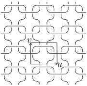
[image:9.595.243.378.380.491.2]More sophisticated woven fabrics with multiaxial types have recently been in-troduced, [15], such as the fabrics shown in Figure 4 and 15. Knitted fabrics too may have warp and weft type inserts, as in Figure 7, leading to a multiaxial fabric.
Fig. 7. Single Jersey with warp and weft inlays
From this basic analysis of the polynomial of a kernel we can identify immedi-ately the axial types, although a detailed discussion of whether a fabric is woven or knitted in the appropriate sense may not be available from the polynomial alone. Of course if the kernel has more than two different axial types then we can cer-tainly conclude that the fabric is not a traditional woven structure, while equally a traditional knitted structure can be excluded unless there is a single axial type.
We give here the polynomials for the kernels of several fabrics. Example 3.6.
Single jersey with a closed thread around the fabric thread
∆L= (tx−t−x)(t+x−1)(t−1)(y−1). Example 3.7.
∆L = (tx−t−x)(t+x−1)(t2−t+ 1)(y−1). Example 3.8. Single jersey with warp and weft inlays, as in Figure 7:
∆L= (t+x−1)(tx−t−x)(px−1)(ey−1)(y−1),
where the jersey strand has variablet, the warp strand has variableeand the weft has variablep.
Example 3.9.
The Alexander polynomial for the kernel of the chain mail pattern shown in Figure 8 is
∆L= (x−y)(1−xy)(1−t). (3.2)
u v
Fig. 8. Chain Mail
This is one of the fabric kernels which, like Example 3.6, does not correspond to a physically constructible textile fabric, on account of the closed components. The substitutiont= 1 for the fabric variables leads to the value 0, as required by Theorem 3.3.
3.3. The Alexander data for a fabric
We now present a normalised form of the Alexander polynomial of a kernel giving rise to an array of polynomials in the fabric variables which are independent of the choice of generatorsuandv. The result is a set of invariants for the fabric which readily determine the Alexander polynomial forany choice of kernel.
Start from the Alexander polynomial ∆L(x, y, t1, . . . , tk) of a kernel L deter-mined by a choice of generatorsuandv of the group of translations of the fabric.
Writeti=s2i and set
U =yYsai
i , V =x Y
sbi
i (3.3)
ualgebraicallyai times in the direction ofvand crosses the edgevalgebraicallybi times in the direction ofu.
TheAlexander dataof the fabric consists of the coefficients of ∆Lwhen written as a polynomial in U andV. When written in this way we say that the Alexander polynomial ∆L is indata form.
The Alexander data coefficients are Laurent polynomials in the fabric variables {si}. In Theorem 3.10 we show how they depend essentially on the fabric only and not on the choice of kernel.
Write
∆L= X
Lα,βUαVβ
and setTw=Lα,β for eachw=αu+βv∈G. In this way we associate a Laurent polynomialTw(s1, . . . , sk) to each elementwin the translation groupG.
Since the Alexander polynomial ∆Lis often defined only up to multiplication by a signed monomial inx, y, t1, . . . , tkthere is a measure of ambiguity in the definition of Tw. Apart from this ambiguity, which can be eliminated up to an overall sign by use of the Torres symmetry conditions, the elementsTware independent on the choice of kernel, and are termed collectively theAlexander data of the fabric. The independence is made precise in the following invariance theorem.
Theorem 3.10. The Alexander data of a fabric is independent of the choice of generators for G, up to an overall multiplication by a monomial in s1, . . . , sk and
translation by an element ofG. When we use generatorsu′andv′ in place ofuand
v to form a kernelL′, then the resulting polynomialsT′
w, w∈Gsatisfy the equation
Tw′ =±mTw+g,
for someg∈Gand monomial min s1, . . . , sk independent of w.
Proof. Our choice u, v of generators for the group of translations G determines the repeating cell used to construct the kernel. Lines in the plane in the directions of uandv become closed curves U and V in the quotient torusT2 =R2/G. The
face torus is embedded as the boundary of a neighbourhood of the face curve X and the back torus as the boundary of a neighbourhood of the back curveY, where X andY are parallel to the closed curvesU andV respectively. In this embedding the face torus contains curvesmX andlX, which are respectively the meridian and longitude of the curve X. The back torus correspondingly contains mY and lY, giving the longitude and meridian curves as lX = U × {1}, lY =V × {0}, while mX =V × {1}andmY =U× {0}.
In terms of the generatorsx, y, t1, . . . , tk for the homologyH1(S3−L) we have
U × {0}=y, U× {1}=< X >=yYtai
i ,
V × {1}=x, V × {0}=< Y >=xYtbi
whereai=lk(Ti, X) andbi=lk(Ti, Y). The variablesU =yQsaii andV =x Qsbi
i introduced in equation (3.3) thus represent an ‘average’ of the homology of the curves U and V on the front and back faces of the torus. When the homology H1(S3−L) is written additively we have
2U =U× {0}+U× {1} 2V =V × {0}+V × {1}.
A different choice of generatorsu′, v′forGgives rise to a different repeating cell,
and a different kernel for the fabric. Now the complement of a kernel inS3 is the
complement of the fabric quotient in the thickened torusT2×I. This complement
is unchanged by the new choice of generators forG, so thatS3−L′∼=S3−L. What doeschange is the curves on the face and back tori that correspond to the longitudes and meridians of the face and back curves in the two kernels. We then know that ∆′
L= ∆L, when the variables are changed appropriately. We need to compare the elementsx, y, t1, . . . , tkandx′, y′, t1, . . . , tkas elements ofH1(S3−L) =H1(S3−L′).
The comparison is very straightforward when we use the data form of the two polynomials.
Lemma 3.11. We can suppose that
u′=pu+qv, v′ =ru+sv
withp, q, r, s∈Zandps−qr= 1. Then
U′=pU+qV, V′ =rU +sV,
when written additively as elements ofH1(S3−L).
Proof. The curvesU′, V′ onT2=R2/Gcorresponding to the vectorsu′, v′satisfy
the equations
U′=pU+qV, V′=rU+sV,
as elements ofH1(T2).
Hence on the boundary of the thickened torus we have
U′× {i}=pU× {i}+qV × {i}, V′× {i}=rU× {i}+sV × {i}, fori= 0,1.
Adding these equations fori= 0 and i= 1 inH1(S3−L) we then have
2U′ = 2(pU+qV),2V′= 2(rU+sV).
The multivariable Alexander polynomial ∆Lof a fabric kernelL=X∪Y∪T1∪
. . .∪Tkis an element of the integer group ringZ[H1(S3−L)], and hence is a Laurent
quotient in the thickened torusT2×I. Hence if L′ is another kernel for the same
fabric it will have the same Alexander polynomial, sinceπ1(S3−L′) =π1(S3−L),
written now in terms of different generators of the groupH1(S3−L).
In terms of the Alexander polynomial we can relate ∆L′to ∆L, up to multiplica-tion by a signed monomial, using the multiplicative versionU′=UpVq,V′ =UrVs of Lemma 3.11.
The Alexander data polynomialsT′
wdefined using the kernelL′ are given by the equation ∆L′ =PTw′(U′)α
′ (V′)β′
, wherew=α′u′+β′v′. Making the substitution
forU′ andV′ gives
∆L = ∆L′ = X
Tw′U(α ′p+β′r)
V(α′q+β′s)=XTw′UαVβ,
with α=α′p+β′r, β =α′q+β′s. Hence, in terms of the Alexander data defined
usingLwe haveT′
w=Tg withg=αu+βv. Nowg= (α′p+β′r)u+ (α′q+β′s)v= α′u′ +β′v′ = w, giving the invariance result that T′
w = Tw, up to the overall ambiguity of the definition of the Alexander polynomial.
3.4. Changing the choice of the repeating cell
Given the Alexander data of a fabric, calculated using any one choice of generators for the translation group, Theorem 3.10 shows how the multivariable Alexander polynomial for any other kernel of the same fabric can be found.
We can now compare the Alexander data from two fabrics quite readily. We just need one choice of unit cell for each to provide the Alexander data. Having put the two sets of data onto a plane we can see that if the fabrics themselves are affinely equivalent, in other words related by a translation and a linear transformation, then one set of data will transform to the other by a similar affine transformationϕ carrying the coefficient polynomials{Tw}for one fabric to the polynomials{Tϕ(w)}
of the other. Fabrics with inequivalent Alexander data are then inequivalent. In particular the number and affine location of the non-zero polynomials in the Alexander data is a simple invariant of the fabric. This could be refined, without presenting the whole data, to include the degrees of each fabric variable at the plane locations.
3.5. Presenting the Alexander data
Superimpose a grid on the fabric by choosing a pointOas origin in the plane, and label the translates of O by elements of the group G. At the translate of O by w ∈ G place the polynomialTw. This display of the polynomials Tw is uniquely determined by the choice of origin, where the polynomials themselves have been normalised, up to an overall sign, by multiplying all polynomials by a monomial in the variables{si=t
1 2
i} so as to respect the Torres symmetry conditions.
Thus to find the Alexander data polynomials Tw we choose any kernelL and put ∆L into data form by setting x=V /Qsbii and y =U/
Q sai
Conversely, given uand v we can recover the data form of ∆L in terms of U andV immediately from the Alexander data. Equation (3.3), using the numbersai andbi calculated from the choice ofuandv, then gives ∆L in terms ofxandy. Example 3.12.
We may compare the single jersey data derived from the different choices of unit cell shown in Figures 5 and 6.
From a braid presentation of the single jersey kernel L shown in Figure 5 we can calculate its multivariable Alexander polynomial
∆L= (1−y)(1−x−t)(x+t−tx),
where the variable t = s2 is the single fabric variable. Setting t = 1 gives y−1
up to monomial multiples, confirming that the fabric has a single axial directionu. From the intersections with the cell edges we have the Alexander data substitution U =yandV =xs.
A similar braid based calculation for the polynomial ∆L′ of the kernel in Figure 6 gives
∆L′ = (1−y′)(x′−tx′+ty′)(x′−y′+ty′)
up to a signed monomial multiple. Again the intersections with the cell edges show that the data substitution is U′ = y′, V′ = x′s. Now this kernel is related to L
by the choice of generators u′ = u, v′ = u+v. Consequently the substitution
U′=U, V′ =U V will convert the data form forL′ into the data form forL, up to
a monomial multiple.
We can exhibit the Alexander data starting from either data form. On the one hand we have
∆L= (1−U)(1−s2−V /s)(s2+ (s−1−s)V), while
∆L′ = (1−U′)((s−1−s)V′+s2U′)(V′/s−(1−s2)U′) =U2∆L after the substitution.
Multiplication bys−1 gives the Torres symmetric form of the data displayed in
matrix form below.
s−3−s−1 s−1−s−3
−s2+ 3−s−2s2−3 +s−2
s3−s s−s3
Here and in the examples below we present the Alexander data as a matrix of polynomials based on the stated choice of u and v. The rows of the matrix correspond to translations by multiples ofu, read from left to right, and the columns to multiples ofv, read from the bottom up.
Example 3.13.
In the previous example we have used the single jersey fabric viewed from its traditional face side. When viewed from the back, as in Figure 10, the polynomial for the kernel is ∆L= (1−y)(t2x−tx+ 1)(t2x−t+ 1). This gives the normalised
[image:15.595.266.356.303.392.2]u v
Fig. 10. Single Jersey, from the back
Alexander data shown in Figure 11.
s3−s s−s3
−s2+ 3−s−2s2−3 +s−2
s−3−s−1 s−1−s−3
Fig. 11. Single Jersey (back) data
Example 3.14. The Alexander polynomial for the kernelL of plain weave corre-sponding to the choices ofuandvin Figure 2 is
∆L =−1 + 2px+ 2ey−p2x2−e2y2+ ((1−e)2(1−p)2−4ep)xy +2p2ex2y+ 2pe2xy2−e2p2x2y2,
where the two fabric strands in the direction ofuhave the meridian variablepand those in the direction v have variable e. Write e = a2 and p =b2. Then setting
U =y/a2 = y/e and V =x/b2 =x/p, as required by equation (3.10), gives the
data form
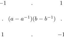
[image:15.595.251.369.470.534.2]This leads to the data shown in Figure 12.
−1 2 −1
2 (a−a−1)2(b−b−1)2−4 2
−1 2 −1
Fig. 12. Plain Weave data
Example 3.15.
Leno weave, which was presented in Figure 3, has four threads in the minimal unit cell; two non-equivalent threads are running in theudirection and two in the vdirection.
The Alexander data for Leno weave is presented in Figure 13, where P = (a−2−1 +a2)(b−1−b)2+ 2
Q= 2(a−1−a)2(b−1−b)2+ 2(a−2−a2)2−(a−2b−1+a2b)2+ 2.
−1 2 −1 P Q P
−1 2 −1
Fig. 13. Leno weave data
Example 3.16. The Alexander data for chain mail is shown in Figure 14. It is based on the choice of generators in Figure 8, and the corresponding Alexander polynomial in equation (3.2). In this case the data form is given simply byU = y, V =x.
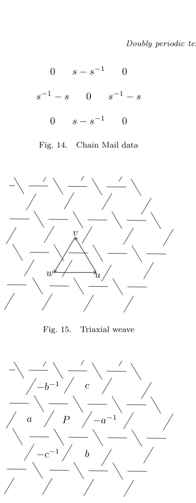
Example 3.17. The triaxial weave shown in Figure 15 has a lattice of symmetries with a 3-fold symmetry when the strings are oriented in the three axial directions, u,v andw=−u−v as shown.
0 s−s−1 0
[image:17.595.224.416.109.602.2]s−1−s 0 s−1−s 0 s−s−1 0 Fig. 14. Chain Mail data
u v
w
Fig. 15. Triaxial weave
a
b c
−a−1
−b−1
−c−1 P
Fig. 16. Triaxial weave data
3.6. Multiple repeating cells
For comparison purposes it can be useful to look not just at a minimal area repeat of a pattern in a fabric. This means that we use a repeating cell whose edges are determined by two vectors u′, v′ in the group G of translations which generate a
proper subgroup ofG. It is always possible to choose generatorsu, vforGandu′, v′
can insist further thatu′ =suandv′ =rv where ris a multiple ofs. Then every
vectorw′ inH is a multiplew′=swof a vectorwinG, and in many cases we will
haves= 1.
The relation between the Alexander data for the fabric using the full groupG, corresponding to a minimal choice of repeating cell, and the data derived from using the translations inH only (and thus only considering a larger repeating area) can be determined by comparing the Alexander polynomials of the kernelsLand L(r)
which come from the choice of translationsu, vandu, w=rv respectively. These polynomials are related by a more general result of Salkeld [8] connecting the multivariable polynomials for a linkLwith a distinguished unknotted compo-nentX and the linkL(r)given by taking ther-fold cyclic cover ofLbranched over
X. The two kernels above are related in this way, so Salkeld’s result applies. There is an r-fold covering map p from the complement of L(r) to the
com-plement of L, inducing a map p∗ on the first homology group. Salkeld’s theorem
expressesp∗(∆L(r)) in terms of ∆L as follows.
Theorem 3.18 (Salkeld). Writexfor the meridian variable corresponding to the componentX inL. Then
p∗(∆L(r)) =
Y
∆L(ζx),
asζ runs through allrth roots of1.
Corollary 3.19.
The data form of∆L(r), in terms ofU andW, corresponding to the translations
uandw=rv, satisfies the equation
p∗(∆L(r)) =
Y
∆L(ζV),
asζ runs through allrth roots of1, whereW =Vr.
Proof. In the data form for ∆L we have V = xQsaii, while in ∆L(r) we have
W =X(Qsai
i )r, and p∗(X) =xr. Now ∆L(ζx), given by replacingxwithζx, can be found from the data form by replacingV withζV.
Salkeld’s theorem does not give the complete polynomial for the covering link, in the case when there is more than one component ofL(r)covering some component
ofL, sincep∗(∆L(r)) has the same variable for all components which project to the
same component in L. In the case of fabric kernels we would expect to make this restriction in any case, as the different components of L(r) with the same image
must be equivalent strands in the fabric under the full groupGof translations. We would only use a different variable if they were to be considered different in the fabric, and in this case a translation carrying one to the other would not be part of the groupG. The meridian for the branch curve inL(r)projects toxrin L, and so the polynomial ∆L(r), with equivalent components in the fabric having the same
one factor, corresponding to the root ζ = 1, when the branch curve meridian is replaced byxr.
If ∆L factorises, then ∆L(r) can be found as a product using the same
opera-tion on each factor. Indeed the operaopera-tion of passing from ∆L to p∗(∆L(r)) can be
regarded formally as replacing the roots (for x) of ∆L by their r-th powers; the coefficients of powers ofxinp∗(∆L(r)) are integer polynomials in the coefficients of
∆L.
Example 3.20. We can find the data form of the Alexander polynomial for single jersey doubled horizontally, using the cell with sides w= 2uandv in terms of the generatorsuandv shown in Figure 5 for the translation group. This is given from Salkeld’s theorem by taking the 2-fold cover of the kernel branched over the curve Y. The result, as a polynomial in W and V, will be the polynomialP(W, V, t) = ∆L(U, V, t)∆L(−U, V, t) withW =U2. Using the data form ∆L= (1−U)(1−s2− V /s)(s2+ (s−1−s)V) we get
P = (1−U)(1 +U)(1−s2−V /s)2(s2+ (s−1−s)V)2 = (1−W)(1−s2−V /s)2(s2+ (s−1−s)V)2.
The polynomialQfor single jersey doubled vertically, corresponding to uand w = 2v has Q(U, W, t) = ∆L(U, V, t)∆L(U,−V, t) with W =V2, giving the data form
Q= (1−U)2((1−t)2−W/t)(t2−(1−t)2W/t),
where both fabric strands have the variablet. This converts to the Alexander poly-nomial by settingU =y, W =xs2=xt, to get
Q= (1−y)2((1−t)2−x)(t2−(1−t)2x).
A more refined version of the Alexander polynomial, using different variables for the two strands, can be calculated directly from a kernel as
(1−y)2((1−t1)(1−t2)−x)(t1t2−(1−t1)(1−t2)x).
Example 3.21. The Alexander polynomial for 1×1 rib, which alternates face and back loops in theudirection, is
∆L= (tx−t−x)(t+x−1)(t2x−tx+ 1)(t2x−t+ 1)(y−1).
This polynomial is a mix of the polynomials for the face and back kernels of single jersey, and can be compared with the multiple cell case of single jersey in the previous example, where two face loops are repeated in theu direction. This was calculated above to be
∆L= (tx−t−x)2(t+x−1)2(y−1). A repeat of the back loop in theudirection gives
These two polynomials are inequivalent to the polynomial for 1×1 rib.
Here we use the terms ‘face loop’ and ‘back loop’ for the basic units in single jersey when seen from the front or back of the fabric, as in Figures 5 and 10 respectively.
For the general case ofm×nrib, which is a combination ofm≥0 face andn≥0 back loops in theudirection, we have
∆L= ((tx−t−x)(t+x−1))m((t2x−tx+ 1)(t2x−t+ 1))n(y−1). Indeed this polynomial is the same irrespective of the order in which the face and back loops occur, so that the standard 2×2 rib gives the same data as the 1×1 rib repeated twice in theudirection. We have tried comparing the polynomials in which alternate rows have variablest1andt2, to see if this is enough to distinguish
these fabrics, but again the results are the same. Example 3.22.
Alternate knit and purl rows, sometimes known asgarter stitch. This is a combina-tion of one face and one back loop in thevdirection, and has Alexander polynomial
∆L= (1 + (1−t1)(1−t2)x)((1−t1)(1−t2) +t1t2x)(y−1)2.
It can be compared with the polynomial for plain knit or purl fabric, calculated with different variablest1 andt2 for alternate rows.
For two face loops in thev direction the polynomial is
∆L= (t1t2−(1−t1)(1−t2)x)((1−t1)(1−t2)−x)(y−1)2.
For two back loops in thev direction the polynomial is
∆L= (t21t22x−t1t2+t1+t2−1)(t21t22x−t21t2x−t22t1x+t1t2x−1)(y−1)2.
Replacing xby 1/t1t2xconverts the purl to the plain version here, and leaves
the polynomial of the mixed fabric unchanged. It is possible to use the different signs in the brackets to distinguish the mixed fabric with alternately knit and purl rows from the plain fabric viewed from either side, by settingt1=t2=−1.
Example 3.23. We can use Salkeld’s theorem as in Example 3.20 to calculate the polynomials for plain weave when doubled in either theuor the v directions. We start from the data form of the polynomial ∆L(U, V, e, p) given in Example 12, and in each case repeat the same variablepfor all the weft strands (in theudirection), and efor all the warp strands (in the v direction), to arrive at a formula for the multiple cell polynomial.
Here
∆L=−(1−U)2(1 +V2) + [2 + (1−e)2(1−p)2U/ep+ 2U2]V, giving
Q= (1−U)4(1 +W)2−[2 + (1−e)2(1−p)2U/ep+ 2U2]2W.
The Alexander data can be presented on a translation lattice on the fabric, after expansion in terms of U and W. The Salkeld factorisation characteristic of the multiple cell repeat is not immediately obvious in the lattice, but shows up from the Alexander polynomial when the variableW is replaced byV2.
In fact the plain weave itself as given traditionally is invariant under a larger group of translations than those generated byuandv. The translations by 1
2(u+v)
and 12(u−v) generate the full group of invariant translations, and give rise to half-size repeating cells. The kernel based on the choice ofu, v′ =1
2(u+v) can be used
to calculate the Alexander data for this larger group of translations. If we use the translations 1
2uand 1
2vto index rows and columns of a matrix then the Alexander
data has the simple form shown, where as before we writee=a2 andp=b2.
−1 . 1
. (a−a−1)(b−b−1) .
[image:21.595.257.365.453.522.2]1 . −1
Fig. 17. Plain Weave minimal cell data
In this matrix view of the Alexander data the entries indicated by a dot (.) cor-respond to translations which do not belong to the group. The Salkeld factorisation of the traditional polynomial arising from the fact that the repeat lattice is not minimal can be seen from its data form in terms ofU andV by puttingU V =V′2.
Example 3.24. We can also see examples of the multiple cell repeat when we study twills. Figure 18 shows a picture of a 1/2 twill, with the traditional repeating cell based on vectorsuand v.
The complete translation symmetry group is generated byuandv′ =1
3(u+v),
giving a repeat cell of one third the size, shown in Figure 19.
The data for the kernel based onuandv′is given here, withudrawn horizontally
u v
Fig. 18. 1/2 twill in traditional representation
[image:22.595.225.380.467.553.2]u w
Fig. 19. Minimal unit cell of 1/2 twill
√
ab −p
b/a 0
0 p
b/a(a−1−a)(b−1−b) 0
0 p
a/b(a−1−a)(b−1−b) 0
0 −p
a/b 1/√ab
When placed on the plane of the fabric the data, drawn with 13uhorizontally and 1
3v vertically, appears as shown in Figure 20.
√
ab . . −p
b/a
. . p
b/a(a−1−a)(b−1−b)
. p
a/b(a−1−a)(b−1−b) . .
−p
[image:22.595.160.448.611.700.2]a/b . . 1/√ab
In this array a dot (.) is again used for entries which do not correspond to any translation symmetry, as in the minimal cell display for plain weave shown in Figure 17.
As in the case of the minimal cell repeat for plain weave, discussed above, Salkeld’s theorem shows that the data form of the Alexander polynomial for the kernel based on uand v will factorise when we writeU V =V′3, corresponding to
the relation u+v= 3v′. One of the resulting factors, when written in terms ofU
andV′, gives the data form for the minimal cell based onuandv′. A direct check
starting from the Alexander polynomial of the kernel based onuandvdoes indeed confirm this.
More generally, an m/n twill consists of a weave in which there are m warp overlaps andnweft overlaps on any warp or weft thread within the repeat, with an offset of one thread in each successive row. Takeuandvas horizontal and vertical translations bym+nthreads. These are in the symmetry group of the fabric, but the complete symmetry group can be generated byuandv′= 1
m+n(u+v), giving a minimal repeat cell of 1
m+n times the obvious cell generated byuand v. Plain weave itself can be regarded in this context as a 1/1 twill.
3.7. Layered fabrics
If a fabric decomposes into two separate layers then the plane separating the two lay-ers becomes a torus separating a kernelNfor the fabric into some curvesW1, . . . , Wr on one side of the thickened torus, coming from the lower layer of the fabric, and others T1, . . . , Tk on the other side coming from the top layer. The face curve X lies on the side of the torus containing the curvesT, while the back curveY lies on the side containing the curvesW. Because of the torus separating the components ofN there is a decomposition of the polynomial ∆N as a product. This arises as a special case of a general result of Fox, best described in the following ‘Fox gluing formula’.
Suppose that we have two linksL=T1∪. . .∪Tk∪AandM =W1∪. . .∪Wr∪B. Remove a neighbourhood VA of A and VB of B and glue S3−VA to S3−VB, matching the meridianaofVA to the longitude ofVB and the meridianbofVB to the longitude ofVA. The curvesT1∪. . .∪Tk∪W1∪. . .∪Wr form a linkN in the resulting manifold, which is againS3if one ofA orB is unknotted.
Theorem 3.25 (Fox gluing formula). ([1]) The Alexander polynomial of the linkN resulting from this gluing is given by
∆N = ∆L∆M
after substituting a=< B >in Z[w±1j ]andb=< A >in Z[t±1i ].
Remark 3.26. Theorem 3.1 is a corollary of this formula. Take the linkM to be the unknotB with no further components. Then< B >= 1 and ∆M =
linkNis the linkL−A, and Theorem 3.25 shows that (1−< A >)∆L−A= ∆L|a=1.
Theorem 3.27. If a fabric kernel N arises from a layered fabric as above, then its Alexander polynomial factorises as
∆N = ∆L(xL, yM Y
waj
j , t1, . . . , tk)∆M(xL Y
tbi
i , yM, w1, . . . , wr),
where the numbersaj are the linking numbers of the fabric strands in the bottom
layer with the face curve, while the numbersbjare the linking numbers of the strands
in the top layer with the back curve.
Proof. If a fabric kernel N arises from a layered fabric then N comes from a gluing construction to which Theorem 3.25 applies. Define two other links which correspond to the two layers of the fabric. These are the kernel for the top layer, L=XL∪YL∪T1∪. . .∪Tk, given by deleting the curvesW fromN, and the kernel for the bottom layer,M =XM∪YM∪W1∪. . .∪Wr, given by deleting the curvesT. Then the linkN comes fromLandM by the gluing construction, takingA=YL andB=XM.
Now < YL >=xLQtbii and < XM >=yMQwjaj. In N the auxiliary curves areX =XL, the face curve of the top layer, andY =YM, the back curve of the bottom layer. Hence the Alexander polynomial factorises as
∆N = ∆L(xL, yM Y
waj
j , t1, . . . , tk)∆M(xL Y
tbi
i , yM, w1, . . . , wr).
Assuming that the fabric has no closed components this factorisation is non-trivial, since evaluation of either factor when ti = wj = 1 for alli and j gives a polynomial which is not 0 or 1.
Corollary 3.28. If a fabric decomposes into r layers then the polynomial of any kernel factorises intor factors corresponding to the kernels of the layers.
The number of non-trivial factors in the Alexander polynomial of any kernel is then an upper bound for the number of layers. It follows that if the polynomial ∆N does not factorise then the fabric does not decompose into layers.
The converse does not hold, since some fabrics which do not decompose into layers can have kernels whose polynomials do factorise non-trivially.
3.8. Strip-like fabrics
fabric if its polynomial has no factor of 1−y, or has a non-trivial dependence on x. The knitted fabrics studied in examples 3.12, 3.13, 3.20, 3.21 and 3.22, with u as their axial type, do indeed exhibit a factor 1−y, but the polynomials depend non-trivially on x, confirming that the fabrics do not fall into strips.
The warp-knitted chain illustrated in Figure 21 shows a linear chain repeated so as to give a doubly periodic fabric, in this case presented with a single axial type v . The Alexander polynomial of its kernel,
(x−1)(xt+ 1−t)(xt−x+ 1),
depends on xandt only, and has a factor of 1−x, both of which are pointers to the strip-like nature of the fabric. Its data form then depends on V only and the data appears as a linear array of polynomials in thev direction.
[image:25.595.246.377.362.477.2]u v
Fig. 21. Warp-knitted chain
An example of a fabric which is not a traditional knit or weave is the fishing net, shown in Figure 22. It has one axial type,u+v, relative to the choice of generating translations indicated, but it does not have the geometric characteristics of a knitted fabric with this as the thread direction.
u v
[image:25.595.258.363.597.702.2]The Alexander polynomial of the fishing net kernel based on this choice of generators is
t2x−t3x+t2y−t3y−4t3xy+ 2t2xy−txy−t5xy+ 3t4xy+t4−2t3+ 4t2−3t+ 1.
To convert to data form we set U = ys, V = xs, with t =s2. This leads to the
display of Alexander data,
s−1−s −s4+ 3s2−4 + 2s−2−s−4
s4−2s2+ 4−3s−2+s−4 s−1−s,
confirming that this is not a strip-like fabric.
3.9. Vassiliev invariants
In a recent paper, [3], Grishanov, Meshkov and Vassiliev have looked at the use of Vassiliev invariants of a curve in the thickened torus or Klein bottle as a tool for distinguishing textile patterns.
Following the paper of [5] in relation to Fiedler’s invariant we believe that the Alexander polynomial of a kernel can be used to find some of the Vassiliev invariants for a fabric with a single fabric curve.
Suppose that a kernelLhas been constructed from the fabric, with polynomial ∆L(x, y, t), normalised to have Torres symmetry. Expand ∆L(x, y, eh) as a power seriesPa
r(x, y)hr. The coefficients can be regarded as elements of the integer group ring ofH1(T2), wherexandyare represented by the curvesV andU respectively in
the torusT2. In this setting the polynomiala
rappears to be a Vassiliev invariant of degreerin the sense of [3]. The constant terma0is, by Theorem 3.3, the polynomial
1−xayb up to normalisation, and the termxayb represents the homotopy class of the fabric component. This is constant over all homotopic curves in the torus, as for the degree 0 invariant of [3].
The invariants of the fabric curve of degree 1 should also arise in this way. A check on the examples above with only one fabric component give the following results fora1.
Chain mail a0= 0 a1=x+x−1−y−y−1
Single jersey (face) a0= 1−y a1=a0(x−1−x)
Single jersey (back) a0= 1−y a1=a0(x−x−1)
m×nrib a0= 1−y a1=a0(n−m)(x−x−1)
Fish net a0= 1−xy a1= 12−x−y+12xy
Warp knitted chain a0= 1−x a1=a0(x+ 1−x−1)
4. Further investigations
similar program to handle links presented as plats, or even just from the diagram of the fabric inside a unit cell. This approach looks likely to relate to a presentation of the diagram on the torus as a genus 1 virtual knot, [4].
Acknowledgments
We would like to thank De Montfort University and the Mathematics and Modelling Research Centre at the University of Liverpool for support during this work.
References
[1] Fox, R.H. Free differential calculus.V. The Alexander matrices re-examined.Ann. of
Math. (2)71(1960), 408–422.
[2] Grishanov, S.A., Meshkov, V.R. and Omel′chenko, A.V. Kauffman-type polynomial
invariants for doubly periodic structures.J. Knot Theory Ramif.16 (2007), 779–788.
[3] Grishanov, S.A., Meshkov, V.R. and Vassiliev, V. Recognizing textile structures by finite type knot invariants. (Preprint, De Montfort University, 2008).
[4] Kauffman, L.H. and Manturov, V.O. Virtual knots and links.Tr. Mat. Inst. Steklova
252(2006), Geom. Topol., Diskret. Geom. i Teor. Mnozh., 114–133; translation in
Proc. Steklov Inst. Math.2006, no. 1 (252), 104–121.
[5] Morton, H.R. The Burau matrix and Fiedler’s invariant for a closed braid.Topology
and its Applications 95(1999), 251–256.
[6] Morton, H.R. The multivariable Alexander polynomial for a closed braid.
Low-dimensional topology (Funchal, 1998), 167–172,Contemp. Math.233, (Amer. Math.
Soc., Providence, RI, 1999).
[7] Murakami, H. A weight system derived from the multivariable Conway potential
function. J. London Math. Soc.59(1999), 698–714.
[8] Salkeld, J.O. Generalized exchangeable braids. PhD thesis, University of Liverpool, (1997).
[9] Torres, G. On the Alexander polynomial.Ann. of Math. (2)57(1953), 57–89
[10] Turaev, V.G. Torsions of 3-dimensional manifolds. Progress in Mathematics, 208.
Birkh¨auser Verlag, Basel, (2002).
[11] Watson, W. Advanced textile design. 3rd ed. ( Longmans, Green and Co., London, 1996).
[12] Watson, W. Textile design and colour. 3rd ed. ( Longmans, Green and Co., London, 1996).
[13] Emery, I. The primary structures of fabrics: an illustrated classification. (Thames and Hudson, London, 1994).
[14] Spencer, D.J. Knitting technology: a comprehensive handbook and practical guide. 3rd ed. (Woodhead Publishing, Cambridge, 2001).
[15] Dow, N.F. and Tranfield, G. Preliminary investigations of feasibility of weaving