Functional, Clustered, Feedforward, and Mesoscale Brain Networks

(1)

networks

Thesis by

Yazan N. Billeh

In Partial Fulfillment of the Requirements for the Degree of

Doctor of Philosophy

California Institute of Technology Pasadena, California

2016

(2)

c

(3)

c

(4)

To my family

(5)

Acknowledgements

This PhD would not have been possible without the support of the incredible team of individuals mentioned here.

First, I am extremely thankful to my advisor, Christof Koch, who agreed to supervise me even though he was moving to Seattle at the end of my first year. Instead of simply telling me to join another lab, he decided to mentor and foster my scientific abilities and I am profoundly grateful to him. I am humbled to say that not a single email went unanswered! It is remarkable how Christof was always supportive on an academic and personal level (such as when I needed knee surgery). An amazing mentor. Many thanks Christof.

Second, I am indebted and very thankful for the support and help of Markus Meister. He provided me with much more than desk space by allowing me to feel like a member of his lab at Caltech. I was able to be a part of the intellectual environment he creates by attending and presenting in group meetings and journal clubs and his door was always open to me to ask for suggestions and help. Simply put, I could not have done it without Markus. A key person who ignited the journey of my PhD is Costas Anastassiou. He was instru-mental in my learning by taking me under his wing and showing me the ropes of compu-tational neuroscience and Caltech. He was one of the reasons I came to Caltech and it has been a privilege to work with him. I looked forward to growing this strong relationship we formed.

I was also very fortunate to have collaborated with some brilliant scientists and I would like to acknowledge and thank Michael Schaub and Mauricio Barahona. Michael visited Caltech, from Imperial College London, for one month during my second year and we have been collaborating ever since. It is truly a pleasure to work with Michael and I know there is still more science and discoveries in our future. From Mauricio, I learnt a great deal about how to design, analyze, and present science. Thank you both.

(6)

which I am very grateful.

Moreover, I was lucky to work with exceptional scientists at the University of Wisconsin. It was a great learning experience for me and their support and time spent are highly appreciated. Thank you to Chiara Cirelli, Giulio Tononi, Alex Rodriguez, and the members of the Center for Sleep and Consciousness.

There are many people who must be acknowledged, and although briefly mentioned here they know how important and vital they were throughout my studies. I am grateful to all members of the Koch lab for all the support, adventures, and laughs during my time at Caltech. I also am thankful to the members of the Meister lab. In addition, friends from my time at Pasadena, Michigan, London, and Amman were part of the supportive team, allowing me to write this thesis, and to all of you I am deeply thankful.

Further, I would like to acknowledge and thank my committee for support throughout the years. They helped me realize the potentials of projects, suggested classes that heavily helped my research progress, and did not make it too difficult to find a time for all of us to meet. Thank you to Markus Meister, Thanos Siapas, Richard Murray, and Christof Koch.

(7)

Abstract

(8)

Published Content and

Contributions

Billeh Y. N., Schaub M. T.*, Anastassiou C. A., Barahona M., and Koch C. (2014). “Re-vealing Cell Assemblies at Multiple Levels of Granularity”. In: Journal of Neuroscience Methods, 236, pp. 92 106. *co-first authoer. DOI: 10.1016/j.jneumeth.2014.08.011

YNB participated in the conception and design of the experiments, performing the experiments, analyzing the data and the writing of the paper.

Schaub M. T., Billeh Y. N.*, Anastassiou C. A., Koch C., and Barahona M. (2015). “Emer-gence of Slow-Switching Assemblies in Structured Neuronal Networks”. In: PLoS Compu-tational Biology. e1004196. *co-first author. DOI: 10.1371/journal.pcbi.1004196

Billeh Y. N. and Schaub M. T. (submitted). “Directed information propagation driven by inhibitory interactions”.

Billeh Y. N., Rodriguez A. V.*, Bellesi1 B., Bernard A., de Vivo L., Funk C. M., Harris J., Honjoh S., Mihalas S., Ng L., Koch C., Cirelli C., and Tononi G. (2016). “Effects of chronic sleep restriction during early adolescence on the adult pattern of connectivity of mouse secondary motor cortex”. In: eNeuro. *co-first author. DOI: 10.1523/ENEURO.0053-16.2016

(9)

Chapter 1 Introduction

Brains can contain billions of neurons that are connected via synapses and elicit action potentials. Arguably three of the most fundamental terms in neuroscience were just stated and are thus introduced below.

1.1 Background

1.1.1 What are neurons?

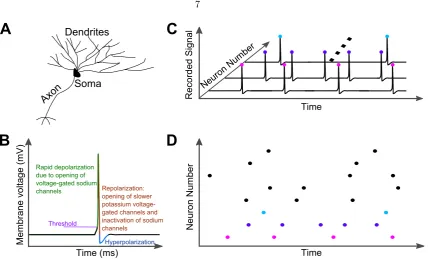
The nervous system of animals, just as all other systems and organs, is composed of organic biological cells. The most studied cells, neurons, can be described analogously to a com-munication system that has a receiver, processor, and transmitter. Such a description is, of course, a simplification, as neurons show vast diversity with various properties [Ram´on y Cajal, 1888, 1933]. For the introduction herein, however, we will view them in this most basic form (see Figure 1.1A).

(14)

1.1.2 What is an action potential?

Since first being reported [Adrian and Zotterman, 1926], neuroscientist around the world now record action potentials daily. The seminal work of Alan Hodgkin and Andrew Huxley provided a leap in our knowledge of action potentials [Hodgkin and Huxley, 1952]. To understand these electrical impulses of communication, one must know that neurons at rest have a net negative charge relative to the external milieu to result in a membrane voltage of approximately -65mV [Bertil, 2001; Johnston and Wu, 1995; Kandel et al., 2013; Koch, 1999]. This potential difference arises due to the relative concentration of ionic species between the inside and outside of cells. Overall, there is a net excess of positively charged sodium ions in the extracellular space that have a net electrochemical concentration gradient driving them inside cells. On the other hand there is a higher concentration of positively charged potassium ions within the cells (relative to the extracelluar space) that have a net electrochemical concentration gradient driving them to leave neurons [Bertil, 2001; Johnston and Wu, 1995; Kandel et al., 2013; Koch, 1999]. This gradient is energetically maintained by ATP-sodium-potassium pumps that line neuronal cell membranes and pump sodium ions out of and potassium ions into cells [Johnston and Wu, 1995; Kandel et al., 2013; Koch, 1999]. As described below, it is the transient passage of sodium and potassium ions through the neuronal membrane that is responsible for the generation of action potentials. Finally, there are also large negatively charged proteins inside and chloride ions outside neurons that contribute to the overall electrochemical gradients and membrane potential though they play less of a role in the rapid dynamics of action potentials [Johnston and Wu, 1995; Koch, 1999].

(15)

TimeA

Neuro

nANumbe

r

C

B

Hyperpolarization

TimeA(ms)A

RapidAdepolarizationA dueAtoAopeningAofA voltage-gatedAsodiumA

channels Repolarization:A

openingAofAslowerA potassiumAvoltage-gatedAchannelsAandA inactivationAofAsodiumA channels

Threshold

A

Axon

Soma Dendrites

D

....

TimeA

Record

edASign

al

Neuro nANumbe

r

Memb

raneAvol

tageA(mV

[image:15.595.108.537.55.314.2]

)AA

Figure 1.1: Neurons, action potentials, and raster plots. (a)Schematic of a neuron showing the dendrites, soma, and axon. The reader should be aware that this is just a stereotypical neuron diagram and that neurons are actually found in a variety of sizes and morphologies [Ram´on y Cajal, 1888, 1933]. (b)Schematic of an action potential describing the different phases. Action potentials in vivo are in the order of 1ms in duration. (c) Illustration of many neurons recorded simultaneously and how action potentials can be identified for each neuron and recorded (colored dots). (d) Example raster plot which is a compression of the information in(c) by only representing the neurons and the time of action potentials. Note the y-axis can also be trial number if, for instance, a single neuron was recorded from multiple times in response to an identical stimulus.

(16)

1.1.3 What are synapses?

The variation in the number of neurons between animal species is vast, from the hundreds to the billions. The round worm Caenorhabditis elegans, a popular organism for neurosci-entific study, has 302 neurons [White et al., 1986], the fruit fly, Drosophila melanogaster, has approximately 135,000 [Alivisatos et al., 2012], while mice and humans brains have 71 million [Herculano-Houzel et al., 2006] and 86 billion [Azevedo et al., 2009] neurons, respectively. To understand the mechanisms underpinning behavior and higher cognitive abilities that arise from these neurons, scientists also need to understand how these neurons are connected. The connection junction between two neurons is called a synapse.

It is critical to note that connectivity is not the last step in explaining the complexity of the brain. For instance, synapses can be of different types, the main division being electrical and chemical synapses [Kandel et al., 2013]. Electrical synapses refer to physical attachment between two neurons at regions termed gap junctions. These connections have cytoplasmic continuity between both cells. As such electrical signals between neurons can cross due to the electrical continuity [Kandel et al., 2013]. Chemical synapses, which are more abundant, have the presynaptic neurons release chemicals called neurotransmitters from synaptic vesicles. These neurotransmitters diffuse across the synaptic cleft, tiny space between the pre and postsynaptic neurons, and bind to postsynaptic neuron channels causing them to open and either hyperpolarize or depolarize the postsynaptic compartment via the passage of ionic species [Kandel et al., 2013]. Contrary to electrical synapses, chemical synapses are unidirectional. Frequently, neurons are categorized based on their synaptic properties [Harris and Shepherd, 2015]. One basic categorization of neurons is grouping them into excitatory and inhibitory neurons. Excitatory neurons release neurotransmitters that will depolarize neurons promoting the initiation of action potentials. Antagonistically, inhibitory neurons release neurotransmitters that hyperpolarize postsynaptic compartments and inhibit the ability of the post-synaptic neuron to send an action potential [Harris and Shepherd, 2015; Kandel et al., 2013; Roux and Buzsaki, 2015].

Given the diversity and intricateness of brains, it is not surprising that a whole field in neuroscience exists to try and uncover the complete neuronal connectivity of animals called connectomics [Behrens and Sporns, 2012]. The term connectome, in parallel to genome, refers to the complete neuronal connectivity map of organisms [Sporns et al., 2005]. As of today, the only species to have its connectome fully determined is that of the roundwormC. elegans [Seung, 2012; Varshney et al., 2011; White et al., 1986]. As will be discussed below, diverse technologies allow the connectome to be approximated at a spectrum of scales and this thesis focuses at three different levels.

(17)

consequences on information transmission and integration for an animal [Seung, 2012]. For instance, the retina connects and transmits information to higher visual brain structures via a bundle of neuronal fibers called the optic nerve [Selhorst and Chen, 2009]. If an optic nerve is damaged and no longer able to transmit information, then an animal will be blind in that eye. Other examples are Parkinson’s disease which is caused by death of dopaminergic (dopamine producing) neurons in a brain structure called the substantia nigra [Davie, 2008] and Alzheimer’s disease characterized by a reduction in the amount of long-range neuronal connections and overall neuronal death [Yao et al., 2010]. Other neurological conditions such as obsessive compulsive disorder and schizophrenia are also thought to be a result of abnormal wiring of the brain [Bullmore and Sporns, 2012].

At this point, I hope the reader has developed an appreciation to the complexity of neuronal networks. The connectivity is vital in determining the emergent properties of the network as discussed below.

1.1.4 What are raster plots?

There are numerous ways to collect neuronal data. Often, neuroscientist are only interested when neurons fire action potentials and this data can be represented in a raster plot as illustrated in Figures 1.1C and 1.1D. Raster plots can be thought of as compressing the data by removing the membrane voltage axis as researchers may not be interested in the waveform of spikes (identical and hence lack information) or subthreshold dynamics of neurons. Thus, time is on the x-axis, whereas the y-axis is discretized and commonly represented as neuron number (Figure 1.1D). Every neuron would be assigned a number and each time a neuron spikes, a dot (or vertical line) is used to represent that spike at a given time. The y-axis can also be trail number if the data was collected from a single neuron while a stimulus was repeated many times. Raster plots are introduced here as they are seen in more than half of the figures in this thesis.

1.2 Brain Networks

(18)

1.2.1 Subcellular networks

The discoveries made about the inner workings of neurons are simply remarkable. The complexity is appreciated by looking at the genetic expression patterns of neurons and how different genes interact (via protein production) and influence one another [Cooper-Knock et al., 2012; Tasic et al., 2016]. The genetic expression patterns govern the cell development processes in addition to a cell’s overall properties and hence cell-type [Ronan et al., 2013]. Recent work has shown that the genetic level is not the only one of interest and that transcript and protein network expressions are vital [Tasic et al., 2016], the focus of the fields of trancriptomics [Cooper-Knock et al., 2012] and proteomics [Prescott et al., 2014]. There are also remarkable intricacies seen at postsynaptic membranes termed postsynaptic densities [Kennedy, 2000]. Here, the mechanisms and interactions of proteins within the cell and on the cell membrane are vast and dynamically changing at all times in response to internal and external stimuli.

Although this scale is not considered in this thesis, it is a field of neuroscience that garners a lot of attention and research. In analogy to airports, which will be done throughout this section, these networks can be thought as the internal operations of every airport individually such as the handling of luggage, gate assignment, terminal transfers, and other processes that keep the complex airport itself functional.

1.2.2 Microscopic networks

On neuronal scales, there is much interest in knowing the full connectivity at a synaptic level between all neurons as done forC. elegans [Seung, 2012; Varshney et al., 2011; White et al., 1986]. Current technologies are able to attain such information very slowly where animal brains can be sectioned into very thin slices (∼25nm thick) and then imaged using electron microscopy [Briggman et al., 2011]. Once this is done for consecutive of slices, neurons are identified using semi-automated methods to trace the shape of every neuron in every slice, determine where they end and connect to other neurons to identify synapses [Denk et al., 2012]. This not only gives the full connectivity (microscopic network) but also the morphology of all cells.

(19)

assemblies in networks, i.e., groups of neurons that show long-lived, coherent co-activity. Specifically, the chapter characterize the appearance of slow-switching assemblies (SSA) in leaky-integrate-and-fire (LIF) neuronal networks, i.e., a coherent increased firing in sub-groups of neurons, sustained over long times and switching from group to group across the network.

Chapter 3 further shows that the ability of clustered LIF networks to support SSA activity can be determined by evaluating spectral properties of the connectivity matrix. I illustrate that the strength of SSA activity can be linked to the existence of a gap separating the leading eigenvalues, together with a block-localization of the associated Schur vectors of this matrix on the neuron groups acting coherently.

To understand the relevance of the connectivity eigen-gap, I consider stylized firing rate models and use the analytical insights they provide to develop LIF networks based on com-pletely different topological and functional connectivity paradigms, which are nonetheless able to display SSA activity (e.g., SSA dynamics involving excitatory and inhibitory neurons, or SSA activity with a hierarchy of timescales).

The findings can be used to indicate if a network can support SSA activity based on spectral analysis which is relevant, for example, in the emergence of oscillations so crucial for information processing in the brain [Buzsaki and Moser, 2013]. Furthermore, this knowl-edge can be used to propose distinct types of topologies of relevance in neuroscience, which can display SSA dynamics. The Chapter illustrates that advancements in neuronal moni-toring and connectomics go hand-in-hand to facilitate our understanding of the relationship between structure, dynamics, and function.

1.2.3 Mesoscale networks

(20)

et al., 2015; Oh et al., 2014]. Using the airport analogy, this is equivalent to identifying how certain overall regions with some airports are connected to other regions without knowing which airports in particular. For instance, one may know there are flights between Southern California and the New York city area, without knowing any specific flights or which of the airports are actually connected. The strength of these connections can still be estimated as they will be proportional to the number of flights between the two regions. Similarly in mesoscale networks, the strength of connections can be estimated by the fluorescent signals at target areas [Kuan et al., 2015; Oh et al., 2014].

In Chapter 5, the effect of chronic sleep deprivation during adolescence on brain mesoscale connectivity is investigated. In this study, a control group and a sleep deprived group (dur-ing adolescence) of mice are compared. After normaliz(dur-ing for inherent experimental and biological noise, I observe that sleep restriction did not alter the mesoscale connectivity be-tween secondary motor cortex (site of injection in this data set) and the rest of the brain in a unitary manner. Using a novel classification algorithm allowed the identification of the two groups significantly above chance level indicating long lasting global changes in the brain do occur due to chronic sleep deprivation in adolescence. The changes are intricate and not a simple overall effect. To further unravel the differences between both groups it may be necessary for future work to develop new analysis techniques, more sensitive recording methodologies and injection techniques, or inject in multiple brain locations. In brief, the age-old advice of not sacrificing sleep was further verified and a step was taken towards understanding how sleep deprivation affects brain connectivity.

1.2.4 Macroscopic networks

(21)

2007; Bassett et al., 2011].

In the aeronautical analogy, this is an even coarser resolution than the above mesoscale connectome where for instance flight connectivity might be identified on a country/continent scale. For instance, are there direct flight connections from Europe to Australia? The work presented herein does not include modeling or analysis of macroscopic networks although this is a vibrant field of neuroscience that is essential in expanding our understanding of the brain.

1.2.5 Functional networks

Networks can also be considered on more abstract levels beyond physical connectivity. Al-though topology constrains the activity a network can exhibit, it is nonetheless the activity of the network that allows for our sensory and cognitive abilities. From one viewpoint, neu-rons may or may not be connected, but their activity can be correlated such that they appear to perform related functions. As such, based on the similarity of neuronal activity, metrics (statistical associations) can be defined between neuron pairs that identify how functionally connected they are [Bullmore and Sporns, 2009]. When this is done for all neurons, a func-tional network is said to be determined. Of course this is less absolute compared to actual physical connectivity as the actual metric used will alter the estimated functional network. Nonetheless, the notion is very useful and is also implemented at larger scales using tech-nology such as functional magnetic resonance imaging (fMRI) or electroencephalography (EEG) [Betzel et al., 2012; Bullmore and Sporns, 2009; Chu et al., 2012].

Continuing with the airport analogy, functional networks are equivalent to finding air-ports with similar activity but are not necessarily connected to each other. This may be of interest to certain researchers as these airports may provide similar overall roles for the network at large and as such want to be identified together. An example is small airports that train pilots in addition to being strategically located for emergency landings. Other examples such as large airports might also form a group and may in fact be connected by direct flights, though in this analysis they are grouped due to similar behavior and not physical connectivity.

(22)

in order to gain insight into the way neural processing and computations are performed at the population level [Buzsaki, 2010; Hebb, 1949]. The technique works on neuronal spiking data applicable across a spectrum of relevant scales that are gathered from modern systems neuroscience experiments. Initially, a novelbiophysically inspired measure is used to extract directed functional relations betweenboth excitatory and inhibitory neurons based on their spiking time history. Second, the resulting induced network representation is then analyzed using a graph-theoretic community detection method to reveal groups of related neurons (cell assemblies) in the recorded time series atall levels of granularity, without prior knowl-edge of their relations or expected size. The methodology is extensively assessed through synthetic, simulated, and experimental spike-train data and highlights the advantage of the functional network perspective in finding neuronal communities based on associated activities.

1.2.6 Feedforward networks

A commonly studied architecture that can also be observed at multiple scales is feedforward networks. The topology of such networks is designed such that information is transmit-ted consecutively along groups (layers) [Kumar et al., 2010; Vogels et al., 2005]. Examples are seen in visual processing where one path of information propagation traverses from the retina to the dorsal lateral geniculate nucleus to the visual cortex [Grubb et al., 2003; Hendry and Reid, 2000]. Another common example is the hippocampus that receives input from the entorhinal cortex that is connected dentate gyrus to the CA3 region to the CA1 re-gion [Llorens-Martin et al., 2014; Olsen et al., 2012]. In the airport analogy, the information can be considered as individual travels. People who are traveling around the world might be restricted from their travel agent to only go in one direction around the planet. As such, the travelers (information) have restricted paths and can only move from one region to the next in a parallel manner to feedforward networks. Scientists have investigated these networks for decades as prototypical examples of how information could be propagated within an organism. Numerous computations and theories have been developed and studied, making this a very advanced and elegant field of research [Kumar et al., 2010; Vogels et al., 2005].

(23)

transmis-sion whose activity centrally involves inhibitory neurons and their connectivity structure, while excitatory neurons remain randomly connected between each other. Specifically, the findings point to the fact that feedforward activity observed in the brain might be caused by a much broader architectural basis than has been considered.

1.3 Recapitulation

(24)

Chapter 2 Revealing cell assemblies at

multiple levels of granularity

Some or all of the work presented in this chapter has been published [Billeh et al., 2014]. This publication is an open access article distributed under the terms of the Creative Commons Attribution License, which permits unrestricted use, distribution, and reproduction in any medium, provided the original author and source are credited.

2.1 Abstract

Identifying cell assemblies, or groups of neurons that cooperate within large neural popula-tions, is of primary importance for systems neuroscience. We introduce a simple biophys-ically inspired measure to extract a directed functional connectivity matrix between both excitatory and inhibitory neurons based on their spiking history. The resulting network representation is analyzed using a graph-theoretical method for community detection to reveal groups of related neurons in the recorded time-series at different levels of granular-ity, without a priori assumptions about the groups present. We assess our method using synthetic spike-trains and simulated data from leaky-integrate-and-fire networks, and exem-plify its use in experimental data through the analysis of retinal ganglion cells of mouse and salamander, in which we identify groups of known functional cell types, and hippocampal recordings from rats exploring a linear track, where we detect place cells with high fidelity.

2.2 Introduction

(25)

links between topology and dynamics of neural interactions, which underpin the functional relationships within neural populations. One such example is the activity of cell assemblies. The problem is to identify groups of neurons (termed cell assemblies) within a large number of simultaneously recorded neurons where, due to functional cooperativity, each cell in an assembly is more similar in its temporal firing behavior to members of its own group than to members of other groups. Such strongly intertwined activity patterns are believed to underpin a wide range of cognitive functions [Buzsaki, 2010; Harris, 2005; Hebb, 1949]. However, the reliable identification of cell assemblies remains challenging.

Here we introduce a technique to identify such neuron assemblies directly from multi-variate spiking data, based on two steps: the definition of a simple biophysically-inspired similarity measure obtained from the observed spiking dynamics, followed by its analysis using a recent framework for multiscale community detection in weighted, directed graphs. A variety of techniques have been proposed to cluster spike-train groups to date, and have shown promising results in particular settings [Abeles and Gat, 2001; Feldt et al., 2009; Fellous et al., 2004; Gansel and Singer, 2012; Humphries, 2011; Laubach et al., 1999; Lopes-Dos-Santos et al., 2011, 2013; Peyrache et al., 2010; Quiroga and Panzeri, 2009]. In contrast to these techniques, our methodology provides a dynamics-based framework, in which both the similarity measure and the community detection method are geared towards incorpo-rating key features of neural network dynamics. The framework is purposely designed to be simple, yet capturing a breadth of features not present concurrently in other methods.

Our similarity measure evaluates the association between neuron pairs based on their spiking history and integrates three features that are key for a network-based analysis of neuro-physiological data: (i) an intuitive biophysical picture, allowing a simple interpreta-tion of the computed associainterpreta-tions; (ii) a measure that is directed in time, hence asymmetric in the sense that spike-time dependent information is retained (e.g., spiking of neuron A precedes that of neuron B); (iii) excitatory and inhibitory interactions are both included yet treated differently, inspired by their distinct effects on post-synaptic cells.

(26)

hippocampal pyramidal neurons.

2.3 Materials and Methods

Most existing methods to detect groups in spike-train neuronal population data are based on the following generic paradigm [Feldt et al., 2009; Fellous et al., 2004; Humphries, 2011; Lopes-Dos-Santos et al., 2011]. First, a metric is defined to quantify the relationship between all neuron pairs leading to aN×N association matrix, whereN is the number of observed neurons. We call this the functional connectivity matrix (FCM) hereafter. Every (i, j) entry in this matrix is a non-negative number that indicates how similar the spike trains of neuronsiandj are over the observed time. Second, the FCM is clustered,i.e., partitioned into different groups [Aggarwal and Reddy, 2014; Fortunato, 2010; Newman, 2004].

Here we introduce a simple framework that addresses both of these steps in a consistent and integrated manner, focusing on the dynamical relations between neurons: a new directed (‘causal’) biophysically-inspired measure is introduced to calculate the FCM, which is then analyzed using the recently introduced dynamics-based technique of Markov Stability for community detection [Delvenne et al., 2013, 2010; Lambiotte et al., 2009; Schaub et al., 2012] to identify cell assemblies at multiple scales in the neuronal population.

The numerics are performed in MATLAB (2011b or later versions). Code implementing the algorithm for spike-train analysis is available upon request and can be found at:

github.com/CellAssembly/Detection.

2.3.1 Biophysically-inspired causal measure of spike-train

similar-ity

(27)

Excitatory Coupling

("EPSP")

Inhibitory Coupling

("inverted EPSP")

a

b

Figure 2.1: Biophysically-inspired measure of spike-train similarity leading to functional coupling between neurons. Quantification of the coupling induced by: (a)excitatory neuron

A on neuronB and(b) inhibitory neuronA on neuronB. Note that both profiles shown are normalized so that the signal has zero mean (see text).

While an even finer characterization of neuronal subtypes could be of further interest, the distinction between excitatory and inhibitory neurons underpins fundamental balances in neuronal network dynamics and should be reflected in the analysis of data. Here, we propose a similarity measure that incorporates these three ingredients in a simple, intuitive form (see Figure 2.1).

Consider first an excitatory neuron A connected to neuron B. The action potentials of A induce excitatory postsynaptic potentials (EPSPs) in neuron B, increasing the likelihood of neuron B firing. These EPSPs can be, to a first approximation, modeled by an exponentially decaying time profile

ξexc(t) =e−t/τ

with synaptic time constant τ. Since detailed information about synaptic weights and membrane potentials is unavailable in neuronal population experiments, we adopt a simple strategy to compute the coupling strengthSABfrom the observed spiking data. The general idea is that for each spiking event of neuron B (at timetB_i ), we propagate a ‘virtual’ EPSP from the immediately preceding spike of neuron A (at timetA_i). We then compute all such contributions that neuron A would have made to the membrane potential of neuron B at each of its spikes, and sum them appropriately, discounting spurious effects.

More precisely, we obtain the functional connectivity from neuron A to neuron B as follows:

(28)

firing event at any other neuron taking place at timet:

fA(t) =ξexc(t−tAlast) =e− (t−tA

last)/τ_, _(2.1)

where tA

last= maxi(tAi |tAi ≤t), i= 1, . . . , NA, is the time of the last preceding spike of

neuron A (if there is no such spike we settA_last=−∞).

(ii) It then follows that all contributions from neuron A to B can be written as the sum

PNB

i=1fA(t B

i ). To gain some intuition, note that every time B fires a spike, the potential

contribution to this spike by neuron A is computed by summing the values that fA(t)

takes at the times of B firing, tB

i . If neuron B always fires shortly after A spikes, the sum

PNB

i fA(tBi ) will be large. If neuron B fires after A but with some delay (e.g., because an

integration with other neurons is required), this sum will be smaller. If neuron B never fires shortly after A, this sum will be zero.

To discount spurious correlation effects, we center and normalize the signal fA(t) first to obtain the new signal ˜fA(t), which has zero mean and peak amplitude one (Figure 2.1a)

˜

fA(t) =

fA(t)− hfAi

1− hfAi

, (2.2)

wherehfAi= _T1 R₀TfA(t)dt≤1 is the mean over the recorded time. We then compute the effective coupling:

FAB =

1

NAB NB

X

i=1

˜

fA(tBi ), (2.3)

and we have additionally divided by NAB = max(NA, NB) to guarantee that the maximal coupling FAB (between two identically firing neurons) is normalized to 1. The coupling between neuron A and B is then defined as the thresholded value:

SAB= max(FAB,0). (2.4)

From this definition, it follows that if an action potential from neuron A is always closely followed by a spike from neuron B, this will correspond to a strong coupling SAB

between these neurons. Note that, in addition to being biophysically inspired, the defined measure (2.4) is non-symmetric (SAB6=SBA).

(29)

this influence, we adopt an ‘inverted’ exponential profile

ξinh(t) = 1−e−t/τ,

truncated when it reaches 99% of its steady state value. Hence, if neuron B always fires shortly after the firing of the inhibitory neuron A, it will accumulate a negative dependence from which we deduce that there is no significant inhibitory functional relation between these neurons.

The time scale τ is a parameter inspired by synaptic time constants, and can thus be adapted to reflect prior information about the recorded neurons. Although more sophisti-cated schemes to estimate or tune this parameter are certainly possible (e.g., choosing a different τexc for excitatory and τinh for inhibitory neurons), here we follow the simplest

choice τexc=τinh=τ throughout. The method is robust to the choice ofτ: we have used τ = 5 ms for the experimental data and τ = 3 ms for the leaky-integrate-and-fire (LIF) simulation data, and have checked that the results remain broadly unaltered for values ofτ

in this range.

The main aim of our measure is simplicity, flexibility and generality, while retaining the key biophysical features outlined above. Because of its generality, highly specialized measures of spike-train associations could be tuned to outperform our simple measure for particular examples. However, it is often unknown beforehand what features of the data are of importance for the analysis and hence having such a flexible measure allows for a broad search for structure in recorded data. Once a hypothesis is formed, or particular aspects need to be investigated in more detail, more specialized association metrics could be used in conjunction with the community detection algorithm presented below. In the absence of knowledge about the specific cell types of experimentally recorded neurons we obtain the FCM using the excitatory metric. Already today, however, there are means to separate cell types (e.g. fast spiking interneurons) based on their electrophysiological signature [Barth´o et al., 2004] and with the advancement of optical physiology and genetic tools, additional information about the cell types of the recorded cells is becoming more routine. Hence it will be possible in the future to use specialized coupling functions (instead of exponential) depending on the neuronal sub-type recorded.

2.3.2 Markov Stability for community detection at all scales

(30)

we extend the use of Markov Stability to directed networks to find coherent groupings of neurons in the FCM created from the observed spiking data. Under our framework, we interpret the FCM as a directed network, and the graph communities revealed by our anal-ysis correspond to groups of neurons with strong excitatory and/or inhibitory couplings extracted from the dynamics. Therefore the graph partitioning problem solved using the Markov Stability method is linked to the detection of putative cell assemblies,i.e., groups of neurons with a strong dynamical influence on each other.

The main notion underpinning the Markov Stability method is the intimate relationship between structure and dynamics on a graph. A dynamics confined to the topology of a network can uncover structural features of the graph by observing how a dynamical process, such as a simple diffusion, unfolds over time. In particular, if the graph contains well defined substructures, such subgraphs will trap the diffusion flow over a significantly longer time than expected if it were to happen on an unstructured graph. This idea is readily illustrated by the example of ink diffusing in a container filled with water. If the container has no structure, the ink diffuses isotropically. If the container is compartmentalized, the ink would get transiently trapped in certain regions for longer times until it eventually becomes evenly distributed throughout. In a similar manner, by observing the dynamics of a diffusion process we can gain valuable information about the structural organization of the graph (Figure 2.2). We use this concept to define a cost function to detect significant partitions in the graph, as follows.

To make these notions precise, consider a network with a Laplacian matrix L=D−A, whereAis the weighted adjacency matrix (Aij is the weight of thedirected link from node

ito nodej) andD = diag(A1) is the diagonal out-degree matrix (1is the vector of ones). For ease of explanation, consider first a strongly connected graph,i.e., we can traverse the graph along its directed edges such that every node can be reached from any other node. On such a network, let us define a continuous diffusion process:

˙

p=−pD−1L, (2.5)

wherepis the 1×Nprobability vector describing the probability of a random walker to visit different nodes over time. Note that the probability vector remains properly normalized:

1Tp = 1 at all times. For an undirected connected graph, this dynamics converges to a unique stationary distributionπ=d/(dT1). Fordirected graphs the stationary distribution has to be computed by solvingp˙ = 0,i.e., it corresponds to the dominant left eigenvector of D−1_L_{. If the graph is not strongly connected (e.g., if it contains a sink), the diffusion}

(31)

Dynamics evolving with increasing Markov time Analyzed Graph

10−2 10−1 100 101 102

100 101 102

Markov time

No

. of com

m

un

itie

s

18

6

2

a

b

VI

0.1

[image:31.595.185.430.57.278.2]

..

Figure 2.2: Schematic of Markov Stability method used to partition the functional network.

(a) A diffusion process on a network can be used to reveal the structure of a graph. As the diffusion explores larger areas of the network, it enables the Markov Stability method to scan across all scales and reveal relevant partitions at different levels of granularity. (b)

The graph analyzed has a pre-defined multi-scale community structure, given by a hierarchy of triangles. The number of communities found are plotted as a function of the Markov time (see (a)) long plateaus indicate well-defined partitions into 18 nodes (each node on its own), six communities (small triangular structures), and two communities (aggregated, larger triangles). Note that in this example, the variation of information (VI) is zero for all Markov times, indicating that all three partitions are relevant at different levels of resolution. We remark that the sudden steps between plateaus is a result of the specific example chosen. Since many of the weights were chosen to be identical, there is a lot of symmetry in the graph which results in many repeated eigenvalues in the stability matrix. This causes the sharp transition between plateaus during the Louvain optimization step (see text). The addition of a small amount of variation in the weights would result in a smooth transition between plateaus (provided Markov time is sampled finely enough).

by Google’s page-rank algorithm [Brin and Page, 1998; Lambiotte et al., 2009; Lambiotte and Rosvall, 2012]: the random walker is transported from any node to a random node in the graph with a small, uniform probability α (set here to the commonly adopted value

α= 0.15), while in the case of a sink node, it will be teleported with unit probability. This term guarantees that the process is ergodic with a unique stationary probability distribution. Consider a partition of this network encoded in aN×cindicator matrixH, withHij = 1 if node i belongs to community j. We then define the Markov Stability of the partition

r(tM, H), as the probability that a random walker at stationarity starts in community i

and ends up in the same community after time tM minus the probability of such an event

happening by chance, summed over all communities and nodes. In matrix terms, this may be expressed as:

(32)

r(tM, H) = traceHTS(tM)H,

where Π = diag(π) andtM denotes the Markov time describing the evolution of the diffusion process. Finding a good partition (or clustering) requires the maximization of the Markov Stability in the space of possible graph partitions for a given tM, an optimization that can be carried out with a variety of optimization heuristics. Here we use a locally greedy optimization, the so-called Louvain algorithm, which is highly efficient [Blondel et al., 2008]. In order to deal with the fact thatS(tM) is in general asymmetric due to the directed nature of the graph, we use the directed notion of Markov Stability and use the Louvain algorithm to optimizeHT1

2(S+S

T₎_H_{, which is mathematically identical to optimizing}_r₍_t

M, H), i.e.,

we still consider thedirected network.

Our algorithm then scans across all Markov times to find the set of relevant partitions at different Markov times. With increasing Markov time, the diffusion explores larger regions of the network, resulting in a sequence of increasingly coarser partitions, each existing over a particular Markov time scale. The Markov time may thus be interpreted as a resolution (or granularity) parameter, and, as we sweep across resolutions, we detect communities at different levels of granularity without imposing a particular resolution a priori. This dynamic sweeping [Schaub et al., 2012] allows us to detect assemblies of different sizes and even hierarchical structures that would potentially go undetected if we were to use a method with a fixed intrinsic scale [Feldt et al., 2009; Fellous et al., 2004; Fortunato and Barth´elemy, 2007; Humphries, 2011; Lopes-Dos-Santos et al., 2011; Newman and Girvan, 2004]. It is important to remark that the Markov timetM used for the diffusive exploration of the network is not to be confused with the physical time of the spike-train dynamics. We remark that the time constantτ of our similarity measure is not related to the Markov time in general. The Markov time is used here as a tool to uncover the different scales in the data and should thus be seen as distinct from the biophysical (real) time.

(33)

a standard tool to compare partitions in the context of community detection [Fortunato, 2010]. The normalized VI between two partitionsPα _and_Pβ _{is defined as [Meila, 2007]:}

VI(Pα_,_Pβ_{) =} 2H(P

α_,_Pβ₎₋_H₍_Pα₎₋_H₍_Pβ₎

logN , (2.6)

where H(P) =−P

Cp(C) logp(C) is the Shannon entropy of the relative frequencyp(C) = nC/N of a node belonging to communityC in a partitionP andH(Pα,Pβ) is the Shannon

entropy of the corresponding joint probability. We then calculate the average variation of information (V I) over all pairs in the ensemble of solutions from the optimization. When

V I≈0, the solutions obtained by the different optimizations are very similar to each other indicating a robust partitioning. When V I ≈ 1 each run of the optimization obtains a different partition, indicating a non-robust clustering. Such clear-cut communities are not always found. However, we have shown [Delmotte et al., 2011; Schaub et al., 2012] that sudden drops and dips in theV I are indicative of a clustering becoming more robust than expected for its average community size. In realistic datasets, we thus search for partitions with a long Markov time plateau and a low value (or a pronounced dip) of V I as the criterion to find meaningful partitions. An illustration of the Markov Stability framework is displayed in Figure 2.2b, where we exemplify how the graph community structure can be detected at different scales withouta priori assumptions about the number of communities. Furthermore, our scanning across all Markov times allows for the detection of the appropriate scale for community detection, without imposinga priori a particular scale that might not be relevant to the analyzed data, as is implicitly done in other methods [Schaub et al., 2012].

2.3.3 Synthetic spiking data

To assess the capabilities of the framework, we generated synthetic spiking datasets with realistic statistical properties resembling those observed in experiments, yet with added temporal structure.

2.3.3.1 Synthetic data with embedded and hierarchical cell assemblies

Surrogate spike-train data were created from groups of units with variable sizes. Each group

Giwas assigned a firing rate (fi) and a level of jitter (Ji). The firing times of eachgroupwere drawn from a uniform distribution according to the specified firing frequency fi, and the

firing times for eachunit were chosen from a uniform distribution with a range±Jiaround

(34)

into two subgroups: units within each subgroup always fire together, whereas between two subgroups the firing window was aligned only every second time. As before, the firing times of the individual groups were chosen randomly from a uniform distribution and were not correlated in time. This firing pattern establishes a two-level hierarchical relation between the individual units.

2.3.3.2 Synthetic data with feedforward-like firing patterns

Synthetic spiking patterns that emulate the activity of feedforward networks were created from groups that are made to spike together within a jitter window of±1 ms. The groups are set to spike sequentially with a delay ofδ = 5 ms and a repetition period of ∆ = 20.5 ms.

2.3.4 Simulated data from Leaky-Integrate-and-Fire Networks

We applied our algorithm to more realistic spiking computational datasets obtained by simulating neuronal networks of excitatory and inhibitory Leaky-Integrate-and-Fire (LIF) neurons [Koch, 1999].

2.3.4.1 The excitatory and inhibitory LIF units

The non-dimensionalized membrane potentialVi(t) for neuronievolved according to: dVi(t)

dt =

µi−Vi(t)

τm +IS, (2.7)

where the constant input term µi was chosen uniformly in the interval [1.1,1.2] for exci-tatory neurons and in the interval [1,1.05] for inhibitory neurons. Both excitatory and inhibitory neurons had the same firing threshold of 1 and reset potential of 0. Note that although the input term is supra-threshold, balanced inputs guaranteed that the average membrane potential remained sub-threshold [Litwin-Kumar and Doiron, 2012; van Vreeswijk and Sompolinsky, 1998]. Membrane time constants for excitatory and inhibitory neurons wereτm= 15 ms andτm= 10 ms, respectively, and the refractory period was 5 ms for both

excitatory and inhibitory neurons. The synaptic input from the network was given as:

IS= X

i←j

wi←jgjE/I(t), (2.8)

where thei←jdenotes that there is connection from neuronjto neuroni, andwi←jdenotes

the weight of this connection (see next section for the weight settings). The synaptic inputs

(35)

a

b

c

Inhibitory Excitatory

…

… …

…

Inhibitory Excitatory

E-E Clustered LIF E-E Hierarchical LIF E-I Clustered LIF

…

Excitatory

Inhibitory

Figure 2.3: Schematic wiring diagrams of the three LIF networks used in this work: (a)an E-E clustered LIF network; (b) an E-E hierarchical LIF network; (c) an E-I clustered LIF network. Arrow thickness is proportional to the strength of the connection. For the parameters used in our simulations, see Table 2.1.

and then decayed exponentially according to:

τE/I dgE/I

dt =−g

E/I₍_t₎_, _(2.9)

with time constantsτE= 3 ms for an excitatory interaction, andτI = 2 ms if the presynaptic unit was inhibitory.

2.3.4.2 Network Topologies and Weight Matrices

LIF excitatory and inhibitory units in a proportion of 4 : 1 were interconnected with three different network topologies. The resulting networks were simulated with a 0.1 ms time step. The connection probabilities and weights between the different types of neurons for these three LIF networks are shown in Table 2.1 and the schematic of the different wiring diagrams is shown in Fig. 2.3.

Network with clustered excitatory connections (E-E clustered) We first con-structed a LIF network with clustered excitatory units: each excitatory neuron belongs to a group of units more strongly connected to each other than to units outside the group (Figure 2.3a). The network also included unclustered inhibitory units, which ensured that the network was balanced. These networks display temporally-structured spike-train ac-tivity [Litwin-Kumar and Doiron, 2012], and are used here as a test-bed for cell-assembly detection from spiking dynamics.

(36)

Probabilities

pII _pIE _pEI _pEE _pEE

sub pEEsub,sub pEIsub pIEsub

E-E Clustered 0.5 0.5 0.5 0.167 0.5 — — —

E-E Hierarchical 0.5 0.5 0.5 0.15 0.3 0.99 — —

E-I Clustered 0.5 0.454 0.526 0.2 — — 0.263 0.90

Weights

wII _wIE _wEI _wEE _wEE

sub wEEsub,sub wEIsub wIEsub

E-E Clustered −0.04 0.01 −0.025 0.012 0.0144 — — —

E-E Hierarchical −0.04 0.01 −0.03 0.012 0.012 0.014 — —

[image:36.595.126.485.77.190.2]

E-I Clustered −0.04 0.0086 −0.032 0.0155 — — −0.0123 0.0224

Table 2.1: Parameters for the simulated LIF networks. Connection probabilities (pXY) and weights (wXY_{) between different unit types: excitatory (E) and inhibitory (I),} _e.g., pEI _{is the connection probability from inhibitory to excitatory units. For the clustered}

networks, the average E-E connection probability was kept constant at 0.2. For a schematic representation of the wiring diagrams, see Fig. 2.3.

(Figure 2.3b). For this, we split the population of excitatory units into nested clusters, such that each group was sub-divided into smaller groups with increasing internal connectivity. The inhibitory neurons remained unclustered.

Network with excitation to inhibitory clustered feedback loops (E-I clustered)

Finally, we have developed a LIF network to study the dynamical spiking patterns origi-nated by networks in which excitatory and inhibitory neurons are co-clustered, as shown in Figure 2.3c. In this case, whereas the excitatory-to-excitatory and inhibitory-to-inhibitory couplings were kept uniform, we introduced structural features in the connections between distinct neuron types. In particular, each subset of excitatory units was more strongly con-nected to a subset of inhibitory units. This group of inhibitory units, in turn, had a weaker feedback to its associated excitatory neuron group, as compared to the rest of the graph. Every unit was part of one such functional group comprising both excitatory and inhibitory units.

2.3.5 Experimental data

2.3.5.1 Retinal Ganglion Cell recordings from mouse and salamander

(37)

KCl, 2.5; MgCl2, 1.6; CaCl2, 1; and D-glucose, 10; equilibrated with 95% O2and 5% CO2

gas) at room temperature. The mouse retina was perfused with oxygenated Ame’s medium (Sigma-Aldrich; A1420) at 37◦C.

Recordings were made with a custom-made amplifier and sampled at 10 kHz. Spike sorting was performed offline by analyzing the shape of action potentials on different elec-trodes [Gollisch and Meister, 2008; Pouzat et al., 2002]. The spike-triggered averages (STAs) and receptive fields of the salamander retinal ganglion cells (RGCs) were determined by re-verse correlation to a checkerboard stimulus flickering with intensities drawn from a normal distribution. Singular-value decomposition of the spatio-temporal receptive field allowed the extraction of the temporal filter of every RGC receptive field [Gollisch and Meister, 2008].

2.3.5.2 Hippocampal CA1 and CA3 recordings from rats under a

spatiotem-poral task

We analyzed spike trains obtained by Diba and Buzsaki [2007] from hippocampal neurons of rats moving along a linear track implanted with silicon probe electrodes along CA1 and CA3 pyramidal cell layers in left dorsal hippocampus.

2.3.6 Performance of the method and comparisons to other

tech-niques

In those examples where the results could be compared against a ground truth, the perfor-mance of the method was determined by the percentage of correctly classified neurons (hit rate) relative to the true membership in the data.

We have compared the performance of our methodology with two other popular commu-nity detection techniques: modularity optimization (two variants) using the code provided and explained in [Humphries, 2011], and standard agglomerative hierarchical clustering us-ing the nearest distance linkage criterion as implemented in MATLAB.

2.4 Results

2.4.1 Assessing the algorithm with synthetic datasets

(38)

a

T ra in ID 200 400 600 800

c

Time (s) Re -or der ed I D 200 400 600 800

0 1 2 3 4

Time (s)

b

Reordered Neuron ID

Re or d er e d Ne ur o n I D Neuron ID Ne ur o n I D 800 200 400 600 400 200 600 800 0 0.05 0.1 0.15 0.2 800 200 400 600 400 200 600 800 0 0.05 0.1 0.15 0.2 7

100 101

100

101

102

103

10−2 10−1 0

0.05 0.1 0.15 Markov time VI No

. of Com

m

u

ni

ties

Unordered FCM

Markov Stability Analysis

[image:38.595.121.493.72.351.2]

Re-ordered FCM

Figure 2.4: Markov Stability analysis of a synthetic data set. (a)Unsorted raster plot of a population of 800 spike-trains obtained from 7 groups of different sizes. Each ‘cell assembly’ fires at different times with varying amounts of jitter. (b) FCM from the unsorted spike train rastergram, followed by the Markov Stability plot and the FCM reordered according to the partition into 7 groups obtained by the algorithm. Note the long plateau (blue shaded) around Markov time tM = 1 with V I = 0, indicating the presence of a robust partition with 7 groups. At later Markov times, the algorithm detects other robust coarser partitions corresponding to aggregates of the seven groups with similar firing patterns. (c)Color-coded raster plot reordered according to the partition obtained in(b).

2.4.1.1 Analysis of synthetic data with embedded cell-assemblies

As a first illustration, Figure 2.4 shows the application of our method to a synthetic spike dataset with inherent group structure (see Materials and Methods). A population of 800 units was divided into 7 differently sized groups comprising 75 to 200 units. The average spiking frequency for all groups was 12 Hz with±20 ms jitter around the uniformly chosen firing times within the total length of 4 s.

(39)

a

300 Neurons 500 Neurons 800 Neurons

Number of Groups

30 40 50 60 70 80 90 100

0 5 10 15 20 25

% C or rect C la ssifie d

d

b

c

Frequency (Hz)

% C or rect C la ssifie d

100 ₁₀1 ₁₀2

30 40 50 60 70 80 90 100

60 ms Jitter 40 ms Jitter

Time (s)

0 1 2 3 4 5 6 7

30 40 50 60 70 80 90 100

60 ms Jitter 40 ms Jitter

% C or rect C la ssifie d % C or rect C la ssifie d Jitter (ms)

20 40 60 80 100 120

[image:39.595.184.428.57.279.2]

30 40 50 60 70 80 90 100 6 Hz 4 Hz

Figure 2.5: Assessing the performance of the clustering algorithm using synthetic data.

(a) At very low firing frequencies, the classification performance is low due to a small number of spikes per neuron. Performance quickly improves with increasing firing frequency.

(b) The classification performance improves as the duration of the recording increases.

(c) As the jitter increases, the classification performance degrades. (d)The classification performance degrades mildly as the number of groups to be detected increases.

neurons were correctly clustered. Note that the algorithm detects other partitions with relatively long plateaux in Markov time, although their variation of information is non-zero. In particular, a relatively robust partition into three clusters betweentM = 8.21 and

tM = 25.12 is detected corresponding to a coarser grouping of the seven groups embedded in our data.

(40)

a

b

c

0 2 4 6 8 10

Time (s) Ne ur on I D Time (s) Re or der ed Ne ur on I D

Reordered Neuron ID

Re or der ed Ne ur on I D

100 200 300 400 500 50 100 200 300 400 500 0 0.05 0.1 0.15 0.2 0 0.05 0.1 0.15 0.2

100 200 300 400 500 100 200 300 400 500 Ne ur on I D

Neuron ID 10

−1

100 101

100 101 102 103 0 0.02 0.04 0.06 0.08 VI 10 20 No

. of com

m un itie s 100 200 300 400 500 50 Markov time

0 2 4 6 8 10

Re or der ed Ne ur on I D 100 200 300 400 500 50 100 200 300 400 500

[image:40.595.118.496.73.479.2]

0 2 4 6 8 10

Figure 2.6: Detecting hierarchically structured spike train communities in synthetically generated data. Synthetic data of 500 units clustered into 10 groups with 2 subgroups each (20 subgroups in total). (a)Unsorted raster plot of data. (b)Markov Stability analysis of the associated FCM. Clear plateaus indicate the presence of robust partitions into 20 and 10 communities, with classification accuracy of 100% in both cases. (c)Sorted raster plots for the finer (20 groups, top panel) and coarser (10 groups, bottom panel) partitions revealing the hierarchical organization in the data.

(41)

VI

No

. of com

m un itie s 4 Ne ur on I D Neuron ID

50 100 150 200 40 80 120 160 200 0 0.1 0.3 0.5 0.7

c

0 0.1 0.3 0.5 0.7

50 100 150 200 40 80 120 160 200 Reordered ID Re or der ed I D

b

a

Time (s)

0.02 0.04 0.06 0.08 0.1

50 100 150 200 Ne ur on I D Ne ur on I D

0.1 0.2 0.3 0.4

Time

10−1 100 101

1 10 100 0 0.02 0.06 0.1 Markov time Re or der ed I D Time (s)

0.02 0.04 0.06 0.08 0.1

0 40 80 120 160 200 Re or der ed I D

0.1 0.2 0.3 0.4

Time coarse grained

[image:41.595.111.497.75.438.2]

graph

d

Figure 2.7: Analysis of feedforward-like firing patterns. (a) Unsorted raster plot of the synthetic data and zoom-in. (b) Markov Stability analysis of the FCM identifies a robust partition into 4 groups, with 100% classification accuracy. Note that the FCM is asymmetric, thus revealing the directionality of the data. (c)Color-coded raster plot and zoom-in color-coded according to the partition found reveals the feed-forward functional relationship in the data. (d)Coarse-grained representation of the functional connectivity network found from the clustering. For a second example, see supplementary information.

2.4.1.2 Analysis of synthetic hierarchical spiking patterns

(42)

Using the same methodology as above, our analysis reveals two extended plateaus with

V I= 0, for 20 and 10 groups (Figure 2.6b). The sorted raster plots for the 20 and 10 groups, shown in Figures 2.6c, correspond to 100% correct classification. As we will demonstrate below in the context of LIF networks, this consistent multi-scale detection of cell assemblies is a distinct feature of our methodology, which is not present in many other methods which only detect groupings at a particular level of granularity [Fortunato, 2010].

2.4.1.3 Analysis of synthetic feedforward spiking patterns

To highlight the capability of our framework to deal with directed dynamical patterns, we show how feedforward-like functional patterns in the data lead to a pronouncedly asymmet-ric FCM, which can then be analyzed with Markov Stability. Synthetic spiking patterns were generated in which four groups of 50 neurons (with jitter) spiked 20 times, emulating synchronous activity in feedforward networks (see Materials and Methods). As shown in Figure 2.7, our method is able to detect feedforward patterns between cell assemblies: the corresponding Markov Stability plot shows a robust and extended plateau with four com-munities with 100% classification accuracy revealing an effective coarse-grained description of a functional feedforward network.

This is an instance in which the directed nature of our FCM, together with the fact that Markov Stability can detect communities in directed networks, leads to the detection of cell assemblies with directed, causal relationships. Indeed, there are instances of directed functional couplings [Rosvall and Bergstrom, 2008] in which using symmetric measures will lead to different cell assemblies to those obtained if directionality is taken into account. Hence for some networks, directionality is absolutely essential for proper clustering as we consider with a second example.

Figure 2.8a shows the wiring diagram of a network which, if analyzed with a symmetric similarity measure, lead to different cell assemblies that miss the causality/direction of the connections. This network may produce firing patterns as shown in Fig. 2.8b.

There are two possible outcomes when analyzing the raster plot

• When this spike-trains are analyzed using a symmetric measure, leading to a symmetric FCM, we get a partition into two groups: {1,4}and{2,3}, which reflect the strength of the connections but not the causality of the dynamics (see Figure 2.8c).

• When the spike-trains are analyzed using the true, directed FCM, we find the assem-blies based on flow, which illustrates the fact that clearly different clusterings can arise when taking into account directionality (see Figure 2.8d).

(43)

1 2 3 4

a

b

−1 ₁₀ 100 101 102 103

10 0 ₁₀1

0.05 0.1 0.15 −2 100 101 102 103

10 10−1 100 0

0.02 0.04 0.06

c

d

No

. of com

m

un

itie

s

No

. of com

m un itie s VI VI 1 2 3 4 1 2 3 4 Markov time Markov time 2 2 Undirected network analysis

Directed network analysis Functional network

0.1 0.2 0.3

0 50 100 150 ... ... ...

Time / s

Ne

ur

on I

D

40 80 120 160 200 40 80 120 160 200 Neuron ID Ne ur on I D

40 80 120 160 200 40 80 120 160 200 Neuron ID Ne ur on I D 1 2 3 4 1 2 3 4

0.1 0.2 0.3

0 50 100 150 ... ... ...

Time / s

Ne

ur

on I

D

0.1 0.2 0.3

0 50 100 150 ... ... ...

Time / s

Ne

ur

on I

[image:43.595.109.505.62.344.2]

D

Figure 2.8: Comparison of how directionality can affect clustering results. a-bA functional network as depicted in a can be emulated by synthetic data by varying the group firing sequences and delay between individual group firings (b). Ignoring directionality (using the symmetrized FCM) leads to finding assemblies based on the strength between the groups (seec). Taking into account directionality reveals a grouping based on flow (seed).

cases: once we use a symmetric FCM the directions of the links are lost, and thus we can only recover the partition based on strength. Within our framework, the importance of directionality can be tested by including or disregarding directionality in the analysis and comparing the outcomes.

2.4.2 Detecting cell assemblies in simulated networks

Beyond purely synthetic datasets, we now consider three examples of simulated dynamics of LIF networks, which exhibit a range of features of relevance in realistic neural networks. LIF networks provide a simple, controlled testbed to assess our framework on network dynamics broadly used in computational systems neuroscience.

2.4.2.1 Cell assemblies in LIF networks with clustered excitatory connections

Functional, Clustered, Feedforward, and Mesoscale Brain Networks

networks

Yazan N. Billeh

Acknowledgements

Abstract

Published Content and

Contributions

Contents

Chapter 1

Introduction

1.1

Background

1.1.1

What are neurons?

1.1.2

What is an action potential?

C

B

A

D

....

1.1.3

What are synapses?

1.1.4

What are raster plots?

1.2

Brain Networks

1.2.1

Subcellular networks

1.2.2

Microscopic networks

1.2.3

Mesoscale networks

1.2.4

Macroscopic networks

1.2.5

Functional networks

1.2.6

Feedforward networks

1.3

Recapitulation

Chapter 2

Revealing cell assemblies at

multiple levels of granularity

2.1

Abstract

2.2

Introduction

2.3

Materials and Methods

2.3.1

Biophysically-inspired causal measure of spike-train

similar-ity

a

b

2.3.2

Markov Stability for community detection at all scales

a

b

..

..

2.3.3

Synthetic spiking data

2.3.4

Simulated data from Leaky-Integrate-and-Fire Networks

a

b

c

2.3.5

Experimental data

2.3.6

Performance of the method and comparisons to other

tech-niques

2.4

Results

2.4.1

Assessing the algorithm with synthetic datasets

a

c

b