Snowmass benchmark points and three-loop running

arXiv:hep-ph/0408128v1 10 Aug 2004

LTH 628 CERN-PH-TH/2004-153 hep-ph/0408128

Snowmass Benchmark Points and Three-Loop Running

I. Jack, D.R.T. Jones1 and A.F. Kord

Department of Mathematical Sciences, University of Liverpool, Liverpool L69 3BX, U.K.

We present the full three-loop β-functions for the MSSM generalised to include ad-ditional matter multiplets in 5, 10 representations of SU(5). We analyse the effect of three-loop running on the sparticle spectrum for the MSSM Snowmass Benchmark Points. We also consider the effect on these spectra of additional matter multiplets (the semi-perturbative unification scenario).

August 2004

1. Introduction

The LHC will soon resolve the question as to whether low energy supersymmetry is the solution to the hierarchy problem; and if it is, moreover, the LHC and a future e+_e−

linear collider (LC) will lead to very precise measurements of the sparticle spectrum and couplings. The success of gauge unification in the MSSM suggests a Desert, the existence of which would mean that extrapolation of the MSSM couplings and masses to high scales will lead to immediate information about the underlying theory; for example regarding the commonly assumed universality of soft scalar masses, gaugino masses and cubic scalar interactions.

One component of this analysis is the running of masses and couplings between the weak and gauge unification scales, which is governed by the renormalisation group β-functions. In this paper we compare the results for this process using one, two and three-loop β-functions. In each case we generally use the same one-loop corrections for the relationship between running and pole masses for the various particles, with some use of two-loop results such as for the top quark mass. We anticipate that by the time sparticles are discovered complete two-loop threshold corrections will be available; the effect of these we would expect to be of the same order of magnitude as the effect of using the three-loop (as opposed to two-three-loop) β-functions, which, as we shall see, is surprisingly large for squarks.

The plan of this paper is as follows. In section 2 we review the exact results that relate theβ-functions for the soft masses and interactions[1] –[3] to the β-functions of the dimensionless gauge and Yukawa couplings [4]– [6], which we then give through three loops for the MSSM generalised to incorporate n5 andn10 sets of SU5 5(5) and 10(10)

represen-tations respectively. (A motive for grouping additional matter in this way is that complete SU5 representations do not (at one loop) change the prediction of sin2θW (or alternatively

ofg2₃(MZ)) that follows from imposingg1,2,3gauge unification. Also unchanged at one loop

is the gauge unification scale, MX; but at higher loops this scale increases and can

ap-proach the string scale.) We also give a simplified example of a three-loop soft β-function; general results for all the β-functions are available at Ref. [7].

In section 4 we consider the effect of additional matter fields in SU5 representations,

as discussed in Refs. [12], [13] (for earlier work see for example Refs. [14]) and by ourselves in a previous paper [15]. We give some further examples of the effect on the sparticle spectrum of such matter. Finally section 5 contains our conclusions.

2. The Soft Beta functions

For a general N = 1 supersymmetric gauge theory with superpotential

W(φ) = 1₂µij_φ

iφj + 1₆Yijkφiφjφk, (2.1)

the standard soft supersymmetry-breaking scalar terms are as follows

V_{soft =} 1₂bijφiφj+ 1₆hijkφiφjφk+ c.c.

+ (m2)ijφiφj, (2.2)

where we denote φi _{≡ φ}∗

i etc. (For the generalisation to the case when Vsoft includes a

term linear in φsee [16].)

The complete exact results for the soft β-functions are given by:

βM = 2O

βg

g

,

β_hijk =hl(jkγi)l−2Yl(jkγ1i)l,

β_bij =bl(iγj)l−2µl(iγ1j)l,

(βm2)i_j = ∆γi_j,

(2.3)

where γ is the matter multiplet anomalous dimension, and

O _{=M g}2 ∂ ∂g2 −h

lmn ∂

∂Ylmn, (2.4a)

(γ1)ij =Oγij, (2.4b)

∆ = 2OO∗_{+ 2M M}∗_g2 ∂ ∂g2 +

˜

Ylmn ∂

∂Ylmn + c.c.

+X ∂

∂g. (2.4c)

Here M is the gaugino mass and ˜Yijk _{= (m}2₎i

lYjkl + (m2)jlYikl + (m2)klYijl. Eq. (2.3)

holds in a class of renormalisation schemes that includes the DRED′-one[17], which we will use throughout.

Finally the X function above is given (in the NSVZ scheme [18]) by

XNSVZ =−₂ g

3

16π2

S

where

S =r−1tr[m2C(R)]−_{M M}∗_{C(G), (2.6)}

C(R), C(G) being the quadratic Casimirs for the matter and adjoint representations re-spectively. There is no corresponding exact form for X in the DRED′ scheme[17]; we will require the leading and sub-leading contributions, which are given by[19]:

16π2XDRED′(1) =−_2g3_{S (2.7)}

and

(16π2)2XDRED′(2) = (2r)−1g3tr[W C(R)]−_4g5_C(G)S−_2g5_{C(G)QM M}∗_{, (2.8)}

where

Wji =

1 2YipqY

pqn_(m2₎j

n+

1 2Y

jpq_Y

pqn(m2)ni+ 2YipqYjpr(m2)qr

+hipqhjpq−8g2M M∗C(R)ji.

(2.9)

and Q=T(R)−_{3C(G), and rT(R) = tr [C(R)],r being the number of group generators.} We now present the results for the gauge β-functions and anomalous dimensions. These results are valid in the DRED′ scheme[17] (or indeed the DRED one[20], which differs from DRED′ only when we come to the softβ-functions). The MSSM superpotential is:

W =H2QYttc+H1QYbbc+H1LYττc+µH1H2 (2.10)

where Yt, Yb, Yτ are ng×ng Yukawa matrices 2 , and we define

T =Y_t Y_t†, B=Y_b Y_b†, E =Y_τY_τ†,T˜ =Y_t†Y_t ,B˜ =Y_b†Y_b,E˜ =Y_τ†Y_τ. (2.11)

The SU3⊗ SU2⊗ U1 gaugeβ-functions are as follows:

βgi = (16π 2₎−1_b

ig3i + (16π2)−2g3i



 X

j

bijgj2−ai



+ (16π2)−3β(3)_g

i +· · · (2.12)

where

b1 = 1₂n5+ 3₂n10+ 33₅ , b2 = 1₂n5+ 3₂n10+ 1, b3 = 1₂n5+ 3₂n10−3

a1 = 26₅ trT + 14₅ trB+ 18₅ trE, a2 = 6trT + 6trB+ 2trE, a3 = 4trT + 4trB

(2.13)

2 _Y

and

bij =

     199

25 + 307 n5+ 1023n10 275 + 109 n5+ 103 n10 885 + 1615n5+ 245n10 9

5 + 103 n5+ 101 n10 25 +72n5+ 212 n10 24 + 8n10 11

5 + 152 n5+ 35n10 9 + 3n10 14 + 173 n5+ 17n10

     . (2.14)

For the anomalous dimensions of the chiral superfields we have at one loop:

16π2γ_t(1) = 2 ˜T − 8

3g 2 3 − 158g

2 1,

16π2γ_b(1) = 2 ˜B− 8

3g32− 152 g21,

16π2γ_Q(1) =B+T − 8

3g32− 32g22− 301 g12,

16π2γ_H(1)₂ = 3trT − 3

2g22− 103 g12,

16π2γ_H(1)₁ = trE + 3trB− 3

2g22− 103 g12,

16π2γ_L(1) =E − 3

2g22− 103 g21,

16π2γ_τ(1) = 2 ˜E − 6

5g12,

(2.15)

and at two loops[21]:

(16π2)2γ_t(2) =−_{2 ˜T}2−_{6(trT) ˜T} −_2Y†

t BYt + 6g22− 25g

2 1

_˜ T

+ (₁₅8 b1+ ₂₂₅64 )g14+ 12845 g 2

1g32+ (83b3+ 649 )g 4

3, (2.16a)

(16π2)2γ_b(2) =−_{2 ˜B}2−_{6(trB) ˜B}−_2Y†

b T Yb −2(trE) ˜B+ 6g

2 2+ 25g

2 1

˜ B

+ (₁₅2 b1+ ₂₂₅4 )g14+ 3245g 2

1g32+ (83b3+ 649 )g 4

3, (2.16b)

(16π2)2γ_Q(2) =−_2T2−_3(trT)T −_2B2−_3(trB)B −_(trE)B+g2₁₍4

5T + 25B) + 101 g 2

1g22+ 8g32g22+ 458g 2 1g32

+ (8₃b3+ 64₉ )g34+ (32b2+ 94)g 4

2 + (301 b1+ 9001 )g 4

1, (2.16c)

(16π2)2γ_H(2)2 =−9trT

2_{−3trBT + 16g}2 3 + 45g

2 1

trT + (3₂b2+ 9₄)g24

+ ₁₀9 g2₁g₂2+ (₁₀3 b1+ ₁₀₀9 )g14, (2.16d)

(16π2)2γ_H(2)1 =−9trB

2_{−3trBT −3(trE}2_{) + 16g}2 3 − 25g

2 1

trB+ 6₅g₁2trE + (3₂b2+ 9₄)g42+ 109 g

2

1g22+ (103 b1+ 1009 )g 4

1, (2.16e)

(16π2)2γ_L(2) =−_2E2−_{E(3trB+ trE}− 6

5g 2

1) + (32b2+ 94)g 4 2

+ ₁₀9 g2₁g₂2+ (₁₀3 b1+ ₁₀₀9 )g14, (2.16f)

(16π2)2γ_τ(2) =−_{2 ˜E}2−_E(6trB˜ _{+ 2trE}−_6g22₊ 6

5g 2

1) + (65b1+ 3625)g 4

The three-loop gaugeβ-function terms are (henceforth we suppress (16π2)−L_factors).

β_g(3)1 =g

3 1

h

84 5 trT

2_{+ 18(trT)}2₊ 54 5 trB

2₊ 36 5 (trB)

2₊ 58

5 trT B+ 545 trE 2₊ 24

5 (trE) 2

+ 84₅ trEtrB− 169

75 g12+ 875 g22+ 35215 g23

trT − 49

75g12+335 g22+ 25615 g23

trB

−₍81

25g12+ 635g22)trE+ (48415 − 45n25−(50645 + 6n10)n5− 1545 n10− 545 n210)g43

−_[(24

5 + 85n10)g 2

2+ (22564 n5+ 34475 n10+ 109675 )g 2 1]g32

−₍27

40n 2

5 + (274 + 94n10)n5+ 815 + 26120 n10+ 2740n 2

10)g24−(501n10+ 2750n5+ 6925)g 2 1g22

−₍ 7

40n 2

5 + (7507900 + 9

4n10)n5+ 12859

300 n10+ 207

40 n 2

10+ 32117375 )g 4 1

i

, (2.17a)

β_g(3)2 =g

3 2

h

24(trT2+ trB2) + 18[(trT)2+ (trB)2] + 12trBT + 12trBtrE+ 8trE2

+ 2(trE)2−_(32g32_{+ 33g2}2_{)(trT + trB)}−_g12₍29

5 trT + 115 trB)− 11g 2 2 + 215g

2 1

trE

−_{[(6n10+ 18)n5+} 118

3 n10+ 18n 2

10−44]g43+ [(8n10+ 24)g22−(158 n10+ 8 5)g

2 1]g23

−₍13

8 n25 + (334 + 394 n10)n5+ 994 n10+ 1178 n102 −35)g24+ (101 n10+ 59 + 103 n5)g12g22

−₍ 9

40n25 + (34n10+ 441100)n5+ 409 n210+ 45725 + 1513300n10)g14

i

, (2.17b)

βg(3)3 =g

3 3

h

18(trT)2+ 12trT2+ 8trBT + 18(trB)2+ 12trB2+ 6trEtrB

−₍104

3 g32+ 12g22)(trT + trB)−g12(4415trT + 3215trB)

+ (347₃ + 215₃ n10− 11₄ n25+ (2159 − 332 n10)n5− 994 n210)g34

+ [(2n10+ 6)g22+ (25n10+ 454 n5+ 2215)g12]g32

−_[(27

4 + 94n10)n5+ 274 n 2

10+ 1174 n10+ 27]g 4

2−(15n10+ 35)g 2 1g22

−₍ 1

10n 2

5 + (2689900 + 3

4n10)n5+ 27 20n

2

10+ 170275 + 3353

300n10)g 4 1

i

. (2.17c)

γ_Q(3) =k(T3+B3) + 4BT B+ 4T BT + 6T2trT +B2(6trB+ 2trE) +B[6tr(T B)−_9(trB)2−_{6trBtrE+ 18tr(B}2₎−_(trE)2_{+ 6tr(E}2_)]

−_9T(trT)2_{+ 18Ttr(T}2_{) + 6Ttr(T B) +g1}2_[T2₍11

3 −k) +B 2₍7

15 − 15k)]

+ [(3k−_3)g22₊64

3 g23](T2+B2) + [(2− 45k)g12+ 18g22+ (8k−8)g32]TtrT

+g₁2B[(16₅ − 4

5k)trB+ (25k− 58)trE] +g22B(18trB+ 6trE)

+ 8g₃2B[(k−_{1)trB+ trE] +g1}4_T(143

900k− 3767300 − 5120n10− 1720n5)

+g₁4B(₁₈₀7 k− 633

100 − 2720n10− 209 n5)−(3013trT + 307 trB+ 103trE)g14

+ (3₂k− 59

10)g12g22T + (103k− 4110)g12g22B+g12g23T(6445k− 685 ) +g21g32B(6445k− 7615)

−_g24_{[(T +B)(}45

4 + 21

4 k+ 27

4 n10 + 9 4n5) +

45

2 (trT + trB) + 15

2 trE]

−_4g22_g32_{(T +B) +g3}4_{[(T +B)(}8

3 − 136

9 k−12n10−4n5)− 80

3 (trT + trB)]

+ (25₄ − 3

40kn10 − 9

40kn5− 27 20k+

3 10n10+

11 10n5)g

2

1g24− 85g 2 1g22g32

+g₁6(28457₁₃₅₀₀ −_k(23

600n10+ 7 1800n5+

199 1500) + (

1 20n5+

17 20 +

3

40n10)n10+ 43 180n5 +

1 120n

2 5)

+g₁4g₂2(₁₀₀11 − 1

200kn10− 3

200kn5− 9 100k−

1 20n10+

1 20n5)

+g₁4g₃2(194₂₂₅ − 2

25kn10− 2254 kn5− 2275k+ 154 n10+ 452 n5)

+g₁2g₃4(608₄₅ − 4

5kn10− 458kn5− 4415k+ 5815n10+ 3845n5)

+g₂4g₃2(50−_6kn10−_{18k+ 24n10}−_{2n5) +g}2_2g4₃₍₈−_4kn10−_{12k+ 14n10}−_2n5) +g₂6(345₄ + 45₈ kn10+ 15₈kn5+ 105₄ k+ 9₄n10n5+ 81₂ n10+ 27₈ n102 + 272 n5+ 38n25)

+g₃6(2720₂₇ +k(40₃ n10+ 40₉ n5+ 160₃ ) +n10(4n5+ 236₃ + 6n10) + 236₉ n5+ 2₃n25)

(2.18)

γ_L(3) =kE3+E2(6trB+ 2trE)

+E[6tr(T B)−_9(trB)2−_{6trBtrE+ 18tr(B}2₎−_(trE)2_{+ 6tr(E}2_)] +g2₁E2(9− 9

5k) + (8−2k)g 2

1EtrB+ (3k−3)g22E2+g22E(18trB+ 6trE)

+ (8k−_32)g2_3EtrB+g14_E(−549

20 + 10027 k− 9920n10− 3320n5)

+g4₁(−39

10trT − 2110trB− 2710trE)

+g2₁g₂2E(−81

10 + 2710k) +g 4

2E(−454 − 214 k− 274 n10− 94n5)

+g4₂(−45

2 trT − 452 trB− 152 trE) + Ξ

γ_t(3) = (6 + 2k) ˜T3+ 6 ˜T2trT −_2Y†

t BT Yt−2Yt†T BYt+ 6Yt†B2Yt

+ ˜T(36tr(T2) + 12tr(T B)−_18(trT)2_{) +Y}†

t BYt(−6trT + 12trB+ 4trE)

+g₁2hT˜2(−1

3 +k) + 7(1 +

k

5) ˜Ttr(T) +Y †

t BYt(19₁₅ + 3₅k)

i

+g₂2h(9−_{3k) ˜T}2_{+ (27}−_{9k) ˜TtrT + (9}−_3k)Yt†_BYti

+g₃2h16(k−_{1) ˜TtrT +} 64

3 ( ˜T

2_+Y†

t BYt)

i

+g₁4hT˜(−799

50 − 247450k− 185 n10− 65n5)− 10415 trT − 5615trB− 245 trE

i

+g₁2g₃2T˜(−8

15 − 11245 k) +g 2

1g22T˜(−675 + 135k)

+g₂4T˜(−87

2 − 32k −18n10−6n5) +g 2

2g23T˜(−88 + 16k)

+g₃4hT˜(16₃ − 272

9 k−24n10−8n5)− 803 trT − 803 trB

i

+g₁2g₃4(−172

45 − 45kn10− 458kn5− 1544k+ 2815n10+ 458n5)

+g₁4g₂2(36₅ − 2

25kn10− 256 kn5− 3625k+ 25n10+ 65n5)

+g₁4g₃2(2144₂₂₅ − 32

25kn10− 22564 kn5− 35275 k+ 6415n10 + 3245n5)

+g₃6(2720₂₇ + 40₃ kn10+ 40₉kn5+ 160₃ k+ 4n10n5+ 236₃ n10+ 6n102 + 2369 n5+ 23n 2 5)

+g₁6(106868₃₃₇₅ −_k(46

75n10+ 22514 n5+ 796375) +n10(45n5+ 665 + 65n10) + 16645 n5+ 152 n25)

+g₂2g₃4(60−_4kn10 −_{12k+ 20n10)}

(2.20)

γ_H(3)₁ = (k+ 1)

3tr(B3) + tr(E3)

+ 9tr(T2B) + 18trTtr(T B) + 6(trE+ 3trB)

tr(E2) + 3tr(B2)

+ (24−_8k)g32_{[tr(T B) + 3tr(B}2_)] +g2₂[18tr(T B) + (9k+ 9)tr(B2) + (3k+ 3)tr(E2)]

+g2₁[−12

5 tr(T B) + 7

5ktr(T B) + 3tr(B 2_{) +} 9

5ktr(B

2_{) + 9tr(E}2₎₋ 9 5ktr(E

2_)]

+g4₁[−39

10trT −trB(17512 + 30077 k+ 5720n10+ 1920n5) + trE(10027 k− 60320

− 99

20n10 − 3320n5)] +g 2

1g22(−103 trB− 23ktrB− 8110trE + 2710ktrE)

+ trB[g₁2g₃2(−284

15 + 5615k) +g 2

2g23(−132 + 24k)] +g24[−452 trT

−_trB(225

4 + 634 k+ 814 n10+ 274 n5)−trE(754 + 214 k+ 274 n10+ 94n5)]

−_g4_3trB(160

3 + 83k+ 48n10 + 16n5) + Ξ

γ_b(3) = (2k+ 6) ˜B3+ 6Y_b†T2Yb −2Yb†BT Yb+Yb†T Yb(12trT −6trB−2trE)

−_2Y†

b T BYb+ ˜B2(6trB+ 2trE)

+ ˜B[12tr(T B)−_18(trB)2−_{12trBtrE + 36tr(B}2₎−_2(trE)2_{+ 12tr(E}2_)] +g2₁Y_b†T Yb(−29₁₅ + 3₅k) +g12B˜2(−13 + 15k) +g

2

1B[(7˜ −k)trB+ (k−3)trE]

+g2₂Y_b†T Yb(9−3k) +g22B˜2(9−3k) +g22B[(27˜ −9k)trB+ (9−3k)trE]

+ 64₃g₃2Y_b†T Yb+ 64₃ g32B˜2 +g32B[(16k˜ −16)trB+ 16trE]

+g4₁hB(˜ −337

30 − 4507 k− 125 n10− 45n5)− 2615trT − 1415trB− 65trE

i

+g2₁g₂2B(˜ −43

5 + 75k) +g 2

1g32B(˜ −245 + 169 k) +g 2

2g32B(˜ −88 + 16k)

+g4₂B(˜ −87

2 − 32k−18n10−6n5)

+g4₃hB(˜ 16₃ − 272

9 k−24n10−8n5)− 80

3 trT − 80

3 trB

i

+g6₃(2720₂₇ + 40₃kn10+ 40₉ kn5 + 160₃ k+ 4n10n5+ 236₃ n10+ 6n210+ 2369 n5+ 23n25)

+g6₁(5629₆₇₅ −_k(23

150n10+ 7 450n5+

199

375) +n10( 1 5n5+

169 50 +

3

10n10) + 427 450n5+

1 30n

2 5)

+g4₁g₂2(9₅ − 1

50kn10− 3

50kn5− 9 25k+

1 10n10+

3 10n5)

+g4₁g₃2(728₂₂₅ − 8

25kn10 − 16

225kn5− 88 75k+

16 15n10+

8 45n5)

+g2₁g₃4(452₄₅ − 4

5kn10− 458 kn5− 4415k+ 5215n10+ 3245n5)

+g2₂g₃4(60−_4kn10−_{12k+ 20n10)}

(2.22)

γ_H(3)₂ = 54trTtr(T2) + 3(k+ 1)tr(T3) + 18trBtr(T B) + 9tr(BT B) + 6trEtr(T B) +g2₁((57₅ − 3

5k)tr(T

2_{) + (}6 5 +

1

5k)tr(T B)) +g 2

2[(9 + 9k)tr(T2) + 18tr(T B)]

+g2₃[(72−_24k)tr(T2_{) + (24}−_{8k)tr(T B)]} −_g4₁

(2123₆₀ + 13₆₀k+ 43₂₀n5+ 129₂₀ n10)trT + 21₁₀trB+ 27₁₀trE

+ [g2₁g₂2(21₁₀k− 57

10) +g 2

1g32(10415 k− 1243 ) +g 2

2g32(24k−132)]trT

+g4₂(trT(−225

4 − 634k− 814 n10− 274 n5)− 452 trB− 152 trE)

−_g4₃₍160

3 trT + 83ktrT + 48n10trT + 16n5trT) + Ξ

γ_τ(3) = (6 + 2k) ˜E3+ (6trB+ 2trE) ˜E2

+ ˜E(12tr(T B)−_18(trB)2−_{12trBtrE+ 36tr(B}2₎−_2(trE)2_{+ 12tr(E}2₎₎ +g₁2E˜2(9₅ + 9₅k) +g₂2E˜2(9−_{3k) +g1}2_E((˜ 107

5 + 75k)trB+ (95 + 95k)trE)

+g₃2E˜trB(16k−_{64) +g2}2_E(trB(27˜ −_{9k) + trE(9}−_3k)) +g₁4E˜(−1503

50 − 27 10k−

36 5 n10−

12

5 n5) +g 2

1g22E(˜ −27 + 275 k)

+g₁4(−78

5 trT − 42

5trB− 54

5trE) +g 4

2E(˜ −872 − 3

2k−18n10−6n5)

+g₁6(7899₁₂₅ − 69

50kn10− 7

50kn5− 597 125k+

9

5n10n5+ 57

2 n10+ 27 10n

2

10+ 7910n5+ 3 10n

2 5)

+g₁4g₂2(81

5 − 509 kn10 − 2750kn5− 2581k+ 109 n10+ 2710n5)

+g₁4g₃2(264₅ − 72

25kn10− 1625kn5− 26425 k+ 725 n10+ 165 n5)

(2.24) where k = 6ζ(3), and

Ξ =g₂6(345₄ +k(45₈ n10+ 15₈ n5+ 105₄ ) +n10(9₄n5+ 81₂ + 27₈ n10) + 27₂n5+ 3₈n25)

+g₁6(1839₁₀₀ −_k( 69

200n10+ 2007 n5+ 597500) +n10(209 n5 + 753100+ 2740n10) + 211100n5+ 403 n 2 5)

+g₁4g₂2(₁₀₀27 − 9

200kn10− 20027 kn5− 10081 k− 209 n10+ 209 n5)

+g₁4g₃2(66₅ − 18

25kn10− 254kn5− 6625k+ 185 n10+ 45n5)

+g₁2g₂4(9₄ − 3

40kn10− 409 kn5− 2720k− 103 n10+ 109n5)

+g₂4g₃2(90−_6kn10−_{18k+ 30n10).}

(2.25) In terms of the anomalous dimensions, the Yukawa β-functions are:

βYt =γQYt+Yt(γt+γH2), βYb =γQYb+Yb(γb+γH1), βYτ =γLYτ +Yτ(γτ+γH1),

(2.26) and the β-function for the Higgs µ-term is

βµ=µ(γH2 +γH1). (2.27)

From the above expressions for βgi and γ we have calculated the three-loop soft

β-functions using Eq. (2.3) and FORM. The resulting expressions are very unwieldy; as an example we give the one, two and three-loop results forβ_m2

Qt, in the approximation that we

retain onlyg₃2 and the top quark Yukawa coupling λt (in what follows we denote the third

generation squarks as Qt, tc, bc, and the first or second generation squarks as Qu, uc, dc):

β_m(1)2

Qt

= 2λ2_t(Σt +A2t)−8(601 g12M12+ 34g22M22+ 43g32M32) (2.28a)

β_m(2)2

Qt =

−_20λ4_{t(Σt + 2A}2_{t) + 16g3}4_M32_{(n5+ 3n10}− 8

3)

+ 16₃ g₃4(2m2_Qt +m2_tc +m2_bc + (n₁₀+ 2)(m2_uc+ 2m2_Q

u) + (n5+ 2)m 2

dc) (2.28b)

β_m(3)2

Qt = [(1280k+ 20512

9 + 16n 2

5+ (62249 + 3203 k)(n5+ 3n10)

+ 96n10n5+ 144n210)M32+ (3209 − 163 (n5+ 3n10))(m2tc+m2_bc + 2m2_Q t)

+ (2m2_Qu+m2_uc)(640 9 −

32 3 n5+

32 9n10 −

16

3 n5n10−16n 2 10)

+m2_dc(640₉ + 224₉ n₅−32n₁₀−16n₅n₁₀− 16₃ n2₅)]g₃6

−_{[(288 +} 544

3 k+ 48(n5+ 3n10))M 2

3 −(192 + 10889 k+ 32(n5+ 3n10))AtM3

+ (272₉ k+ 176₃ + 8(n5+ 3n10))(Σt+A2t)]λ2tg43

+ (160₃ + 32k)

M₃2−_{2AtM3+ Σt + 2A}2_tλ4_tg32

+ (6k+ 90)(Σt+ 3A2t)λ6t, (2.28c)

where Σt = m2Qt +m 2

2 +m2tc. For this special case, and also with n₅ = n₁₀ = 0, the

three-loop result, Eq. (2.28c), was given in Ref. [22], except that in the corresponding expressions in this reference the squark masses of different generations are not clearly distinguished (as they must be since the third generation evolves differently from the other two). Complete results for the three-loop β-functions including all three gauge couplings and ng×ng Yukawa matrices are available at Ref. [7].

In our analysis we do include “tadpole” contributions, corresponding to renormalisa-tion of the Fayet-Iliopoulos (FI) D-term at one and two loops. These contributions are not expressible exactly in terms of βgi, γ; for a discussion, and three-loop results for the

3. The Snowmass Benchmark Points

In this section we examine the effect of the three-loop corrections on the standard running analysis, that is for n5 =n10 = 0. We will focus on the standard treatment with

universal boundary conditions at gauge unification, often termed CMSSM or MSUGRA. Thus we assume that at MX we have universal soft scalar masses (m0), gaugino masses3

(m1 2

) and A-parameters (A), and work in the third-generation-only Yukawa coupling ap-proximation. This is for ease of comparison with existing results rather than because we find the scenario particularly compelling. We will present results for the set of MSUGRA Snowmass Benchmark Points shown in Table 1:

Point tanβ m1

2

m0 A signµ

SPS1a 10 250GeV 100GeV −_{100GeV +}

SPS1b 30 400GeV 200GeV 0 +

SPS2 10 300GeV 1450GeV 0 +

SPS3 10 400GeV 90GeV 0 +

SPS4 50 300GeV 400GeV 0 +

SPS5 5 300GeV 150GeV −_{1TeV +}

SPS6 10 see footnote3 150GeV 0 +

Table 1: Input parameters for the SPS Benchmark Points

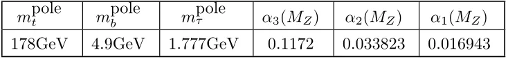
Other input parameters are shown in Table 2:

mpole_t mpole_b mpoleτ α3(MZ) α2(MZ) α1(MZ)

178GeV 4.9GeV 1.777GeV 0.1172 0.033823 0.016943

Table 2: Input parameters for the running analysis

In Table 2 the input couplings α1···3 correspond to the Standard Model MS results;

we calculate the appropriate dimensionless coupling input values for the running analysis by an iterative procedure involving the sparticle spectrum. We define gauge unification

3 _{except for the SPS6 point. The SPS6 point corresponds to non-unified gaugino masses,}

to be the scale where α2 and α1 meet; we speed up the determination of this by (at each

iteration) adjusting the unification scale using the solution of the one-loopβ-functions for the gauge couplings from the previous value of the scale. We employ one-loop radiative corrections as detailed in Ref. [24]4; thus we run up fromMZ using the full supersymmetric

β-functions. For most particles we evaluate the pole mass at a renormalisation scale equal to the pole mass itself, and determine this value by iteration; the exception being the light CP-even Higgs, where we use a scale equal to the average squark mass.

3.1. Benchmark point SPS 1a

This point is a “typical” point in MSUGRA parameter space. In Table 3 we compare our results for a selection of sparticle masses (at n5 =n10 = 0) with the spread of results

taken from Ref. [9], denoted AKP (note our convention that the predominantly right-handed top squark is ˜t2).

4 _{In the first line of Eq. 37 of Ref. [24], the first term in the square bracket should read}

−(m 2 ˜

t1+m

2 ˜

t2)B0(m˜t2, m˜t1,0): i.e. it should have a minus sign. The corresponding exact result in

mass 1loop 2loops 3loops AKP ˜

g 628 613 611 604−₆₁₂

˜

t1 594 590 583 577−588

˜

t2 400 399 391 396−401

˜

uL 573 565 557 565−569

˜

uR 552 548 539 547−549

˜_{b1 520 514 507 514}−₅₁₈

˜_{b2 551 548 540 539}−₅₄₈

˜

dL 579 571 563 571−574

˜

dR 551 548 539 546−548

˜

τ1 212 207 206 208−211

˜

τ2 139 135 135 134−136

˜

eL 209 202 202 204−207

˜

eR 147 144 144 143−146

˜

νe 192 186 185 186−191

˜

ντ 191 185 184 185−191

χ1 104 97 97 95.6−97.4

χ2 193 180 179 181−182

χ3 351 369 364 362−371

χ4 376 388 384 381−390

χ±₁ 193 179 178 180−₁₈₂

χ±₂ 376 388 384 380−₃₉₀

h 114 114 114 112−₁₁₅

H 392 403 399 403−₄₀₇

A 391 403 399 400−₄₀₆

H± _{400 412 408 410−415}

Table 3: Sparticle masses (in GeV) for the SPS1a point

3.2. Benchmark point SPS 1b

This is another “typical” point but with a higher value of tanβ. Our results are given in Table 4.

mass 1loop 2loops 3loops AKP

˜

g 967 946 943 933−₉₄₃

˜

t1 848 841 832 836−839

˜

t2 657 656 646 652−661

˜

uL 891 878 868 878−882

˜

uR 854 849 837 848−850

˜_{b1 781 773 763 773}−₇₇₈

˜_{b2 831 827 816 819}−₈₂₈

˜

dL 895 882 872 882−885

˜

dR 851 847 835 844−848

˜

τ1 353 347 346 347−349

˜

τ2 208 199 200 196−202

˜

eL 348 339 338 341−342

˜

eR 258 254 254 253−256

˜

νe 338 329 328 329−332

˜

ντ 328 318 318 319−322

χ1 173 162 162 159−163

χ2 327 305 304 308−308

χ3 507 532 526 521−534

χ4 526 546 541 534−546

χ±₁ 327 305 304 307−₃₀₈

χ±₂ 526 547 541 535−₅₄₇

h 118 118 118 117−₁₁₉

H 528 544 539 540−₅₄₄

A 529 545 540 538−₅₄₄

H± _{535 551 547 547−551}

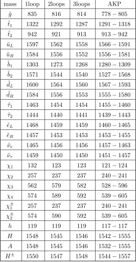
3.3. Benchmark point SPS 2

This is a “focus point region” point [25], characterised by the large value ofm0. Our

results are given in Table 5.

mass 1loop 2loops 3loops AKP

˜

g 835 816 814 778−₈₀₅

˜

t1 1322 1292 1287 1291−1318

˜

t2 942 921 913 913−942

˜

uL 1597 1562 1558 1566−1591

˜

uR 1584 1556 1552 1556−1581

˜_{b1 1303 1273 1268 1280}−₁₃₀₉

˜_{b2 1571 1544 1540 1527}−₁₅₆₈

˜

dL 1600 1564 1560 1567−1593

˜

dR 1584 1556 1553 1555−1580

˜

τ1 1463 1454 1454 1455−1460

˜

τ2 1444 1440 1441 1439−1443

˜

eL 1468 1459 1459 1460−1465

˜

eR 1457 1453 1453 1453−1455

˜

νe 1465 1456 1456 1457−1463

˜

ντ 1459 1450 1450 1451−1457

χ1 132 123 123 121−124

χ2 257 237 237 240−241

χ3 562 579 582 528−596

χ4 574 589 592 539−605

χ±₁ 257 237 237 240−₂₄₁

χ±₂ 574 590 592 539−₆₀₅

h 119 119 119 117−₁₁₇

H 1548 1545 1546 1542−₁₅₅₅

A 1548 1545 1546 1532−₁₅₅₅

H± _{1550 1547 1548 1544−1557}

3.4. Benchmark point SPS 3

This is a “co-annihilation region” point, its distinctive feature being a light stau not much heavier than the neutralino LSP. Our results are given in Table 6.

mass 1loop 2loops 3loops AKP

˜

g 964 943 940 930−₉₄₀

˜

t1 851 845 835 836−843

˜

t2 645 644 634 640−650

˜

uL 872 860 849 861−863

˜

uR 835 830 818 828−831

˜_{b1 794 787 776 786}−₇₉₃

˜_{b2 830 826 814 816}−₈₂₅

˜

dL 876 864 853 864−867

˜

dR 831 828 816 825−829

˜

τ1 300 291 290 293−294

˜

τ2 180 173 173 172−176

˜

eL 299 288 288 291−293

˜

eR 186 181 181 179−183

˜

νe 287 277 276 277−281

˜

ντ 286 276 275 276−280

χ1 172 161 161 158−162

χ2 325 302 301 305−306

χ3 512 538 531 528−540

χ4 533 554 548 543−555

χ±₁ 324 302 301 304−₃₀₆

χ±₂ 533 554 548 542−₅₅₅

h 117 118 117 116−₁₁₈

H 579 597 591 593−₆₀₀

A 579 597 591 589−₆₀₀

H± _{585 603 597 598−605}

3.5. Benchmark point SPS4

This is a point with large tanβ. Our results are given in Table 7.

mass 1loop 2loops 3loops AKP

˜

g 759 743 741 729−₇₃₈

˜

t1 705 700 693 693−697

˜

t2 544 541 533 540−544

˜

uL 777 764 757 766−772

˜

uR 755 747 739 747−751

˜_{b1 624 619 611 614}−₆₁₉

˜_{b2 693 690 683 679}−₆₉₂

˜

dL 782 769 761 770−776

˜

dR 753 746 738 746−749

˜

τ1 423 420 420 414−421

˜

τ2 272 268 268 253−269

˜

eL 455 450 449 451−452

˜

eR 419 417 418 417−419

˜

νe 447 441 441 442−445

˜

ντ 395 390 390 387−393

χ1 128 120 120 119−121

χ2 242 226 225 228−228

χ3 400 419 415 406−420

χ4 420 435 431 422−436

χ±₁ 242 226 225 227−₂₂₈

χ±₂ 421 436 432 422−₄₃₆

h 116 116 116 114−₁₁₆

H 370 386 385 355−₃₆₇

A 371 388 387 355−₃₆₇

H± _{381 397 396 366−379}

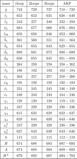
3.6. Benchmark point SPS 5

mass 1loop 2loops 3loops AKP

˜

g 743 729 727 719−₇₂₉

˜

t1 653 654 646 629−651

˜

t2 265 278 263 258−280

˜

uL 684 677 668 676−685

˜

uR 658 656 646 655−660

˜_{b1 563 563 554 554}−₅₆₇

˜_{b2 654 653 643 630}−₆₅₆

˜

dL 688 681 673 681−689

˜

dR 656 655 645 653−658

˜

τ1 264 259 258 259−262

˜

τ2 186 182 183 182−184

˜

eL 263 257 257 258−261

˜

eR 195 192 193 192−194

˜

νe 251 245 245 246−249

˜

ντ 249 243 243 244−247

χ1 128 120 120 119−120

χ2 247 229 228 230−236

χ3 608 626 621 626−631

χ4 621 637 632 637−641

χ±₁ 247 229 228 230−₂₃₆

χ±₂ 620 637 632 636−₆₄₁

h 117 118 118 116−₁₂₂

H 667 682 676 681−₆₉₄

A 667 682 677 682−₆₉₀

H± _{672 687 681 687−698}

Table 8: Sparticle masses (in GeV) for the SPS5 point withmt = 178GeV

calculated both using in Table 8 mt = 178GeV (as for the previous tables) and for

com-parison in Table 9 with mt = 174.3GeV. This illustrates the sensitivity to the input mt,

with the light stop changing over 20GeV due to this small change in mt.

mass 1loop 2loops 3loops AKP

˜

g 743 729 727 718−₇₂₈

˜

t1 652 653 645 628−649

˜

t2 243 257 240 232−258

˜

uL 684 677 668 676−684

˜

uR 658 656 646 653−660

˜_{b1 561 560 551 551}−₅₆₄

˜_{b2 654 653 643 629}−₆₅₅

˜

dL 689 681 673 680−689

˜

dR 656 655 645 651−658

˜

τ1 264 259 258 258−262

˜

τ2 186 182 182 182−184

˜

eL 263 257 257 258−260

˜

eR 195 192 192 192−194

˜

νe 251 245 245 246−249

˜

ντ 249 243 243 244−246

χ1 128 120 120 119−121

χ2 247 229 228 230−236

χ3 615 632 628 632−637

χ4 628 644 639 643−646

χ±₁ 247 229 228 230−₂₃₆

χ±₂ 627 643 639 643−₆₄₆

h 115 115 115 112−₁₁₉

H 674 688 683 687−₆₉₃

A 674 688 683 689−₆₉₃

H± _{679 692 687 694−702}

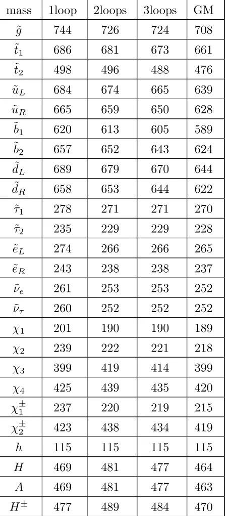
3.7. Benchmark point SPS6

mass 1loop 2loops 3loops GM ˜

g 744 726 724 708

˜

t1 686 681 673 661

˜

t2 498 496 488 476

˜

uL 684 674 665 639

˜

uR 665 659 650 628

˜_{b1 620 613 605 589}

˜_{b2 657 652 643 624}

˜

dL 689 679 670 644

˜

dR 658 653 644 622

˜

τ1 278 271 271 270

˜

τ2 235 229 229 228

˜

eL 274 266 266 265

˜

eR 243 238 238 237

˜

νe 261 253 253 252

˜

ντ 260 252 252 252

χ1 201 190 190 189

χ2 239 222 221 218

χ3 399 419 414 399

χ4 425 439 435 420

χ±₁ 237 220 219 215

χ±₂ 423 438 434 419

h 115 115 115 115

H 469 481 477 464

A 469 481 477 463

H± _{477 489 484 470}

Table 10: Sparticle masses (in GeV) for the SPS6 point

3.8. Discussion

A clear feature of the results is that the corrections due to two and three-loop running can be quite large for squarks, but are typically smaller for weakly-interacting particles. In particular the light CP-even Higgs mass is very stable. The large three-loop α3 corrections

the only MSUGRA point such that m0 > m1 2

, i.e. SPS2, the three-loop correction to the

squark masses is smaller than the two-loop one.

Generally speaking we would anticipate that for regions of parameter space where the

three-loop corrections are comparable to or exceed the two-loop ones, the four-loop ones

will be at least as large. This suggests that we are already at three loops approaching the

asymptotic region for the β-functions. So it appears that squark mass predictions with an

accuracy greater than a few per cent will not be possible using perturbation theory.

Overall our results agree reasonably well with those of existing programs [9]. One

place where we have a significant difference is for the H, A, H± _{results for SPS4. This is}

a large tanβ point; however our results for the b-squark and d-squark masses (which one

would expect to be sensitive to large tanβ) agree quite well, so for the moment we have

no explanation for this discrepancy.

4. The Semi-perturbative Region

The addition of additional matter representations in complete SU5 multiplets does

not affect gauge unification (and the unification scale) at one loop. Beyond one loop this

is no longer the case, and increasing the amount of matter relevant to the running analysis

requires the presumption of larger threshold corrections at the unification scale in order to

restore gauge unification; one is thus forced to argue that the success of gauge unification

in the MSSM is coincidental 5_.

5 _{Historically gauge unification was implemented by usingα}

3(M_Z) as an input and computing

sin2

θW, although the latter was more accurately measured, because sin

2

θW varies very slowly

with α3(M_Z), and conversely (of course) α3(M_Z) varies rapidly as a function of sin 2

θW. The

current experimental results forα3(MZ) already require us to suppose the existence ofsome high

scale radiative corrections in the MSSM; but the fact remains that things get worse as we add

0 1 2 3 4 5 6 0

0.02 0.04 0.06 0.08 0.1 0.12 0.14 0.16

α₁,α₂,α₃ vs τ for SPS1a

τ

α 1

,

α 2

,

α 3

Fig.1: Gauge coupling unification for n10 = 1.7. Solid, dashed, and dotted lines correspond to α1, α2, α3 respectively.

In Fig. 1 we show the evolution of the gauge couplings αi = gi2/(4π) for n10 = 1.7,

using three-loop β-functions for all couplings. (As remarked in Ref. [12], the mass scale of these additional multiplets being unknown it makes sense to parametrise their effects by taking n5, n10 to be continuous variables.) The couplings are plotted against τ =

1

2π ln(Q/MZ); evidently we are still in the perturbative regime. The input parameters at

MZ correspond to a typical supersymmetric mass spectrum; specifically, the Benchmark

point SPS1a. One sees clearly the need for large corrections to restore gauge unification. We gave a number of examples of the effect of additional matter on the sparticle spectrum predictions in a previous paper[15]; here we contrast the effect on the first and third generation squark masses. Thus in Fig 2 we plot, for the SPS5 point, the ratio of the ˜uL and gluino masses against n10 for n5 = 0; as already noted in Ref. [12], the mass

increases withn10. It is interesting that the effect of the three-loop correction to this ratio

where we show the behaviour of the light stop mass for the same SPS point; in this case

the ratio decreases smoothly, and the three-loop correction only cancels the two-loop one

at n10 = 0. For the SPS5 point the electroweak vacuum fails around n10 = 0.48. (The

change in this value and in Fig. 3 from our previous paper[15] is due to the change in the

input top pole mass, and to an improved treatment of the Higgs potential minimisation.)

In Fig. 4 we plot the light CP-even Higgs mass for SPS1a as a function of n10 (for

n5 = 0). We see that it is fairly stable both with respect to loop corrections and the

addition of extra matter. In the case of SPS1a the electroweak vacuum fails at around

n10 = 1.8.

0 0.05 0.1 0.15 0.2 0.25 0.3 0.35 0.4 0.45

0.91 0.92 0.93 0.94 0.95 0.96 0.97 0.98 0.99 1 1.01

u_L/gluino mass ratio vs n₁₀ for SPS5

n₁₀

uL

/gluino mass ratio

Fig.2: Plot of the u˜L/gluino mass ratio against n10 for SPS5. Solid,

dashed and dotted lines correspond to one, two and three-loop running

0 0.05 0.1 0.15 0.2 0.25 0.3 0.35 0.4 0.45 0.15

0.2 0.25 0.3 0.35 0.4

Light stop/gluino mass ratio vs n₁₀ for SPS5

n₁₀

Light stop/gluino mass ratio

Fig.3: Plot of the light stop/gluino mass ratio against n10 for SPS5. Solid, dashed and dotted lines correspond to one, two and three-loop running respectively.

0 0.2 0.4 0.6 0.8 1 1.2 1.4 1.6

113.5 114 114.5 115 115.5 116 116.5 117

Light Higgs mass vs n₁₀ for SPS1a

n₁₀

Light Higgs mass (in GeV)

5. Conclusions

We have extended typical detailed running coupling analyses for the MSUGRA MSSM SPS benchmark points to incorporate three-loop β-function corrections for the running masses and couplings. We compare our results to those obtained by existing programs using two-loop running. The spread in the results from these programs is probably due to a mixture of program errors and genuine theoretical uncertainties such as the choice of scale appropriate for the evaluation of the pole mass. Presumably over time the results used by these programs will converge; we would argue that a more reliable estimate of the ultimate theoretical error in these spectrum calculations is currently provided by the difference between our two and three-loop calculations, as opposed to the spread in the various available two-loop results.

Generally speaking the effect of the three-loop running corrections is small for weakly-interacting particles but larger for the squark masses. For the light stop mass at the SPS5 point, we see an 8% effect, but more typically the effect is between 1% and 2%. This appears to us to represent a fundamental limit on the theoretical precision of squark mass theoretical predictions.

Finally we show how additional matter inSU5 multiplets can affect the sparticle

spec-trum; more dramatically as the “semi-perturbative unification” regime [12] is approached.

Acknowledgements

References

[1] I. Jack and D.R.T. Jones Phys. Lett. B415 (1997) 383

[2] I. Jack, D.R.T. Jones and A. Pickering, Phys. Lett. B432 (1997) 114

[3] L.V. Avdeev, D.I. Kazakov and I.N. Kondrashuk, Nucl. Phys. B510 (1998) 289 [4] I. Jack, D.R.T. Jones and C.G. North, Nucl. Phys. B473 (1996) 308

[5] I. Jack, D.R.T. Jones and C.G. North, Nucl. Phys. B486 (1997) 479 [6] P.M. Ferreira, I. Jack and D.R.T. Jones, Phys. Lett. B387 (1996) 80 [7] http//www.liv.ac.uk/∼_dij/betas

[8] B.C. Allanach et al., Eur. Phys. J. C 25 (2002) 113 [9] http://kraml.home.cern.ch/kraml/comparison

[10] B.C. Allanach, S. Kraml and W. Porod, JHEP 016 (2003) 0303 [11] N. Ghodbane and H.U. Martyn, hep-ph/0201233.

[12] C.F. Kolda and J. March-Russell, Phys. Rev. D55 (1997) 4252

[13] D. Ghilencea, M. Lanzagorta and G.G. Ross, Phys. Lett. B415 (1997) 253 ; Nucl. Phys. B511 (1998) 3;

G. Amelino-Camelia, D. Ghilencea and G.G. Ross, Nucl. Phys. B528 (1998) 35 [14] B. Brahmachari, U. Sarkar and K. Sridhar, Mod. Phys. Lett. A 8 (1993) 3349;

R. Hempfling, Phys. Lett. B351 (1995) 206;

K.S. Babu and J.C. Pati, Phys. Lett. B384 (1996) 140

[15] I. Jack, D.R.T. Jones and A.F. Kord, Phys. Lett. B579 (2004) 180 [16] I. Jack, D.R.T. Jones and R. Wild, Phys. Lett. B509 131 (2001)

[17] I. Jack, D.R.T Jones, S.P. Martin, M.T. Vaughn and Y. Yamada, Phys. Rev. D 50, 5481 (1994)

[18] D.R.T. Jones, Phys. Lett. B123 (1983) 45 ; V. Novikov et al, Nucl. Phys. B229 (1983) 381 ; V. Novikov et al, Phys. Lett. B166 (1986) 329 ;

M. Shifman and A. Vainstein, Nucl. Phys. B277 (1986) 456

[19] I. Jack, D.R.T. Jones and A. Pickering, Phys. Lett. B432 (1998) 114 [20] W. Siegel, Phys. Lett. B84 (1979) 193;

D.M. Capper, D.R.T. Jones and P. van Nieuwenhuizen, Nucl. Phys.B167 (1980) 479 [21] J.E. Bj¨orkman and D.R.T. Jones, Nucl. Phys. B259 (1985) 533

[22] D.I. Kazakov, hep-ph/0208200

[23] I. Jack and D.R.T. Jones, Phys. Lett. B473 (2000) 102;

I. Jack, D.R.T. Jones and S. Parsons, Phys. Rev. D62 (2000) 125022; I. Jack and D.R.T. Jones, Phys. Rev. D63 (2001) 075010