This is a repository copy of
On the development of time period and mode choice models
for use in large scale modelling forecasting systems
.
White Rose Research Online URL for this paper:
http://eprints.whiterose.ac.uk/43610/
Article:
Hess, S, Daly, AJ, Rohr, C et al. (1 more author) (2007) On the development of time period
and mode choice models for use in large scale modelling forecasting systems.
Transporation Research Part A: Policy & Practice, 41 (9). 802 - 826 . ISSN 0965-8564
https://doi.org/10.1016/j.tra.2007.04.001
eprints@whiterose.ac.uk https://eprints.whiterose.ac.uk/ Reuse
Unless indicated otherwise, fulltext items are protected by copyright with all rights reserved. The copyright exception in section 29 of the Copyright, Designs and Patents Act 1988 allows the making of a single copy solely for the purpose of non-commercial research or private study within the limits of fair dealing. The publisher or other rights-holder may allow further reproduction and re-use of this version - refer to the White Rose Research Online record for this item. Where records identify the publisher as the copyright holder, users can verify any specific terms of use on the publisher’s website.
Takedown
If you consider content in White Rose Research Online to be in breach of UK law, please notify us by
On the development of time period and mode choice models for use in large
scale modelling forecasting systems
Stephane Hess Imperial College London
stephane.hess@imperial.ac.uk
Andrew Daly RAND Europe
daly@rand.org
Charlene Rohr RAND Europe
crohr@rand.org
Geoff Hyman
UK Department for Transport
geoff.hyman@dft.gsi.gov.uk
The opinions expressed in this paper are those of the authors and do not necessarily represent the views or policies of the UK Department for Transport.
ABSTRACT
A substantial amount of research is presently being carried out to understand the complexities involved in modelling the choice of departure time and mode of travel. Many of these models tend to be far too complex and far too data intensive to be of use for application in large scale model forecasting systems, where socio-economic detail is limited and detailed scheduling information is rarely available in the model implementation structure. Therefore, these models generally work on the basis of a set of mutually exclusive time periods, rather than making use of continuous departure time information. Two important questions need to be addressed in the use of such models, namely the specification used for the time periods (in terms of length), and the ordering of the levels of nesting, representing the difference in the sensitivities to shifts in departure time and changes in the mode of travel. This paper aims to provide some answers to these two questions on the basis of an extensive analysis making use of three separate Stated Preference (SP) datasets, collected in the United Kingdom and in the Netherlands. In the analysis, it has proved possible to develop models which allow reasonably sound predictions to be made of these choices. With a few exceptions, the results show higher substitution between alternative time periods than between alternative modes. Furthermore, the results show that the degree of substitution between time periods is reduced when making use of a more coarse specification of the time periods. These results are intended for use by practitioners, and form an important part of the evidence base supporting the UK Department for Transport’s advice for practical UK studies in the WebTAG system1.
1. INTRODUCTION
As a result of increasing road congestion and road pricing, modelling the temporal response of travellers to transport policy interventions has rapidly emerged as a major issue in many practical transport planning studies. A substantial amount of research is therefore being carried out to understand the complexities involved in modelling time of day choice. These models are contributing substantially to our understanding of how travellers make time-of-day decisions (cf. de Jong et al., 2003; Hess et al., 2006).
The resulting models, however, tend to be far too complex and far too data intensive to be of use for application in large scale model forecasting systems, where socio-economic detail is limited and detailed scheduling information is rarely available in the model implementation structure. As such, while detailed modelling applications work with continuous departure and arrival time information, large scale forecasting systems work with the concept of time periods, where the continuous time space is aggregated into a finite number of mutually exclusive time periods. Examples range from Domencich & McFadden (1975) to RAND Europe (2005a).
Another difference between small scale analyses and large scale model forecasting systems comes in the choice of model structure, i.e. the actual modelling methodology rather than the structure of the choice set (continuous vs discrete). Indeed, with the significant advances made in the field of discrete choice modelling over the past decade (cf. Train, 2003), analysts now have at their disposal a methodological toolbox that allows for an ever more realistic representation of complex real world choice processes. This is especially true in the context of the Mixed Multinomial Logit (MMNL) model (cf. McFadden & Train, 2000), which allows for a representation of random taste heterogeneity across respondents. The flexibility of these random coefficients models however comes at the cost of a computationally far more expensive estimation and application process, due to the reliance on numerical simulation. While acceptable in small scale studies, this reliance on computer-intensive simulation in both estimation and application makes these models generally inapplicable in practical planning, where the computer run times implied are simply too long. For example, initial estimates for the PRISM system in the West Midlands suggest MMNL run times for forecasting in excess of 100 days!
On the basis of the above two observations, the aim of this paper is therefore to describe the development of time period (TP) choice models which are suitable for application in large scale modelling forecasting systems, such as those widely used in Europe today (e.g. RAND Europe, 2005a).
Two main issues need to be addressed in the development of an appropriate model specification. The first relates to the specification of the time periods used in the analysis, i.e. the method that is used in aggregating continuous departure times into a set of mutually exclusive subsets. Essentially, this reduces to a decision as to how many time periods are to be used in the analysis, and where each given time period begins and ends (thus determining time period length). By varying the size of the time periods, modellers can answer questions as to the relationship between the choice probabilities of different time periods, such as for example whether the elasticity for shorter shifts is greater than that for longer shifts.
The second main issue that needs to be addressed is that of model structure. As described above, for reasons of computational cost, random coefficients structures are inapplicable, such that attempts need to be made to represent all taste heterogeneity in a deterministic fashion. Here, even the most basic model structure, the Multinomial Logit (MNL) model, would suffice. However, with the specific nature of the now imposed choice set, i.e. the aggregation into mutually exclusive time periods, it becomes likely that alternatives belonging to the same time period share unobserved attributes, leading to correlated errors, a phenomenon that cannot be represented by the MNL model. This correlation can however be represented with the help of Generalised Extreme Value (GEV) models, such as the Ordered GEV (OGEV) model (Small, 1987) or the Nested Logit (NL) model (Daly & Zachary, 1978, McFadden, 1978, and Williams, 1977), which, like MNL, have an analytical solution, hence not leading to a requirement for using simulation.
A further complication arises in the choice of model structure. Indeed, large-scale practical planning models typically represent choices along multiple dimensions at the same time, such as for example the joint choice of departure time and mode of travel. This means that a multi-level model structure is now required. Here, the main question that needs to be addressed is the position of each choice relative to other choices, where, in the present context, this equates to the choice of a structure nesting mode choice above or below the choice of a time period.
studies undertaken over the past 15 years in the United Kingdom and the Netherlands specifically to address these issues2.
The remainder of this paper is organised as follows. The next section describes the data used in the analysis. This is followed in Section 3 by a description of the modelling methodology used, in terms of model structure as well as specification of the utility functions. Section 4 discusses the results of the analysis and Section 5 presents a brief forecasting example. Finally, Section 6 presents the conclusions of the research.
2. DATA SOURCES
The models discussed in this paper are developed from data collected for three studies of mode and time of day choice. Each of these data collection exercises formed part of larger urban, regional or national model development projects. These are, in chronological order of the collection date: the APRIL model for London (Bates & Williams, 1993; Polak & Jones, 1994), work in The Netherlands (de Jong et al., 2003) and the PRISM model developed for the West Midlands region of the United Kingdom (RAND Europe, 2004). In the remainder of this paper, these three datasets will be referred to respectively as the APRIL, Dutch and PRISM datasets.
All three datasets were collected through Stated Preference (SP) surveys which shared a number of important features:
• All three surveys concentrated principally on the re-timing and/or mode switching of travellers making observed car journeys, although the Dutch survey also collected data on re-timing and mode switching from travellers making train journeys. A motivating policy interest in all three studies was the potential response of travellers to road user charging initiatives, so this issue was tested directly in the stated preference scenarios.
• In all the surveys, the travel alternatives were presented to respondents in the form of complete tours, such that the influence of congestion or road pricing was evaluated in terms of both the respondent’s outward and return journey and the time they would spend at their destination. The Dutch and PRISM studies also investigated departure time responses for non-home-based business trips; the analysis of these one-way journeys differs from other journeys through the absence of a choice of return time period.
• In each survey, the main travel purposes distinguished were commuting, business and other. • All studies included an option to not travel.
The APRIL dataset was collected in 1992 from a sample of approximately 1,000 car drivers contacted at various locations in inner and outer London. Respondents were presented with a series of choices, each between two alternatives with varying departure time and road pricing characteristics. An illustration of the format of the SP choice experiment used in the survey is given in Figure 1.
The Dutch data was collected in 2000 from a sample of approximately 1,000 travellers, contacted at a selection of sites across The Netherlands, concentrating on areas where road and rail congestion was encountered in peak-period journeys. Both car drivers and train users were interviewed in the Dutch survey. Respondents were presented with a series of choices offering three departure time alternatives: a “peak” alternative, which was close to the observed/preferred departure time for their observed mode of travel, a considerably “earlier” alternative and a considerably “later” alternative. An alternative mode, with varying characteristics, was also presented to respondents who indicated that an alternative mode existed for their journey.
2 The work described here was largely performed in a study carried out by RAND Europe and Imperial
The PRISM dataset was collected in 2003 from a sample of over 550 car drivers undertaking journeys entirely within the West Midlands county in the UK. The SP design and presentation was virtually identical to the Dutch study, apart from the fact that only car drivers were interviewed. An example screen from the PRISM study is shown in Figure 2.
Although detailed differences exist amongst these datasets (including in respect of the associated socio-demographic information collected), there is an unusually high level of consistency in the treatment of key SP design features. This provided an excellent opportunity to undertake a comparative analysis of the mode and time of day substitution patterns in these datasets using similar model forms, whilst minimising concerns regarding the potential confounding influence of differences in the data collection process.
3. MODELLING ANALYSIS
Two different modelling approaches were used in the study to gain insight into travellers’ departure time choice, and these will now be looked at in turn.
3.1. Models using continuous departure time information
Prior to the analysis using time period models, which is the main topic of this paper, a set of continuous departure time models were estimated from the SP data. Like the time period models, these models describe an alternative in terms of its travel time and travel cost. However, while in the time period models, the scheduling information is incorporated through allocation of alternatives into mutually exclusive subsets, this first set of models makes use of schedule delay information, given by the difference (in continuous time space) between the scheduled and preferred departure/arrival times.
One of the main aims of this study was to gauge the relative sensitivity of shifts in departure time and changes of mode. In the context of the time period models presented later in this paper, this is done with the help of multi-level NL models that nest time period choice above or below mode choice. A nesting approach is not applicable in the case of a continuous departure time model, as there is no predetermined structure for grouping together alternatives by departure time. To overcome this difficulty, normally distributed error-component terms are added to the utility function, moving from a MNL specification to an error-components formulation of the MMNL model (cf. Train, 2003).
The utility function used in the MMNL model differs from that of the basic Multinomial Logit (MNL) model through the presence of an additional error component ηi, such that the utility for alternative i is given by:
Ui = Vi + ηi + εi, [1]
where Vi gives the observed part of the utility of alternative i, and εi, is assumed to follow a Gumbel
distribution, independent across alternatives and observations (cf. Train, 2003, which also reviews the original literature).
In the present work, the MMNL models were estimated on the continuous SP data, and the observed part of utility Vi captures respondents’ sensitivities to changes in attributes presented in the SP survey, such
as travel time, travel cost, and indeed schedule delay, measured as the difference between the actual and preferred arrival times. As indicated above, the additional error components ηi are used to test for the
differences in the relative sensitivities to changes in departure time and mode of travel, allowing us to gauge the shift in departure time that is required before a change of mode becomes more attractive, all else being equal. Specifically, the formulation from equation [1] is adapted such that we have:
Ui = Vi + E· 1·EDEP(i) + L· 2·LDEP(i) + M· 3·MODECHANGE(i) + εi, [2]
where 1, 2 and 3 are random variates drawn independently from the standard Normal distribution, and E, L, and M are the standard deviations of the error components.
while in the Dutch and West Midlands models, the shift was relative to the departure time in the base alternative (such that EDEP=0 for the “retimed late” alternative, and LDEP=0 for the “retimed early” alternative, with both being equal to zero for the base alternative):
EDEP(i) = max ( 0, (reference departure time) – (presented departure time) ) [3] LDEP(i) = max ( 0, (presented departure time) – (reference departure time) ) [4] In each case, the utility of an alternative i contains at most one of the three error components from equation [2]3, where, due to the multiplication by EDEP(i) and LDEP(i) respectively, the variances of the error components are thus proportional to the extent of the shift in departure time from the reference departure time.
The relative magnitude of the estimated variances of the error components associated with the mode and time of day dimensions provide a measure of the relative sensitivity of these two dimensions to changes in the substantive (i.e. observed) attributes of travel (with smaller variances of the error components implying, ceteris paribus, higher sensitivity). As such:
• the significance and magnitude of E and L indicate the significance and magnitude of
heteroskedasticity between time shift alternatives as a function of the size of the shift in time; and • the relative values of E and L indicate whether earlier or later shifting is more sensitive;
the relative value of M to E and L (together with the size of time shifts) indicates the relative sensitivity of
mode choice to time choice; thus if M is larger than E and L, when the latter are multiplied by a given time
shift, then we may conclude that, for time shifts of up to that size, mode choice is less sensitive to explanatory variables than is time shifting (owing to the larger variance of the error term).
MMNL models using the above specification were estimated on all three datasets, across the various purpose segments. The findings of this analysis are described in detail by Hess et al. (2006). That analysis shows that very good performance was obtained for the models using the Dutch and PRISM data. On the other hand, it was not generally possible to estimate significant error components for either mode or time shifts with the APRIL data.
The results from this analysis are most readily summarised by looking at the ratios between the error components associated with mode changes and time shifts, as shown in Table 1. These show the shift in departure time required for the sensitivity (to explanatory variables) of mode choice to be as high as the sensitivity of the choice of departure time. Given the lengths of time periods generally considered in large scale modelling work (usually 2-3 hours), the results show that, across the two data sets, and across purposes, travellers are more likely to accept a shift in departure time than a change of mode. The only exception to this comes in the form of shifts to a later departure time for commuters with inflexible work hours, where a later time shift of more than 47 minutes (or an earlier time shift of more than 108 minutes) would indicate a greater sensitivity for mode shifting than for time shifting; that is, faced with time shifts of this magnitude (and always with the reservation of ceteris paribus), equal numbers would shift time and change mode.
3.2. Development of Time Period Models
From the above discussion, it should be clear that the specification in Section 3.1 makes extensive use of disaggregate information regarding the characteristics of existing travel (e.g., via the shift variables EDEP and LDEP), obtained from the SP sample. As such, a number of continuous variables enter the model: travel time, travel cost, and schedule delay. The last especially causes significant problems in the case of large scale model systems, where detailed socio-demographic information relating to preferred or current departure times is not generally available, preventing the calculation of schedule delay measures. This leads to a need for a different modelling approach, free from the requirement to have schedule delay information as an input, which in turn leads to the use of models where continuous departure times are aggregated into mutually exclusive time periods.
3
Another issue with the approach from Section 3.1., which uses error components to measure the relative sensitivities to departure time and mode changes, is that the reliance on simulation both in estimation and application would make its use in large scale model systems prohibitively expensive. Indeed, while the added cost may be acceptable when estimating only a handful of models on small samples (as in the analysis of Hess et al., 2006), this is no longer the case when having to apply the models in practical studies, where a large number of application runs will be required to gauge the changes in different hypothetical scenarios. This issue of the higher computational cost can be addressed by making use of model structures from the GEV family whose choice probabilities are given in a closed form expression, while still allowing for the flexible error structure used in the error components models.
Before proceeding with a detailed description of the modelling methodology, it should be acknowledged that moving from continuous departure time models to time period models almost inevitably leads to a drop in model performance and hence forecasting accuracy. However, this is unavoidable, as the more detailed models are inapplicable in large scale model systems. As such, the models presented in this paper should not be seen as state-of-the-art discrete choice methodology, but rather as the best possible approach to be used in actual large scale policy-oriented studies. This is not only an indication of the gap between the state-of-the-art and the state-of-practice, but also an illustration of the limitations imposed on actual modelling analyses by the requirements of advanced model structures in terms of data and computational cost. Here, it should be noted that the move from MMNL models (in the continuous case) to GEV structures (in the time period models) is in this case exclusively motivated by computational issues, and, in the absence of a treatment of random taste heterogeneity, there is no loss in flexibility as GEV structures are able to deal with the correlation between alternatives sharing the same mode of travel or being closer to each other in terms of departure time.
3.2.1. Converting the SP Data to Discrete Alternatives
This section looks at the process used in the association of continuous departure times with different time periods. To allow us to examine the differences in sensitivity for differently sized time periods (and hence shifts in departure time), three different aggregation procedures were used, grouping the 24-hour continuum into:
• twenty-four one-hour periods; • five coarse time periods; and
• sixteen 15-minute morning-peak periods, and two coarse pre-peak and post-peak periods (for commuter models only).
The specification of the time periods is the same across datasets in the case of the one-hour approach and the 15-minute approach. In the former, we have 24 time periods of a length of 60 minutes, while in the latter, we have sixteen time periods of a length of 15 minutes during the morning peak (between 6AM and 10AM), along with two coarse time periods used to complete the day’s 24 hours, one running from midnight to 6AM, and one running from 10AM to midnight4. In the coarse models, which divide a day into 5 separate periods, giving a morning peak and off-peak, an afternoon peak and off-peak, and an inter-peak period, the actual specification of the time periods differs slightly across the three datasets used (for reasons of SP design and local planning practice), as shown in Table 2.
A question now arises as to whether to allocate journeys to time periods on the basis of the journey departure time, the arrival time, or some intermediate time. The decision was taken to allocate journeys to time periods on the basis of the journey departure time, mainly because of the requirements of the forecasting systems for which the models were developed. Further complexity is introduced with the
4The main interest of these models was in the representation of detailed time period choice for commuters’
consideration of the simultaneous choice of both the outward and return period in modelling time period choice for a tour. This is accommodated by defining the time period alternatives as combinations of outward and return periods – e.g. [06:00-06:59, 19:00-19:59]. In the case of five time periods, we have 15 outward and return time period choice alternatives (N(N+1)/2), assuming that the return journey leg occurs after the outward leg, i.e. in the same period or later. In the case of 24 one-hour time periods, this increases to 300 outward and return time period combinations. The time period specification of the non-home-based trips models is much simpler because only the time period choice for one leg is modelled (N alternatives). The same applies for the 15-minute models, where again, only the outbound journey is modelled.
3.2.2. Correlation structure
As mentioned in the introduction, it is important to allow for correlation between alternatives that are close to each other in departure time or alternatives that share the same mode of travel. In the present analysis, this was done with the help of structures belonging to the family of Generalised Extreme Value (GEV) models. While models such as OGEV and other advanced nesting structures can allow for closer correlations of alternatives closer in time, it had been found in previous work on the Dutch data that these were complicated and did not give very large improvements; moreover, the aim of simplicity required for practical implementation pointed strongly to the use of simple Nested Logit (NL) models (McFadden, 1981; Daly, 1987) with all the time period alternatives presented as parallel choices. With the aim of analysing the relative sensitivity to changes in departure time and mode, two different tree structures were explored, nesting mode above time period, i.e. testing for higher sensitivity in time period choice relative to mode choice, and nesting time period above mode choice, testing the alternative structure.
The two nesting structures are illustrated in the diagrams in Figures 3 and 4 for the Dutch and PRISM data, showing the tree structures with mode above time period, and time period above mode respectively. Slight differences arise in the case of the APRIL data, as described later in this section. In the models nesting mode above time period choice, the nesting parameter tpchoice is associated with the nests containing the composite alternatives that share the same mode, while in the models nesting time period above mode, the nesting parameter modescale is associated with the nests containing the composite alternatives that share the same time period.
Independently of the nesting structure, 4 SP choice alternatives appear below each time period combination nest, leading to a 60-alternative model for the analysis of the 5 coarse time periods and a 1200-alternative model for the analysis of the one-hour time period model. However, for any one observation, only 4 elemental alternatives are available, i.e. those that were presented in the SP choice observations. For this reason, the great majority of the time periods are treated as unavailable for a given SP observation, since there are no elementary alternatives which are allocated to those time periods. Nevertheless, especially when using a more coarse specification of the time periods, it is clearly possible for more than one SP alternative to fall into the same time period nest, where, in conjunction with the nesting by mode, a maximum of three alternatives can fall into a single lower-level nest (three car alternatives falling into the same time period). This complication was accommodated by specifying a third level in the tree, containing nests that are linked to a specific time period and a specific mode. These nests use the structural parameter SPchscale, associated with the correlation between SP alternatives within the same mode and time period. This in effect only applies to car alternatives, given that only a single public transport (PT) alternative was ever included in a given SP experiment (the Dutch data from public transport users was not analysed in the present work).
Finally, each of the resulting alternatives is linked to the elementary alternative via a dummy layer with the SPscale parameter. While this is treated in the estimation as a structural parameter, it in fact plays a rescaling role, as discussed in the next section, and can be ignored from the point of view of understanding the hierarchical structure.
non-home-based business trip models in the Dutch and PRISM datasets contain only time period alternatives defined by departure time, with the same applying for all 15-minute models. Joint models based on the home-based business tours and non-home-based business trips were also developed, pooling both the tour and trip datasets, with appropriate tree structures for the tour and trip components.
A further point needs to be addressed at this stage. It is theoretically possible to allow for a different nesting structure across time periods, such that for example, with alternatives nearer the observed/preferred departure time, the choice of time period is nested below the choice of mode, with the opposite applying for alternatives further from the observed/preferred departure time. However, not only is it difficult to find a clear basis for such an approach, but the number of different possibilities is very high, when for example thinking about what constitutes a significant difference from the observed/preferred departure time. For these reasons, and for simplicity, the decision was taken to model all time period alternatives at the same level in the hierarchy.
Before passing on to the discussion of the specification of the utility functions, it is worth briefly looking at the choice of NL models as the structure used in the present analysis. Indeed, it would clearly have been possible to express the correlation structure with the help of an error components formulation of the MMNL model. With that approach, an error component would have been associated either with the three car alternatives or with the single public transport alternatives, to account for the within-mode correlation. Similarly, a separate error component would have been associated with each outbound time period, each return time period and each possible duration, hence allowing us to capture correlation between alternatives sharing the same time periods. In practice, the computational cost associated with such a model does however give the NL approach a very significant advantage over the MMNL model in the present context. This discussion also illustrates that the choice of a GEV or MMNL structure is not pre-determined by the use of a time period or continuous departure time specification. In fact, the opposite applies, where the use of a time period specification in fact facilitates the use of a GEV structure.
3.2.3. Specification of Utility
We now turn our attention to the specification of the utilities in the time period models. In each of the models, four groups of parameters were included in the utility functions. These are:
• marginal utilities of travel time and travel cost, • socio-demographic dummy variables,
• time period constants, and • alternative-specific constants.
A major problem with time period models is that of the marginal utility coefficients to be used for travel time, and by extension (due to correlation), travel cost. Due to aggregation of the data into time periods, and the accompanying loss of detail in the data, it is often not possible to estimate adequate coefficients for the relative marginal values of the utility components. This is even more so the case when the time period models work on the basis of period averages for the calculation of travel times. As such, these models generally make use of prior parameters, obtained either from the relevant literature or generated through estimation work on related continuous time data. The latter is the case in the present analysis, where the relative parameter estimates from the continuous departure time models (cf. Section 3.1) are used as priors in the estimation of the time period models, and where the decision to use additional segmentation within purpose groups (e.g. by income or by mode) was dependent on results of the continuous departure time analysis (cf. Hess et al., 2006).
other than travel time and travel cost were included in the model, based on the reasoning that additional scheduling information is usually not available in large scale forecasting models.
An important point that should be stressed here is that it is only the relative values of the utility components, e.g. the ‘values of time’, that are imported. The key coefficients giving the sensitivity of travellers to overall utility, which in turn indicate the scales in the model and hence the appropriate structures, are estimated in the NL models. The success of the procedure of importing relative values can be tested by looking at the significance in the estimated models of the compound utility components created using these imported coefficients, i.e. the parameters of the nesting structures.
The second group of parameters in the above list includes terms showing the effect of low education, age and sex on the attractiveness of the different alternatives, although some of the models do not contain any socio-demographic parameters.
In the absence of scheduling coefficients relating to preferred timings (see above), the aggregate scheduling information in time period models is generally captured through the use of a set of constants, associated with the different time periods. In effect, these constants can be seen as a more flexible specification of alternative-specific constants, capturing the mean of the unobserved part of utility associated with a specific time period, or combination of outbound and return time period. For a study of different ways of specifying these constants, see Hess et al. (2005). In the context of this analysis, an optimal specification would use a separate constant for each possible combination of outbound and return time period (with one value fixed to ensure identification), hence indirectly also capturing activity duration. However, with N separate time periods, we have N(N+1)/2 time period pairs, for which N(N+1)/2-1 pair-specific constants could be estimated. For a model with 24 one-hour time periods, this thus leads to a total of 299 constants to be estimated, in addition to the mode specific constant, any SP-related alternative specific constants and dummy variables.
This number increases quadratically with finer specifications of the time periods, rapidly leading to problems. Indeed, not only is the computational cost of this approach very high, but important issues of identification can also arise. A number of constants will invariably tend to minus infinity, as the associated time period combination is never chosen even though it is included in a number of choice sets. The converse problem, with constants tending to plus infinity, occurs in the case of combinations that are always chosen when available. In the former case, the problem can be resolved by making the associated alternatives unavailable, while in the latter case, the associated observations need to be excluded. While the former approach has no effect on model estimation (given that the associated choice-probabilities are now zero, instead of arbitrarily close to zero), the latter approach results in a reduction in the sample size and eliminates valuable information. Finally, a potentially large number of constants will simply be equal to zero (no information, i.e. never presented), or be insignificantly different from zero (very little information).
An alternative approach consists of the use of two separate sets of constants for outbound and return time periods. However, since the constants have no inherent ordering, this approach means that any information on activity duration is lost. It therefore becomes advisable to use an additional set of constants representing this duration, which can be calculated as the difference between the arrival period on the outbound leg, and the departure period on the return leg. In the one-hour example, this thus leads to three sets of 24 constants, where 23 constants are estimated in each set (departure, arrival and duration). This leads to a reduction in the (maximum) number of estimated constants from 299 to 69. However, some problems with identification can remain, as not all constants take on finite values, for the same reasons described above. In this case, further availability conditions need to be applied to make the affected alternatives unavailable, resulting in reduced choice sets and/or sample sizes. An alternative approach would be to use a functional form for the time period constants, as described by Hess et al. (2005); this is however beyond the scope of the present analysis, as it poses additional complications of specification, identification and estimation and is therefore not suitable in the present context aimed at developing models usable in practice.
The specification of the time period constants is dependent on the definition of the time periods used. Formally, in the one-hour models for car tours, three sets of constants were tested:
• a constant identifying the activity duration in terms of time periods.
In the non-home-based trip models, only the first constant was used. This was also the case for the 15-minute models for commuters, where the focus was primarily on the outbound leg. In the coarse time period models, the optimal approach of using constants linked to outbound-return pairs could be used, since there were relatively few time period combinations. Also, the unequal length of the time periods makes the use of duration constants inappropriate. Hence a single constant was included in the utility function of each alternative, defining the combination of outbound period and return period. In all three approaches, a base period (or period combination) needs to be specified for each set of constants, for reasons of identification.
While the models defined by this process contain a large number of constants, they remain suitable for their purpose of estimating changes in departure time choice resulting from changes in the time or cost of alternatives, since the effect of the constants is to put the time and cost changes into the appropriate base context. In the current study, the interest is largely in the structural coefficients, i.e. the scales, and again a correct set of constants is necessary to estimate these coefficients in the proper context, given that the constants bring the mean of the unobserved part of utility to zero. Essentially, the constants give the preference for timing options averaged over the population, and we have little a priori information on these preferences (no scheduling information in aggregate models), so that their representation by estimated constants is essential and the best approach. It is clearly not reasonable to assume that the preference for one period is the same as for another, which would be the requirement to eliminate the constants.
The final element in the utility specification relates to the alternative specific constants, which include:
• a mode specific constant for public transport, which was used in all models,
• an early-departure constant, applicable to the earlier departure time alternative in the SP exercise used in the West Midlands and Dutch models, and
• a late-departure constant applicable to the later departure time alternative in the SP exercise, used in the West Midlands and Dutch models.
The last two constants are referred to as SP rescheduling constants. It is not clear a priori whether these constants capture real preferences for the chosen time period or whether they are artefacts of the stated preference exercise, like SP inertia terms. Models were therefore tested both with and without these rescheduling constants. In each set of models estimated, the inclusion of the two constants led to very significant gains in model fit. Furthermore, and crucially, without the inclusion of these constants, no correlation along the mode choice or time period choice-dimension can be identified, so that the preferred structure is always MNL. Finally, in some of the models, the inclusion of the constants is a prerequisite for model estimation, with models not including the constants failing to converge. Even though this discussion does not clarify whether the constants capture rescheduling behaviour or SP design effects, or both, it is clear that their inclusion is very beneficial to model performance. As such, the recommended models for the PRISM and Dutch data include these additional rescheduling constants, and results for models estimated without these constants are not reported here (see RAND Europe, 2005a). Even assuming that these constants do to some degree capture scheduling behaviour, they would not be included in a forecasting model, where no scheduling information would be available. Nevertheless, they are crucial in the estimation of the remaining model parameters that would be included in such a forecasting system.
Summarising, formally, in the most general case, the utility of alternative i is defined as follows:
U(i) = SPscale ·
[ ∑j TTC,j· j·TTC + ∑j TCC,j· j·TCC + ∑j TTPT,j· j·TTPT + ∑j TCPT,j· j·TCPT {travel variables*socioeconomic variables – β fixed from MMNL models}
+ early· i,early + late· i,late + PT· i,PT + ∑j i,j· j ]
+ ∑k=1,…,K out(k) · i,out(k)
{1 hr/15 min time period constants –outward(trip and tour) }
+ ∑l=1,…,L ret(l) · i,ret(l) + ∑m=1,…,M duration(m)· i,duration(m)
{1 hr (tour) time period constants – return and durations (tours only)}
+ ∑k=1,…,K ( ∑l=1,…,L ( out(k), ret(l) ·[ i,out(k) · i,ret(l)]) )
{coarse (tour) time period constants – outward & return combinations (tours only)},
where the rescaling by SPscale applies only to the non-composite part of the utility functions, and where: TTC = travel-time for car
TCC = travel-cost for car
TTPT = travel-time for public transport TCPT = travel-cost for public transport
j = indicator variable for socio-demographic group j TTC,j = marginal utility of car time for group j
TTPT,j = marginal utility of public transport time for group j TCC,j = marginal utility of car cost for group j
TCPT,j = marginal utility of public transport cost for j early = SP constant for early departure
late = SP constant for late departure PT = constant for public transport
i,early = indicator variable for early departure for alternative i, always 0 in London models i,late = indicator variable for late departure for alternative i, always 0 in London models i,PT = indicator variable for public transport for alternative i
i,j = socio-demographic constant for alternative i and group j
i,out(k) = indicator variable for outbound departure in period k for alternative i i,return(l)= indicator variable for return departure in period l for alternative i out(k) = constant for outbound departure in period k
return(l)= constant for return departure in period l
i,duration(m) = indicator variable for duration of m periods for alternative i duration(m) = constant for duration of m periods
out(k), return(l) = constant for outbound departure in period k and return departure in period l
With this notation, out(k) is set to zero for all k in the coarse models; return(l) and duration(m) are set to zero for
all l and m respectively in the coarse models, all non-home-based trip models, and the 15-minute models; and out(k), return(l) is set to zero for all k and l in all models except the coarse models.
Other than the relative time and cost coefficients, all remaining parameters were estimated directly from the data in the time period choice models.
4. TIME PERIOD MODEL RESULTS
between 0 and 1). Additionally, in some cases, constraints are required for all structural parameters5, such that the concerned NL model reduces to MNL.
Given the wealth of models estimated on the data, it is impossible to present all the results in this paper. For this reason, we present detailed results for a single example, namely the models for commuters in the PRISM data, with summary results given for other combinations of datasets, purposes and time period specification. Detailed results for all models are given in RAND Europe (2005a).
4.1. Detailed results for PRISM commuters
The presentation of the detailed results for the three types of time period models estimated for commuters in the PRISM data starts with the one hour models, before moving on to the coarse models and the 15-minute models.
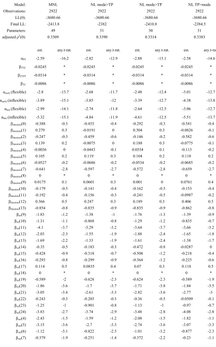
As not all time period constants can be estimated for reasons of identification, it is necessary to use some form of normalisation. In the one hour models, one constant along each dimension was therefore constrained to zero, namely the constants for the 8th outbound period (i.e. departure between 7AM and 8AM), the 18th return time period (i.e. return departure between 5PM and 6PM), and the constant equating to a duration between 7 and 8 hours. Three different models were estimated, a basic MNL model, a NL model nesting mode choice above time period choice, and a NL model nesting time period choice above mode choice. The results of this estimation process are summarised in Table 3, in which, for the nesting parameters, the asymptotic t-ratios are calculated with respect to the difference of the coefficient from 1 instead of 0.
As discussed in Section 3.2.3, the marginal utility coefficients β for travel time and travel cost were imported from the continuous MMNL models, where the parameter SPscale ensures a scale correction. In addition to the various time period constants, constants were estimated for the PT alternative, the early departure alternative and the late departure alternative. For the rescheduling constants, separate values were estimated for commuters with flexible and inflexible working hours. The results show higher reluctance by commuters with inflexible working hours to shift to earlier and later departures, which was to be expected. The high levels of statistical significance for the four rescheduling constants are an indication of the importance of including this information in models of time of day choice. For the three sets of time period constants, only those included in the final model specification are shown in Table 3, where constants causing problems were not included in the model, using the approach described in Section 3.2.3. Here, it should be noted that a large number of constants are not significantly different from zero; this is mainly a result of the small number of times that these time periods were included in the choice sets. Similar issues can arise in the case of alternative specific constants with large choice sets.
In terms of structural conclusions, we can see that, in both NL models, the SPchscale parameter is greater than 1, where, for the model nesting time period choice above mode choice, the modescale parameter also takes on an unacceptable value, making this latter model unacceptable. When constraining the
SPchscale parameter to 1 in the model nesting mode choice above time period choice, a valid tpchoice
parameter is obtained, and while the model offers only a relatively small improvement in model fit over the MNL model (by 3 units), these results do suggest that a structure nesting time period choice below mode choice is supported by the data.
In the models using the coarse time period definition, the constant associated with an outbound departure in the second time period and a return departure in the fourth time period was normalised to zero. Due to the use of a different time period formulation, slightly fewer observations had to be excluded for identification reasons in the coarse models, leading to an increase from 2,922 observations to 2,929. The results for commuters are shown in Table 4. The use of the coarse time period specification leads to a slightly poorer model fit, on the basis of the adjusted 2 measure6, while the various alternative specific constants again all attain high levels of statistical significance. Although the model using nesting of mode above TP is acceptable with a constraint on SPchscale, the estimate of tpchoice is not significantly different
5 This excludes , for which the range condition does not apply, as discussed in Section 3.2.3.
6
from 1, and the improvement in log-likelihood over the MNL model is not significant. With the model nesting time period choice above mode choice producing unacceptable values for both nesting parameters, MNL remains the preferred structure. This suggests that, with the coarse time period specification, it is not possible to establish a difference in the sensitivities along the mode choice and departure time choice dimensions.
In the 15-minute models, the tenth outbound constant was normalised to a value of zero. With this specification of the time periods, the identification issues alluded to in Section 3.2.3. meant that the number of observations has reduced significantly to 2364. The estimates (Table 5) show that the NL model with mode above TP is only acceptable with the SP choice parameter (SPchscale) constrained to 1. In this case, the additional structural parameter tpchoice is however virtually identical to 1, so that the model reduces to MNL. Additionally, the NL model with TP above mode is never acceptable, as either SPchscale or
modescale is greater than 1, so that the MNL model is the preferred structure with this specification of the
time periods. This result is slightly surprising, as we would, with very short time periods, expect high substitution between adjacent time periods, i.e. a greater willingness to shift departure time than to shift mode. However, two possible explanations arise. Firstly, with only commuters used in these models, scheduling restrictions come into play, leading to a reduction in the substitution between time periods. Secondly, the fact that only the outbound journey is represented in these models clearly increases the variance of the error term, and potentially does so in a way that cannot be accommodated by these models.
As mentioned in Section 3.2.3, the success of the strategy of importing the relative values of time and cost from the continuous departure time models can be judged by looking at the robustness of the estimates for the structural/nesting parameters. Here, we are concerned with the t-ratio in relation to a value of zero, and not in relation to 1, which is important when testing for the level of correlation in the unobserved part of utility. In the presentation of the results, the latter was used, however, it is straightforward to produce corresponding t-ratios for the difference from zero.
Looking at the results for the 1 hour time period models for commuters with the PRISM data, across the various model structures, the asymptotic t-ratio for SPscale with respect to zero ranges from 8.78 to 19.06. Corresponding ranges for modescale, SPchscale and tpchoice are [11.67,18.13], [8.64,12.79] and [9.39,972] respectively7. In the coarse time period models, the t-ratios for the four parameters range from 9.08 to 19.58 across models, with a corresponding range from 6.78 to 16.13 for the 15-minute models. Overall, similarly high levels of significance are obtained across the other purpose groups and across all three datasets. This gives a strong indication that these models are able to predict choices of mode and time of travel accurately. In this sense, the importation of relative values of time and cost from the continuous departure time models has proved to be successful, in that the compound utilities created on the basis of those relativities have proved significant in explaining mode and departure time choices. The inclusion of the high number of constants has had no visible detrimental effect on the estimation of the remaining model parameters.
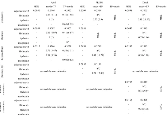
4.2. Summary results for 1-hour models
The overall estimation results for the 1-hour models are summarised in Table 6, giving the estimates for the three nesting parameters along with the adjusted 2measure. Whenever the estimate for a nesting parameter took on an unacceptable value, it was constrained to a value of 1 in re-estimation, and this is indicated in the table through the absence of a t-ratio for that parameter. Again, the asymptotic t-ratios for the nesting parameters were calculated with respect to a value of 1.
The results show that, for the APRIL data, the NL model with TP choice above mode choice is the preferred structure for commuters, while the NL model with mode choice above TP choice is the preferred structure for leisure travel. For business travellers, the two NL models are equivalent, as only SPchscale
takes on an acceptable value. Both models outperform the MNL model, by recognising the correlation between SP car alternatives associated with the same time period.
7 These values were collected across 7 different models, of which only four are shown in Table 3, where the others were lacking some of
For the PRISM data, the model nesting TP choice above mode choice is rejected in all purpose segments, with the nesting parameters taking on unacceptable values. For commuters, the model nesting mode choice above TP choice outperforms the MNL model, with the same being the case in the models for leisure travellers and the model for home-based business tours. In the combined models for all business travellers (home-based and non-home-based), both NL models lead to unacceptable values for the structural parameters, while it was not possible to estimate a separate model for non-home-based business trips, with the models failing to converge, independently of model structure.
For the Dutch data, the model nesting TP choice above mode choice is rejected in all purpose segments, due to unacceptable values for the nesting parameters. Other than that, the model nesting mode choice above TP choice is the recommended structure for commuters and leisure travellers, while the difference to the MNL model is very small in the case of business travellers. Finally, the same structural conclusions arise when using separate models for flexible and inflexible commuters.
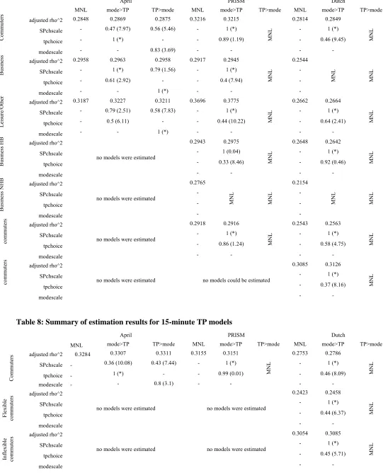
4.3. Summary results for coarse models
The overall results for the models using the coarse TP formulation are summarised in Table 7. For the APRIL data, we again observe that, for commuters, the model nesting TP choice above mode choice is the preferred structure. In the two remaining segments (business and leisure), the model nesting mode choice above TP choice is the preferred structure. These results are thus consistent with the findings for the one-hour models.
For the PRISM data, the model nesting TP choice above mode choice is again rejected in all purpose segments, as the nesting parameters take on unacceptable values. The model nesting mode choice above TP choice rejects the MNL model in the leisure segment. The same is the case for the common model for all business travellers, while, in the submodels for home-based and non-home-based business travellers, this is only the case for the former, while, for the latter, MNL is the preferred structure. Finally, for commuters, the NL model nesting mode choice above TP choice fails to outperform the MNL model, where in addition, it was not possible to estimate a submodel for inflexible commuters, due to a failure to converge.
For the Dutch data, the model nesting TP choice above mode choice is again rejected in all purpose segments. While the model nesting mode choice above TP choice fails to reject the MNL model in the case of commuters and leisure travellers, it is the preferred structure for business travellers.
4.4. Summary results for 15-minute models
Models using the 15-minute TP specification were only estimated for commuters, where, in the Dutch data, separate models were also estimated for flexible and inflexible commuters. Consistent with the findings for the one-hour and coarse models, the model nesting TP choice above mode choice is again the preferred structure in the APRIL data (cf. Table 8). In the PRISM data, the MNL model cannot be rejected by the data, as discussed in Section 4.1. Finally, with the Dutch data, the model nesting mode choice above TP choice is the preferred structure, independently of whether a joint model is used for all commuters or whether separate models are estimated for flexible and inflexible commuters.
4.5. Overall results
leads to a loss of significance of the nesting of time period below mode. The findings from the APRIL data differ from those on the other two data sets, and is useful to note that the models based on that data are generally of rather lower quality, while the presentations to travellers were somewhat different. The weight attached to these results should perhaps be considered to be less than the weights attached to the results from the other two data sets.
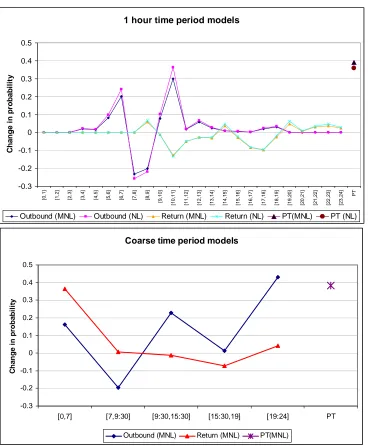
5. FORECASTING EXAMPLE
As a final extension of the research, a brief forecasting application was conducted, showing the predicted changes in choice probabilities following the introduction of a notional charge of £2 during the 7AM-9AM peak period. For this, we used the data on commuters in the West Midlands. The results are summarised in Figure 5, showing the changes in the average probabilities in the different time periods for car travel and for the public transport alternatives (aggregated across time periods). Given the different context for the 15-minute models (outbound travel only), this forecasting example makes use only of the 1-hour and coarse time period models.
Looking first at the 1-hour models, we can clearly see a shift away from the eight and ninth time period for the outbound journey, i.e. the two periods with congestion charging. Substitution is greater to the shoulder of the peak period than to the off-peak period, consistent with intuition. Although the difference between the MNL and NL results is rather small, the NL results do show a smaller shift towards public transport than the MNL results, along with a greater shift towards other time periods. Finally, we look at the elasticity for public transport relative to the cost of car travel. For the recommended model, NL with mode nested above TP, we obtain a change in probability for public transport by 35.9% following an increase in the cost of car travel by £2. With an average cost of £2.70 for car travel in the data, we thus get an elasticity of 35.9/74.1=0.48. This is higher in the MNL model, where the elasticity is 0.53.
With the coarse time period specification, we also obtain a higher elasticity for public transport, at 0.52. Finally, we see a shift in probability to the two time periods adjacent the charged period, but there is also an increase for evening travel. This latter period however had very low initial probability (<1%), so this needs to be put into context.
Before closing, it should be acknowledged that the elasticities are higher than might have been expected. The lowest (and most realistic) value is obtained from the NL model nesting mode choice above time period choice with the 1-hour specification, while a MNL specification leads to higher elasticities with both time period specifications reported here. As a check on the reasonableness of these forecasting results, comparisons may be made with the mode switching results of the PRISM model (RAND Europe, 2005b). PRISM is based primarily on RP data and gives an elasticity for public transport demand with respect to car cost substantially lower (around 0.10) than indicated in the model estimated in this work using exclusively SP data. However, when we consider the potential impacts of the selection of the SP data, the fact that PRISM also considers destination switching and several modes other than car driver and public transport, and the fact that it may generally be expected that SP responses are more elastic than RP responses, then such a difference is to be expected. Additionally, the forecasting results of de Jong et al. (2003), who apply MMNL models to the Dutch SP data analysed in this paper, seem to be consistent with the NL results shown here.
6. SUMMARY AND CONCLUSIONS
in this paper, on the basis of an extensive analysis making use of three separate SP datasets collected in the United Kingdom and the Netherlands.
The analysis showed that, in the models estimated for the PRISM data and the Dutch data, the best model performance (in terms of adjusted 2 measure) was obtained with the one-hour specification for the time periods, ahead of the coarse specification and the specification using 15-minute intervals. For the APRIL data, the performance is very similar across specifications, with the exception being a notable gain in performance with the 15-minute models for commuters. Overall however, the differences are rather small, and comparisons are difficult, given the use of slightly different sample sizes (as well as segmentations) across specifications. In practical studies, other considerations would outweigh these issues of model quality. In terms of correlation structure, the analysis shows that, with a few exceptions, the nested models outperform the basic MNL structures, which operate under the assumption of equal substitution patterns across alternatives. The advantages of the nesting structures are especially pronounced in the one-hour and 15-minute models, but, in the coarse models, the broader specification of the time periods clearly results in lower substitution between time periods, as a similarly sized shift in departure time is now less likely to lead to a jump to a different time period. However, some interesting differences arise. In the PRISM and Dutch data, the models nesting TP choice above mode choice are unacceptable, independent of the purpose segment or the specification used for the time periods. On the other hand, for the APRIL data, the models nesting TP choice above mode choice not only always outperform the MNL model, but in fact also reject the model nesting mode choice above TP choice in the case of commuters.
As such, the results of this analysis suggest that, with the exception of commuters in the APRIL data, there is higher substitution between alternative time periods than between alternative modes (always under ceteris paribus), showing that, for the three specification of time period lengths studied, travellers are more sensitive to transport levels of service in their choice of departure time than in their choice of mode. The results reported here also indicate that the sensitivity is greater for switches between shorter than between longer time periods. A model for switching to shoulders of the peak (i.e. a smaller shift in departure time) would therefore have greater sensitivity than a model for switching between peak and off-peak periods. These findings are again consistent between the earlier models using continuous departure time information and the models estimated with time period data.
The summary finding of the work is that the sensitivity of time period choice to travel times and costs is generally greater than that of mode choice. This is consistent with the findings reported by Hess et al. (2006) for the parallel analysis making use of continuous departure time information (see Section 3.1). However, in closing, it should again be noted that the opposite was observed in the case of commuters in the APRIL dataset. As such, it would be desirable that the results should be confirmed by further study in other areas.
ACKNOWLEDGEMENTS
The work reported in this paper was supported by the UK Department for Transport. The opinions presented in this paper are those of the authors and do not necessarily represent the views of the Department. The authors would like to thank the West Midlands local authorities and the Netherlands Ministry of Transport for their cooperation in granting permission to use their data. We are grateful for the constructive comments of two anonymous referees on an earlier version of this paper, who have helped us to clarify our work. We retain responsibility for any remaining errors or misinterpretations.
REFERENCES
Bates, J.J. and I.N. Williams (1993) APRIL – A strategic model for road pricing, Proceedings of Seminar D, PTRC Summer Annual Meeting, 1993. PTRC Education and Research Services Ltd, London.
Daly, A. J. (1987) Estimating ‘Tree’ Logit Models, Transportation Research, 21B, pp 251- 267.
De Jong, G., Daly, A., Pieters, M., Vellay, C. and Hofman, F. (2003) A model for time of day and mode choice using error components logit, presented to European Transport Conference, Cambridge (2001), revised version published in Transportation Research (E) 29, pp. 246–268.
Domencich, T.A. and McFadden, D. (1975) Urban Travel Demand : A behavioural analysis, North Holland, Amsterdam.
Hess, S., Polak, J.W. and Bierlaire (2005). Functional approximations to alternative specific constants in time period choice-modelling, proceedings of the 16th International Symposium on Transportation and Traffic Theory, University of Maryland, College Park, MD.
Hess, S., Polak, J., Daly, A. and Hyman, G., (2006) Flexible substitution patterns in models of mode and time-of-day choice: new evidence from the UK and The Netherlands, Transportation, forthcoming.
McFadden, D. (1978), Modelling the choice of residential location, in A. Karlquist, ed., ‘Spatial Interaction Theory and Planning Models’, North Holland, Amsterdam, chapter 25, pp. 75–96.
McFadden, D. (1981) Econometric models of probabilistic choice. In Manski, C. and McFadden, D. (eds) Structural Analysis of Discrete Data: With Econometric Applications. The MIT Press, Cambridge, Massachusetts.
McFadden, D. & Train, K. (2000), ‘Mixed MNL Models for discrete response’, Journal of Applied Econometrics 15, 447–470.
Polak, J.W. and P.M. Jones (1994) A tour-based model of journey scheduling under road pricing, Paper presented at the 73rd Annual Meeting of the Transportation Research Board, Washington, D.C.
RAND Europe (2004), PRISM West Midlands: Time of Day Choice Models, RED-02061-04, available from
http://www.prism-wm.com.
RAND Europe (2005a), Departure Time and Mode Choice: an analysis of three stated preference data sets, available from
www.dft.gov.uk/stellent/groups/dft_econappr/documents/divisionhomepage/040158.hcsp
RAND Europe (2005b), PRISM West Midlands: Tour Based Mode Destination Modelling, RED-02061-05, available from http://www.prism-wm.com.
Small, K. (1987), ‘A discrete choice model for ordered alternatives’, Econometrica 55(2), 409–424. Train, K. (2003). Discrete Choice Methods with Simulation, Cambridge University Press, Cambridge, MA. Williams, H. C. W. L. (1977), ‘On the Formulation of Travel Demand Models and Economic Evaluation
Measures of User Benefit’, Environment & Planning A 9(3), 285–344.
Table 1: Required departure time shift in minutes for sensitivity to time-shifting to be equal to
sensitivity to mode-shifting (from Hess et al., 2006)
PRISM data Dutch data
EC early-shift EC late-shift EC early-shift EC late-shift
Commuters flexible 189 205 333 N/A
Commuters non-flexible 108 47 355 226
Business travellers 1037 286
Other 307 316 175
Table 2: Specification of time periods in coarse models
Period PRISM data Dutch data APRIL data
Table 3: Estimation results for 1-hour TP models for commuters in PRISM data
Model: MNL NL mode>TP NL mode>TP NL TP>mode
Observations: 2922 2922 2922 2922
LL(0): -3680.66 -3680.66 -3680.66 -3680.66
Final LL: -2413.8 -2382 -2410.8 -2384.5
Parameters: 49 51 50 51
adjusted 2(0): 0.3309 0.3390 0.3314 0.3383
est. asy.t-rat. est. asy.t-rat. est. asy.t-rat. est. asy.t-rat.
PT -2.59 -16.2 -2.82 -12.9 -2.88 -13.1 -2.58 -14.6
TTC -0.0245 * -0.0245 * -0.0245 * -0.0245 *
TTPT -0.0314 * -0.0314 * -0.0314 * -0.0314 *
TC -0.0086 * -0.0086 * -0.0086 * -0.0086 *
early (flexible) -2.8 -13.7 -2.68 -11.7 -2.48 -12.4 -3.01 -12.7
early (inflexible) -3.89 -15.1 -3.85 -12 -3.39 -12.7 -4.38 -13.8
late (flexible) -2.99 -14.1 -2.74 -11.8 -2.64 -12.5 -3.06 -12.7
late (inflexible) -5.32 -15.1 -4.84 -11.9 -4.61 -12.5 -5.51 -13.7
duration(0) -0.388 -0.3 -0.455 -0.4 -0.292 -0.3 -0.541 -0.4
duration(1) 0.279 0.3 -0.0191 0 0.304 0.3 -0.0826 -0.1
duration(2) -0.247 -0.3 -0.459 -0.6 -0.146 -0.2 -0.582 -0.6
duration(3) 0.139 0.2 -0.0075 0 0.188 0.3 -0.0775 -0.1
duration(4) -0.0036 0 -0.0443 -0.1 0.0554 0.1 -0.113 -0.2
duration(5) 0.105 0.2 0.119 0.3 0.104 0.2 0.118 0.2
duration(6) -0.0527 -0.2 -0.0686 -0.2 -0.0534 -0.2 -0.0685 -0.2
duration(7) -0.641 -2.8 -0.597 -2.7 -0.572 -2.8 -0.659 -2.7
duration(8) 0 * 0 * 0 * 0 *
duration(9) 0.0175 0.1 0.0601 0.3 0.001 0 0.0761 0.4
duration(10) -0.179 -0.5 -0.141 -0.4 -0.162 -0.5 -0.153 -0.4
duration(11) -0.192 -0.4 -0.156 -0.3 -0.241 -0.5 -0.0987 -0.2
duration(12) 0.366 0.5 0.247 0.3 0.189 0.3 0.406 0.5
duration(13) -0.854 -0.8 -0.835 -0.9 -0.835 -0.9 -0.862 -0.8
ret(9) -1.83 -1.2 -1.38 -1 -1.76 -1.3 -1.39 -0.9
ret(10) -1.31 -1.1 -0.868 -0.8 -1.29 -1.2 -0.835 -0.7
ret(11) -4.1 -3.7 -3.29 -3.2 -3.64 -3.7 -3.66 -3.2
ret(12) -2.03 -2.3 -1.55 -1.9 -1.88 -2.4 -1.65 -1.8
ret(13) -1.69 -2.2 -1.33 -1.9 -1.61 -2.4 -1.38 -1.7
ret(14) -0.35 -0.5 -0.183 -0.3 -0.472 -0.8 -0.0287 0
ret(15) -0.428 -0.9 -0.318 -0.7 -0.508 -1.2 -0.218 -0.4
ret(16) -0.293 -0.8 -0.299 -0.9 -0.364 -1.2 -0.225 -0.6
ret(17) 0.114 0.5 0.0835 0.4 0.07 0.3 0.118 0.5
ret(18) 0 * 0 * 0 * 0 *
ret(19) -0.589 -2 -0.628 -2.3 -0.624 -2.3 -0.589 -1.9
ret(20) -1.86 -3.6 -1.7 -3.7 -1.71 -3.8 -1.84 -3.5
ret(21) -3.05 -3.4 -2.61 -3.3 -2.82 -3.6 -2.77 -3
ret(22) -0.243 -0.3 -0.203 -0.3 -0.36 -0.5 -0.0509 -0.1
ret(23) -1.25 -1 -0.901 -0.8 -1.13 -1 -0.97 -0.7
ret(24) -3.83 -2.7 -3.74 -2.9 -3.48 -2.8 -4.08 -2.8
out(4) -2.43 -1.5 -1.59 -1.2 -2.08 -1.5 -1.82 -1.1
out(5) -3.15 -3.6 -2.7 -3.3 -2.74 -3.6 -3.07 -3.3
out(6) -1.12 -3.1 -0.822 -2.5 -1.01 -3.2 -0.877 -2.3
out(8) 0 * 0 * 0 * 0 *
out(9) 0.237 1.3 0.191 1.1 0.224 1.4 0.192 1
out(10) -0.308 -1.1 -0.223 -0.8 -0.304 -1.2 -0.226 -0.7
out(11) -0.741 -1.7 -0.506 -1.3 -0.733 -1.9 -0.486 -1.1
out(12) -2.51 -2.7 -2.13 -2.6 -2.16 -2.7 -2.49 -2.6
out(13) -4.08 -4 -4.07 -4.4 -3.61 -4.1 -4.61 -4.4
out(14) -1.94 -1.4 -2.13 -1.7 -1.77 -1.5 -2.38 -1.7
out(15) -0.407 -0.2 -0.574 -0.4 -0.489 -0.3 -0.543 -0.3
out(16) 2.55 1.7 2.17 1.6 2.12 1.6 2.54 1.7
out(17) 1.97 1.3 1.56 1.1 1.61 1.2 1.86 1.2
out(18) -1.36 -0.8 -1.51 -1 -1.29 -0.9 -1.64 -1
out(19) 0.276 0.1 0.121 0.1 0.142 0.1 0.213 0.1
SPscale 0.574 14.18 0.383 14.18 0.677 6.25 0.328 20.49
tpchoice 1 * 0.769 2.82 0.77 2.89
SPchscale 1 * 1.78 5.52 1 * 1.68 3.48
modescale 1.06 0.66
Notes to Tables 3-9
Coefficients with t-ratios indicated by ‘*’ are fixed.
Table 4: Estimation results for coarse TP models for commuters in the PRISM data
Model: MNL NL mode>TP NL TP>mode
Observations: 2929 2929 2929
LL(0): -3702.85 -3702.85 -3702.85
Final LL: -2492 -2491.4 -2487.3
Parameters: 20 21 22
adjusted 2(0): 0.3216 0.3215 0.3223
PT -2.6 -16 -2.75 -12.6 -2.58 -14.8
TTC -0.0245 * -0.0245 * -0.0245 *
TTPT -0.0314 * -0.0314 * -0.0314 *
TC -0.0086 * -0.0086 * -0.0086 *
early (flexible) -2.94 -15.3 -2.78 -12.7 -3.03 -12.6
early (inflexible) -4.02 -16.4 -3.77 -12.5 -4.17 -12.7
late (flexible) -3.12 -15.5 -2.95 -12.8 -3.18 -12.5
late (inflexible) -5.44 -16 -5.1 -12.2 -5.59 -12.3
out(1),return(1) 0.88 0.4 0.723 0.3 1.11 0.5
out(1),return(2) 0.594 0.9 0.506 0.8 0.846 1.2
out(1),return(3) -0.955 -3.4 -0.94 -3.6 -0.707 -2.4
out(1),return(4) -0.333 -1.6 -0.343 -1.8 -0.162 -0.8
out(1),return(5) -1.66 -2 -1.54 -2 -1.34 -1.6
out(2),return(2) 1.45 1.8 1.32 1.7 1.5 1.8
out(2),return(3) -0.0079 0 -0.0193 -0.1 0.102 0.4
out(2),return(4) 0 * 0 * 0 *
out(2),return(5) -2.99 -4 -2.84 -4.1 -2.74 -3.7
out(3),return(3) 0.264 0.7 0.231 0.6 0.527 1.3
out(3),return(4) -0.847 -3.2 -0.816 -3.3 -0.61 -2.3
out(3),return(5) -1.7 -4.1 -1.66 -4.2 -1.48 -3.5
out(4),return(4) 2.33 2.1 2.13 2 2.25 2
out(4),return(5) -2.07 -2.8 -1.98 -2.9 -2.1 -2.9
out(5),return(5) -3.76 -1.5 -3.54 -1.5 -3.83 -1.6
SPscale 0.552 15.50 0.596 8.27 0.501 11.35
tpchoice 1 * 0.887 1.19
SPchscale 1 * 1 * 1.09 0.82