Prediction Intervals for Reliability Growth Models with Small Sample Sizes Summary
The first section within this chapter provides an introduction into the types of test being considered for this growth model and a description of the two main forms of uncertainty encountered within statistical modelling, namely aleatory and epistemic. These two forms are combined to generate prediction intervals for use in reliability growth analysis. The second section of this chapter provides an historical account of the modelling form used to support the prediction intervals. An industry standard model is described and will be extended to account for both forms of uncertainty in supporting predictions about the time to the detection of the next fault
The third section of this chapter describes the derivation of the prediction intervals. The approach to modelling growth uses a hybrid of Bayesian and Frequentist approaches to statistical inference. A prior distribution is used to describe the number of potential faults believed to exist within a system design, while reliability growth test data is used to estimate the rate at which these faults are detected.
After deriving the prediction intervals, the fourth section of this chapter provides an analysis of the statistical properties of the underlying distribution for a range of small sample sizes.
The fifth section gives an illustrative example used to demonstrate the computation and interpretation of the prediction intervals within a typical product development process.
1 Introduction
Predicting the time until a fault will be detected on reliability growth test is complex due to the interaction of two sources of uncertainty and hence often results in wide prediction intervals that are not practically credible. The first source of variation corresponds to the selection of an appropriate stochastic model to explain the random nature of the fault detection process. The second source of uncertainty is associated with the model itself, as even if the underlying stochastic process is known, the realisations will be random. Statistically, the first source of uncertainty can be measured through confidence intervals. However to use these confidence intervals for prediction can result in naïve under-estimates of the time to realise the next failure because they will only provide inference on the mean time to the next fault detection rather than the actual time of the fault detection. Since the confidence in parameter estimates increase as sample size increase, the degree of underestimation arising from the use of confidence rather than prediction intervals will be less for large sample sizes compared with small sample sizes. Yet, in reliability growth tests it is common, indeed desirable, to have a small number of failures. Therefore there is a need for prediction intervals, although their construction is more challenging for small samples since they are driven by the second source of variation.
This cyclical process is repeated until all weaknesses have been flushed out and the system design is deemed mature. The data generated through test are analysed using reliability growth models and the information generated is used to support product development decisions. For example, the duration of the growth test to achieve required reliability or the efficacy of the stresses experienced by the prototype designs during test within a specified test plan.
Procedures for the construction of prediction intervals for the time to realise the next failure are developed for a standard reliability growth model called the Modified IBM model. This model is particularly suited for test situations where few data exist and some expert engineering judgment is available. The model consists of two parameters: one that reflects the number of faults within the system design; and a second that reflects the rate at which the faults are detected on test. Estimation procedures have been developed as a mixture of Bayesian and Frequentist methods. Processes exist to elicit prior distributions describing the number of potential faults within a design. However prior distributions describing the test time by which these faults will be realised are more challenging to elicit and as such inference for this parameter is supported with the data observed from the test.
to a typical reliability growth test. Finally the use of such procedures is reflected upon in section 6.
2 Modified IBM Model – A Brief History
The IBM model was proposed by [1] and was the first reliability growth model to formally represent two different types of failures: namely those that result in a corrective action to the system; and those that result in a replacement of a component part. By formally accounting for failures that occur but which are not addressed at the system level, the failure rate is estimated by an asymptote corresponding to a residual failure rate relating to faults that would have been detected and corrected, but were not due, to the termination of testing. The model was developed assuming the following differential equation:
( )
( ), , 0
µ µ
= − >
d D t
D t t
d t (1)
whereD t
( )
represents the number of faults remaining in the system at accumulated test time t. Therefore the expected number of faults detected by accumulated test time t is:( )
(
)
( ) 0 1 t , , 0
The model proposes that spurious failures would be realised according to a Homogeneous Poisson Process independent of the fault detection process. This latter process is not of direct concern to the model developed here and hence we do not develop further. Instead we focus on the fault detection process only.
The deterministic approach to reliability growth modelling was popular in the late 1950’s and early 1960’s. However this approach was superseded by the further development and popularity of statistical methods based upon stochastic processes. This is because the deterministic arguments regarding the reliability growth could just as easily be interpreted through probabilistic methods, which also facilitated more descriptive measures for use in test programmes.
Cozzolino [2] arrived at the same form for an intensity function, ι
( )
t , assuming that the number of initial defects within a system, D( )
0 , has a Poisson distribution with mean λ and the time to failure of each initial defect followed an exponential distribution with hazard rate µ.:( )
t , e- µt , ,t 0ι =λµ µ λ > (3)
( )
1- e(
- t)
E N t =λ µ (4)
Jelenski and Moranda [3] proposed a model to describe the detection of faults within software testing assuming that there were a finite number of faults (i.e. D
( )
0 ) within the system and that the time between the detection of the ith and(
i−1)
th ( i.e.i
W) fault had the following exponential Cumulative Distribution Function (CDF):
( )
( )
( 0 1)
( ) 1 D i wi, 1, 2,..., 0 ; , 0
i i
F w = −e− − + µ i= D w µ > (5)
This model is the most referenced software reliability model [4]. It is assumed for this model that there exists D
( )
0 faults within system whose times of failure are all independently and identically exponentially distributed with hazard rate µ.. It is interesting to note the similarities between this model, Cozzolino’s model (4) and the IBM (2) deterministic model, as in this model the mean number of faults detected at time accumulated test time t is the same in all three models.Meinhold and Singpurwalla [7] proposed an adaptation with a Poisson prior distribution to estimate the number of faults that will ultimately be exposed. This is similar to Cozzolino [2] but from a Bayesian perspective, so the variability described through the prior distribution captures knowledge uncertainty in the number of faults within the system design only. This Bayesian approach results in the following estimating equation for µ: ' 2 1 1 ' ... , ˆ ' t t t t t e t j j j i i t ≤ < < < + =
∑
= − µ λµ (6)
Where: ti is the time of the ith fault detected on test t' is the test time when the analysis is conducted
j is the number of faults detected by time t'
This Bayesian adaptation was further explored in [8] and it’s advantages over the industry standard model, the so-called Power Law model [9, 10] was demonstrated. A process was developed to elicit the prior distribution for this model in [11] and procedures for estimating confidence intervals for µ were developed in [12]. Extensions of this model to assess cost effectiveness of reliability growth testing are addressed in [13] and for managing design processes see [14]. This model is incorporated into the international standard, IEC 61164, as the Modified IBM model.
times to detect faults that are independently and identically exponentially distributed. A prior distribution describing the number of faults existing within the system design is assumed to be a Poisson. Finally, it is assumed that when a fault is identified it is removed completely and no new fault is introduced into the design.
3 Derivation of Prediction Intervals for Time to Detection of Next Fault
We assume that a system contains D
( )
0 faults. The time to detect a fault is exponentially distributed with hazard rate µ. and a prior distribution exists on D( )
0 , in the form of a Poisson distribution with mean λ. It is further assumed that j faults will be observed on test at times t1,....tj and we seek a prediction interval for the time to detect the next fault, i.e. x, where it is assumed the times to detection are statistically independent.The statistic R is defined as the ratio of x to the sum of the first j fault detection times, denoted by T:
x R
T
= (7)
with hazard rate µ. Thus, the time between any two consecutive such Order Statistics are exponentially distributed with hazard rate
(
D( )
0 − +i 1)
µ. Moreover, the times between successive Order Statistics are independent. For a derivation of this results see [15]. Therefore T can be expressed as a weighted sum of independent and identically distributed exponential random variables with hazard rate µ. We denote these random variables as Wi in the following:1 1 1 1 j i i j i i T t j i W N i = = = − + = − +
∑
∑
(8)As an exponential random variable is closed under scale transformation, we can consider
T, as expressed in (8), as a sum of independent exponential random variables with different hazard rates. As such, using Goods formula [16] we can express the CDF of T, conditioned on there being j faults realised and the design initially having D
( )
0 faults, as:(
)
( )
- 1-- 1
1 1 1
- 1
- 1 - 1
Pr , 0
1-- 1 - 1
- 1
- 1 - 1
n i j
j j t
i j i
i i k
k i
n k
j i W j k
t j D n e
n k n i
n i
j k j i
µ + + = = = ≠ +
+ < = = +
+ + + − + +
∑
∑∏
(9)( )
(
)
( )
( )
(
)
(
)
0
0 , 0 ,
0 , ,
x
P R r D j P r D j
T
P x rt D j T t P T t dt
∞
< = <
=
∫
< = =(10)
Since we know that x will have an exponential distribution with hazard rate
( )
(
D 0 − j)
µ, we obtain:( )
(
)
( )(
)
(
)(
)
(
)
- 1 -- 1 1 1 0 1 1 - 1 - 1 - 1 0 1- 1 - 1 - 1
- 1 - 1
- 1
- 1 - 1
1
- 1 - 1
- 1 - 1
- 1 - 1
n i j
j t
n j rt j i
i k t k i j j i k k i n k n i j k
P R r D n e e dt
n k n i j i
j k j i
n k
n i j k
n k n i
n i j i n j r
j k j i
µ µ µ + ∞ − − + = = = ≠ = = ≠ + + +
< = = − + +
+ − + + + + + = − + + + + + − − + +
∑∏
∫
∑
∏
(11)This probability distribution is a pivotal since it does not depend on µ and can therefore be used to construct a prediction distribution for the time to detect the next fault. (11) can be simplified to give:
( )
(
)
(
) (
)
(
) ( )
(
)(
)
(
)
(
) (
)
1 1 1 1- 1 1
!
0 1
- 1 - 1 1 ! !
! j i j j i j i n
P R r D n
n i j i n j r i j i
n j n j
− −
− =
+ −
< = = −
+ + + − − −
− −
∑
Taking the expectation with respect to D
( )
0 , for which it is assumed we have a Poisson prior distribution, provides a CDF that can be used to obtain prediction intervals. The CDF in (13) for the ratio, i.e. R, is calculated assuming there is at least one more fault remaining in the system design. The probability that all faults have been exposed given there has been j faults detected is expressed in (14):
( )
(
)
(
) (
)
(
) ( )
(
)(
)
(
)
(
) (
)
1 1 1 1 1 0- 1 1
!
!
- 1 - 1 1 ! !
!
0 1, 1
1
!
j i n
j
j
n j i
k j k j i n e n
n i j i n j r i j i
n j n j
P R r D j j
e k λ λ λ λ − − − ∞ − = + = − = + − + + + − − − − −
< ≥ + = −
−
∑
∑
∑
(13)
(
)
10 ! 1 ! j k j k e j
P R j
e k λ λ λ λ − − − = = ∞ = −
∑
(14)Consider how this distribution changes as we expose all faults within the design. As the number of faults detected, j, increases towards D
( )
0 , then the distribution of Tapproaches a gamma distribution as follows:
( ) ( )
( )
( )
0 0 1
0 1 1 lim lim 1 lim 0 1 j i
j D j D i
j
i
j D i
where Wi are independent and identically exponentially distributed and their sum has a gamma distribution with parameters j and µ. Therefore, as j approaches D
( )
0 , the distribution of R should approach the following:( )
(
)
(
( )
)
(
)
0
0 , 0 , ,
1 1
1
j
P R r D n j P x rt D n j T t P T t dt
r
∞
< = = < = = =
= − +
∫
(15)
Computationally, (15) will be easier to apply than (13), assuming there exists at least one more fault in the design. In the following section the quality of (15) as an approximation to (13) will be evaluated.
4 Evaluation of Prediction Intervals for Time to Detect Next Fault
The model assumes the time between the ith and (i+1)th fault detection is exponentially
distributed with hazard rate µ
(
D( )
0 −i+1)
. Consequently, if D( )
0 increases then the expected time to realise the next fault reduces. Therefore as λ, which is the expectation of D( )
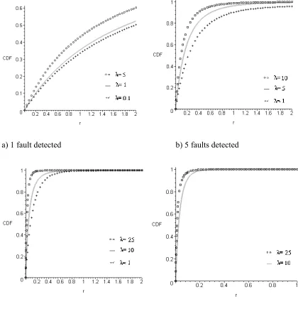
0 increases, the CDF for the ratioRshifts upwards. This is illustrated in Figure 1, where the CDF in (13) is shown for various values of λ assuming there have been 1, 5, 10 and 25 faults detected.a) 1 fault detected b) 5 faults detected
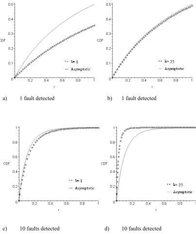
[image:14.595.85.505.164.599.2]a) 1 fault detected b) 1 fault detected
[image:15.595.82.486.152.634.2]The data in the plots in Figures 1 and 2 has been generated using Maple version 8 that has been used to support numerical computations. To avoid the need to reproduce calculations, summaries of key characteristics of the CDF are presented in the following tables.
Table 1 Values of the mean of the distribution of R
j\λ 1 5 10 15 20
1 ∞ ∞ ∞ ∞ ∞
2 1.60 1.13 0.86 0.78 0.76 3 0.74 0.52 0.36 0.31 0.3 4 0.46 0.34 0.22 0.18 0.17 5 0.33 0.25 0.16 0.12 0.11 10 0.13 0.11 0.08 0.05 0.04
Table 2 Values of the median of the distribution of R
J\λ 1 5 10 15 20 1 1.82 1.32 1.13 1.08 1.06 2 0.65 0.45 0.35 0.32 0.31 3 0.37 0.26 0.18 0.16 0.15 4 0.26 0.18 0.12 0.10 0.09 5 0.20 0.14 0.09 0.07 0.06 10 0.09 0.07 0.05 0.03 0.02
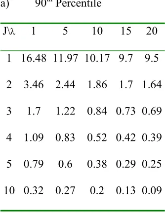
[image:18.595.87.254.516.732.2]Table 3 presents summaries of the 90th, 95th and 99th percentiles of the distribution of R. The skew is noticeable by the difference between the 95th and 99th percentile, where there is a larger difference for the situation where there have been fewer faults detected.
Table 3 Percentiles of the distribution of R
a) 90th Percentile
J\λ 1 5 10 15 20
b) 95th Percentile
j\λ 1 5 10 15 20
1 34.83 25.31 21.49 20.48 20.06 2 5.58 3.96 3 2.73 2.64 3 2.54 1.85 1.27 1.09 1.03 4 1.57 1.18 0.77 0.61 0.56 5 1.11 0.87 0.56 0.41 0.36 10 0.43 0.37 0.28 0.18 0.12
c) 99th Percentile
j\λ 1 5 10 15 20
5 Illustrative Example
This example is based around the context and data from a reliability growth test of a complex electronic system. A de-sensitised version of the data is presented, however this does not detract from the key issues arising through this reliability growth test and the way in which the data are treated. The aim of this example is to illustrate the process of implementing the Modified IBM (MIBM) model for prediction and to reflect upon the strengths and weaknesses of this approach
5.1 Construction of Predictions
A TAAF test regime has been used in this growth development test. The duration of the test was not determined a priori but was to be decided based upon the analysis of the test data. Two units have been used for testing. Both units have been tested simultaneously. The test conditions were such that they approximated the stress levels expected to be experienced during operation.
realised as a fault during test. Group interviews are conducted were overlapping concerns are identified to explore correlation in the assessment. The probabilities are convoluted to obtain a prior distribution describing the number of faults that exist within the design. Typically a Poisson distribution provides a suitable form for this prior and as is assumed within the MIBM model. For this illustration we use a Poisson distribution with a mean of 15.
The test was conducted for a total of 7713 test hours. This was obtained by combining the exposure on both test units. Nine faults were exposed during this period. Figure 3 illustrates the cumulative number of faults detected against test time. Visually, there is evidence of reliability growth, as the curve appears concave, implying the time between fault detection is, on average, decreasing. There was two occasions where faults were detected in relatively short succession: this occurred between 3000 to 4000 hours and 6000 to 7000 hours.
Figure 3 Faults detected against accumulated test time
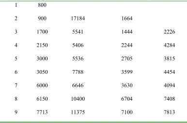
Table 4 provides a summary of the estimates provided by the MIBM and these are also illustrated in Figure 4. The median estimator appears to perform better than the mean. This is due to the large skew in the tail of the distribution of the predicted ratio resulting in a mean much greater than the median. All nine faults were observed at earlier times than the upper 95% prediction limit. The point estimates were poorest at the time of the seventh fault detection, which had been realised after an unusually long period of no fault detection.
0 1 2 3 4 5 6 7 8 9
0 1000 2000 3000 4000 5000 6000 7000 8000 9000 Accumulated Test Time
Figure 4 Comparison between actual and model prediction fault detection times
Table 4 Predictions of fault detection times based on model
Fault Number Actual Upper 95% Prediction Median Prediction Mean Prediction 1 800
2 900 17184 1664
3 1700 5541 1444 2226
4 2150 5406 2244 4284
5 3000 5536 2705 3815
6 3050 7788 3599 4454
7 6000 6646 3630 4094
8 6150 10400 6704 7408
0 1000 2000 3000 4000 5000 6000 7000 8000 9000
0 1 2 3 4 5 6 7 8 9
Fault Detected
Ac
cu
mul
ated Test T
ime
[image:23.595.89.475.482.735.2]Table 5 provides the point estimate of the number of faults remaining undetected within the design at each fault detection time. This is obtained using the formula (16), the derivation of which can be found in [12]. The MLE of µ was substituted in place of the parameter:
( )
0( )
tE D −N t µ=λe−µ
[image:24.595.90.462.424.674.2] (16)
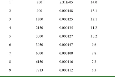
Table 5 Expected faults remaining undetected
Fault detected Accumulated Test Time ^
µ Expected Faults Remaining
1 800 8.31E-05 14.0
2 900 0.000148 13.1
3 1700 0.000125 12.1
4 2150 0.000135 11.2
5 3000 0.000127 10.2
6 3050 0.000147 9.6
7 6000 0.000108 7.8
8 6150 0.000116 7.3
Table 5 provides some reassurance of the model we are using for this process. The expected number of faults remaining undetected decreases in line with the detection of the faults and there is some stability on the estimation of µ.
The analysis conducted to obtain predictions assumes that there is at least one more fault remaining undetected within the design. However, we are assuming that there are a finite number of faults within the design described through the Poisson prior distribution with a mean of 15 at the start of test. Table 6 provides the probability that all faults have been detected at each fault detection times. This is a conditional probability calculated from the Poisson distribution. The formula used assuming j faults have been detected and a mean of λ provided in (17):
( )
( )
(
)
10 !
0 '
1
!
j
k j
k
e j
P D j N t j
e k
λ
λ
λ
λ
−
− −
=
= = =
−
∑
(17)
Table 6 Probability of having detected all faults Number of faults
detected
Probability all faults have been detected
1 4.58854E-06 2 3.44142E-05 3 0.0002 4 0.0006 5 0.0019 6 0.0049 7 0.0105 8 0.0198 9 0.0337
5.2 Diagnostic Analysis
Although visually the model appears to describe the variability within the data, the formal assessment of the validity of the CDF of the ratio is assessed in this section.
detections and the sum of the proceeding fault detection times. Our hypothesis is that these observations have been generated from the CDF. Table 7 presents a summary of the observed ratio and the percentile to which the ratio corresponds in the CDF. Assuming the model is appropriate then these observed percentiles should be consistent with eight observations being observed from a uniform distribution over than range [0,1]. These percentiles appear to be uniformly distributed across [0,1] with possibly a slight central tendency between 0.6 and 0.7, however this is not necessarily statistically significant.
Table 7 Observed Ratios
A formal test can be constructed to assess whether the percentiles in Table 7 are appropriately described as belonging to a uniform distribution. From Bates [17] the average of at least 4 uniform random variables is sufficient for convergence with the Normal distribution. Therefore, the average of the eight uniform random variables in Table 7 is approximately Normally distributed with a mean of 0.5 and a standard deviation of 0.029. The average of the observed percentiles is 0.449, which corresponds to a Z-score of –1.76, which is within the 95% bounds for a Normal random variable and as such we accept that these percentiles are uniformly distributed. Therefore, the model cannot be rejected as providing an appropriate prediction of the variability of the time to next fault detection within the test.
5.3 Sensitivity with Respect to Expected Number of Faults
The predictions require a subjective input describing the expected number of faults within the design and as such it is worth exploring the impact of a more pessimistic or optimistic group of experts.
predict, but greatest for the optimistic estimate using the mean to predict. The Mean Absolute Deviation (MAD) has also been calculated as a means of assessing accuracy, but there is little difference between these values.
Table 8 Prediction Errors
λ=10 λ=15 λ=20 Error (Median) 9 197 -612 Error (Mean) -911 -619 -821 MAD (Median) 657 687 612
MAD (Mean) 1323 1163 1053
5.4 Predicting In-Service Failure Times
6 Conclusions and Reflections
A simple model for predicting the time of fault detection on a reliability growth test with small sample sizes has been described. The model requires subjective input from relevant engineers describing the number of faults that may exist within the design and estimates the rate of detection of faults based on a mixture of the empirical test data and the aforementioned expert judgement.
An illustrative example has been constructed based on a desensitised version of real data where the model has been used in anger. Through this example the processes of constructing the predictions and validating the model have been illustrated.
The approach considered here combines both Bayesian and Frequentist approaches. The main reason for this being that in our experience we were much more confident in the subjective data obtained describing the number of faults that may exist within a design and less so about subjective assessments describing when these would realised.
The recent paradigm shift in industry to invest more in reliability enhancement in design and early development means that observable failures have been fewer and hence presented new growth modelling challenges. Analysis during product development programmes is likely to become increasingly dependent upon engineering judgement, as the lack of empirical data will result in Frequentist techniques yielding uninformative support measures. Therefore, Bayesian methods will become a more realistic practical approach to reliability growth modelling for situations where engineering judgement exists. However, Bayesian models will only be as good as the subjective judgement used as input.
References
[1] Rosner, N System Analysis - Non-Linear Estimation Techniques, Proc. Seventh National Symposium on Reliability and Quality Control, Institute of Radio Engineers (1961).
[2] Cozzolino, JM: Probabilistic Models of Decreasing Failure Rate Processes, Naval Research Logistics Quarterly, 15, (1968) 361-374.
[4] Xie, M: Software Reliability Models - a Selected Annotated Bibliography, Software Testing, Verification and Reliability, 3, (1993) 3-28.
[5] Forman, EH and Singpurwalla, ND: An Empirical Stopping Rule for Debugging and Testing Computer Software. JASA, 72, (1977) 750-757.
[6] Littlewood, B, and Verrall, JL: A Bayesian Reliability Growth Model for Computer Software, Appl Stat, 22, (1973) 332-346.
[7] Meinhold, R and Singpurwalla, ND: Bayesian Analysis of a Commonly Used Model for Describing Software Failures, The Statistician, 32, (1983) 168-173.
[8] Quigley, J and Walls, L: Measuring the Effectiveness of Reliability Growth Testing, Quality and Reliability Engineering, 15, (1999) 87-93
[9] Crow, LH: Reliability Analysis of Complex Repairable Systems Reliability and Biometry Ed F Proschan and RJ Serfling, (SIAM 1974)
[10] Duane, JT: Learning Curve Approach to Reliability Monitoring,IEEE Transactions on Aerospace, 2, (1964) 563-566
[11] Walls L and Quigley J: Building Prior Distributions to Support Bayesian Reliability Growth Modelling Using Expert Judgement, Reliability Engineering and System Safety 74 (2001) 117-128
[12] Quigley J and Walls L: Confidence Intervals for Reliability Growth Models with Small Sample Sizes, IEEE Transactions in Reliability 52 (2003) 257-262
[13] Quigley J and Walls L: Cost-Benefit Modelling for Reliability Growth, Journal of the Operational Research Society 54 (2003) 1234-124
[14] Walls L, Quigley J and Kraisch M: Comparison of Two Models for Managing Reliability Growth During Product Development, IMA Journal of Mathematics Applied in Industry and Business(2005).
[15] David HA and Nagaraja HN: Order Statistics Third Edition. Wiley. (2003). [16] Good, IJ On the weighted combination of significance tests, Journal of the Royal
Statistical Society Series B, 17, (1955) 264-265