Quigley, J.L. and Walls, L.A. (2005) Nonparametric bootstrapping of the reliability function for multiple copies of a repairable item modeled by a birth process. IEEE Transactions on Reliability, 54 (4). pp. 604-611. ISSN 0018-9529 , http://dx.doi.org/10.1109/TR.2005.858097
This version is available at https://strathprints.strath.ac.uk/4355/
Strathprints is designed to allow users to access the research output of the University of Strathclyde. Unless otherwise explicitly stated on the manuscript, Copyright © and Moral Rights for the papers on this site are retained by the individual authors and/or other copyright owners. Please check the manuscript for details of any other licences that may have been applied. You may not engage in further distribution of the material for any profitmaking activities or any commercial gain. You may freely distribute both the url (https://strathprints.strath.ac.uk/) and the content of this paper for research or private study, educational, or not-for-profit purposes without prior permission or charge.
Any correspondence concerning this service should be sent to the Strathprints administrator: [email protected]
The Strathprints institutional repository (https://strathprints.strath.ac.uk) is a digital archive of University of Strathclyde research outputs. It has been developed to disseminate open access research outputs, expose data about those outputs, and enable the
Nonparametric Bootstrapping of the Reliability Function for Multiple Copies of
a Repairable Item Modeled by a Birth Process
John Quigley, Lesley Walls
University of Strathclyde, Glasgow, Scotland
Index Terms
Reliability function, bootstrap, Kaplan-Meier, confidence intervals, censored data
Abstract
Nonparametric bootstrap inference is developed for the reliability function estimated
from censored, non-stationary failure time data for multiple copies of repairable
items. We assume that each copy has a known, but not necessarily the same,
observation period; and upon failure of one copy, design modifications are
implemented for all copies operating at that time to prevent further failures arising
from the same fault. This implies that, at any point in time, all operating copies will
contain the same set of faults. Failures are modeled as a birth process because there is
a reduction in the rate of occurrence at each failure. The data structure comprises a
mix of deterministic & random censoring mechanisms corresponding to the known
observation period of the copy, and the random censoring time of each fault. Hence,
bootstrap confidence intervals & regions for the reliability function measure the
length of time a fault can remain within the item until realization as failure in one of
the copies. Explicit formulae derived for the re-sampling probabilities greatly reduce
dependency on Monte-Carlo simulation. Investigations show a small bias arising in
sampling that can be quantified & corrected. The variability generated by the
re-sampling approach approximates the variability in the underlying birth process, and so
problem, and discusses the validity of modeling assumptions within industrial
practice.
ACRONYMS1
pdf probability density function
i.i.d. independent, and identically distributed
NOTATION
F i t
rate of occurrence of failures for all copies at time t, given i faults have
been detected by time t
t rate of occurrence of failures for one copy at time t having 1 fault
within the design
K number of faults in the design at time 0
U(t) number of copies at risk at time t
Ui number of copies at risk at time of realization of the ith fault
ci censored time of the ith copy
ti time of the ith fault detection
Xi bootstrap simulation of the realization of the ith fault
D t number of faults realized by time t
D ts s number of faults realized in the interval (s,s+ t)
R t probability that a particular fault will not be realized on a particular
copy in the interval (0,t)
1
R ts s probability that a particular fault will not be realized on a particular copy in the interval (s,s+ t), given it had not been realized in the
interval (0,s)
F
R ts s probability that a particular fault would not be realized within all
copies in the interval (s,s+ t), given it had not been realized in the
interval (0,s)
^ KM
R ts s Kaplan-Meier estimator of R t
s s
j i
Y t number of faults remaining undetected in item j prior to time ti
G(z) number of faults that have been detected across the fleet by calendar
time z
ASSUMPTIONS
1. Once a fault is identified within one copy, it is removed from all other copies.
2. The fault removal process does not introduce any new faults.
3. The distinct faults are realized independently of each other.
1. INTRODUCTION
The reliability estimate for a new design can be derived from operational data for
items with a similar heritage [1], [2]. Such data can provide information about the
operational environment, but must be adapted to account for design changes between
generations. An appropriate estimate for the new item should remove the effects of
known weaknesses or faults that have been designed out, but include potential faults
arising from new features or functions introduced. The former may be achieved by
estimating the effects of new features is not trivial. Although processes exist to elicit
subjective expert judgment regarding potential faults within new designs [4], little
work has been reported about the use of heritage data to estimate when these potential
faults may be realized in operation. Evolutionary designs whose failure
characteristics change throughout operational life, for example, due to design
modifications or upgrades, further challenges such inference.
The primary aim of this research is to develop an efficient non-parametric
bootstrap procedure that will provide confidence intervals about the reliability
function describing the length of time a fault will remain within an item without
resulting in a failure based on censored operational data for items subject to design
modifications, and therefore is non-stationary.
It is assumed that the item possesses a fixed, known number of faults, and that
when these faults are realized as failures, repair follows with perfect modifications
implemented across all copies. The usual Poisson Process models [5], [6] are deemed
inadequate because the rate of occurrence of failures decreases with every fault
realized & corrected. Moreover, because there are a finite number of faults, once all
are corrected, the fault realization process terminates. Therefore, a more suitable
counting process describing the fault realization process is a birth process [7], [8],
where the realization of a fault results in the reduction of the rate of occurrence of
failures across all copies operating at a given time. However, modeling is further
complicated because all copies of the item are not observed for the same length of
time because each copy can enter operation at different calendar times.
Initially, modeling is restricted to the case where observation of all copies
begins at the same calendar time, and so it is assumed that each copy begins
can be relaxed to allow for the case where the copies start observation at different
points in calendar time. In either case, the data structures comprise a mixture of
deterministic & random censoring mechanisms corresponding to the known
observation period of the copy, and the uncertain time at which a fault will be realized
as a failure.
Bootstrap procedures [6], [9], [10] are developed to support inference for the
reliability function under this two-fold censoring structure because re-sampling
techniques provide a useful methodology for constructing nonparametric confidence
intervals & regions using Monte-Carlo simulation from the estimated reliability
function. Bootstrapping is potentially most useful when the data are obtained from
complex sampling schemes, when sampling distributions are difficult to obtain
analytically. However, there are three shortcomings to this methodology. Firstly,
bootstrapping is computer intensive with the number of simulations required
increasing exponentially as the censoring structure increases in complexity. Secondly,
incorrect re-sampling plans can result in inconsistent estimates. Thirdly, even for
consistent re-sampling plans, the coverage of the confidence intervals is often smaller
than specified when the sample size is small.
Section 2 describes the censoring structure, and the birth process underpinning
the data in detail. Section 3 argues that the usual Kaplan Meier approach to
nonparametric inference is biased, and proposes an alternative unbiased estimator of
the reliability function based on order statistic arguments. Section 4 proposes a
simplified re-sampling procedure to support the bootstrap method, which is much less
reliant on Monte-Carlo procedures to determine confidence intervals for the reliability
example is provided in Section 6 along with a discussion of the practical applicability
of the approach.
2. CENSORING STRUCTURE, AND BIRTH PROCESS
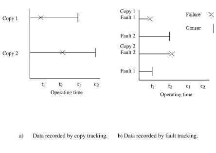
Figure 1 presents two different data representations. For simplicity, it is assumed
there are two copies (labeled 1, and 2) of the repaired item, although in general there
is no limit to the number of copies. Each copy is observed for different lengths of
(pre-determined) time denoted by c1, and c2 respectively. It is assumed that the item
contains two faults which are realized as failures at times t1, and t2, by copy 1, and 2
respectively. Figure 1a shows a failure history of the ‘fleet’ of copies by tracking the
history of each, while Figure 1b is the corresponding representation of the realization
of the faults & censoring times.
It is assumed that each copy of the item is identical with respect to the faults
they possess, and the nominal operating environment; and that each copy operates
independently of the other. Further, it is assumed that each copy began observation at
time 0 with the same K faults, and that once a particular fault is realized it is removed
from all copies. Moreover, we assume that distinctly different faults fail
independently of one another. We denote the number of copies in operation at time t
by U(t), and let
t be the rate of occurrence of failures for one copy at time t.These assumptions are consistent with a birth process with intensity function
, , 0,1, 2,...,F
i t U t t K i K i K
(1)
which describes the rate of occurrence of failure for the set of all copies, given i faults
have been realized.
The resulting probability distribution describing the number of faults realized
in the interval (t,t+ s) has a Binomial distribution of the form in Equation (2), where
--
-Pr
-1- , 0,...,
-t s t s
t t
n K i n
U y y dy U y y dy D t s D t n D t i
K i
e e n K i
n
(2)
Parametric inference under such censoring can result in optimistic estimates of
the reliability function due to the assumptions underlying the probability model [11].
The nonparametric approach to inference provides an alternative. For example, it is
trivial to calculate a Kaplan-Meier estimate [12] of the underlying distribution once
the data have been converted to a form represented in Figure 1a. However, the
construction of confidence intervals is not necessarily straightforward. Standard
approaches, such as Greenwood’s formula [12], rely on the Central Limit Theorem; and if the required large sample sizes are not achieved, these approaches can result in
confidence intervals for the reliability function that exceed 1, or fall below 0.
The use of bootstrapping for obtaining confidence intervals based on the
Kaplan-Meier estimate of the reliability function is well documented [13]. However
difficulties arise in adequately modeling the censoring structure using such an
approach. For simpler data structures, for example, where fault realization times are
censored independently of the realizations from other copies, re-sampling directly
from the Kaplan-Meier estimate [14] can result in asymptotically incorrect results
[15] as opposed to re-sampling directly from the data [16]. Therefore, we can
reasonably expect similar problems for the more complex censoring structure of
interest in this paper, where the sample size is varying throughout the period of
observation because copies are censored at different times. Therefore, we require
both means of estimating the reliability function for our scenario before we can
3. ESTIMATOR OF THE RELIABILITY FUNCTION
We begin by defining the reliability function for the probability that a particular fault
is not realized in the interval (0,t), assuming there is only one copy of the item. This
function provides information about how long a fault can remain within the item if it
were left to fail without interference from modifications, and is given by
0 -t u du R t e
(3)
We extend this reasoning to develop an estimator of the reliability function
under the assumed censoring structure using the approach of Kaplan Meier. Consider
the situation where Uj copies of the item are in operation at time tj,where ti represents
the time of the ith fault realization. Assume each copy contains K faults at the start of
operation, because all parts began observation at the same calendar time. If, at time ti,
the ith fault is realized, then K-i faults will remain within the item design. Once a fault
is exposed in one copy, it is removed from all copies without the addition of another
fault into the item design. Hence, an estimator of the conditional reliability function,
R(t|ti-1), is given by the ratio of the number of faults that will not have been realized
by time ti to the total number of faults that either remain undetected at time ti or are
realized by time ti
^
-1
1- -1
1-KM
i i i
i
U K i
R t t
K i U
(4)
The estimator of the unconditional reliability function is then the product of the
conditional reliability functions
^
1
- 1 -1
- 1
i j KM i
j j
U K j
R t
K j U
The proposed estimation procedure would be unbiased if the reliability function is
compiled from data collected at controlled discrete points selected along the
observation period because this would be based on modeling the number of faults
observed within any section of the observation period through a Binomial sampling
scheme. However, because we propose to estimate the reliability function at each
time a fault is realized, this will result in a bias. For example, consider the reliability
function conditional on survival to time ti-1, R(t|ti-1), where t< ti,. If at time t there are
Ui copies being observed that will also be observed at time ti, then there are K+ 1-i
faults remaining within the design. Denote the probability that a particular fault is not
realized by time t, given it has not been realized by time ti-1, as RF(t|ti-1) where the
subscript F is used to denote that there are a ‘fleet’ of copies. RF(t|ti-1) will be the
product of the conditional reliability functions for each copy, and so the probability
that a fault remains within a copy by time ti, given it was not realizes by time ti-1, is
given by
1-1 -1 Ui
i i F i i
R t t R t t (6)
At time ti-1, there are K-i faults remaining in the item, and there are Ui copies
being observed, all of which possess each fault. The distribution of the time to realize
the next fault, Ti, can be derived from an order statistic argument [17]. The time to
realization of the next fault will be the minimum fault realization time from a sample
of K+ 1-i, where each fault realization time is i.i.d. from the distribution with
reliability function RF(t|ti-1). The pdf of the time to realize the ith fault, given the
(i-1)th fault was realized at time ti-1, is
1-
-1 -1 -1
2 - K i , 0 , , ,
i F i F i i
Therefore, an unbiased estimator of the conditional reliability function at time ti would be
-1 1 ^ -1 -1 11--1 1- -1 -1
1-1 1-i i i U
i i F i i
K i U
F i i F i i F i i
t
i R t t E R t t
R t t K i R t t dR t t
K i K i U
(8)The estimator Equation (8) will always produce an estimate of reliability
which is greater than Equation (4) for the following reasons. The difference will
decrease as the number of copies increases, or when many faults remain within the
item design.
^ -1 ^ -1 1- -1 1-1 1-1 1 1 1 1- 1-1 iKM i i i
i i
i
i i
U K i
R t t K i U
K i
R t t
K i
U
K i U K i U
The conditional probabilities in Equation (8) lead naturally to the following estimator
for the reliability function
^ 1 - 1 1 - 1 i i j j K j R t K j U
(9)As each of the conditional reliability estimates given by Equation (8) are
unbiased & conditionally independent at each fault realization time, then Equation (9)
is an unbiased estimator of the underlying reliability function.
The bootstrap method of constructing confidence intervals is based on the principle of
strong repeated sampling, and is assessed by examining the behavior of the estimates
through hypothetical repetitions under the same conditions under which the data were
observed [18]. As such, data are simulated from the estimated reliability function
subject to both types of censoring: deterministic censoring of the copies, and random
censoring at the times at which faults are realized.
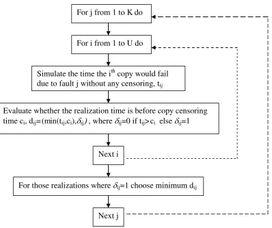
Figure 2 illustrates the modeling process. A natural approach to re-sampling would
be to simulate a realization time for each fault on each copy using
^R t . This would
require KU0 simulations. For each simulated realization time, there will be an
assessment of whether the fault was realized prior to the censored time of the copy.
This would require KU0 evaluations. For each fault, the earliest time it was observed
is recorded, and provides the re-sampled data from which the reliability function can
be re-estimated. This process is repeated indefinitely, and allows the variability in
estimation to be recorded & used to determine bootstrap confidence intervals. In
total, there will be 2MKU0 calculations, where M is the number of bootstraps required.
The re-sampling process described in Figure 2 would be simple to code.
However it is possible to develop an algorithm for calculating the bootstrap
confidence interval requiring fewer simulations with only 2MK calculations. This not
only reduces computational time, but also supports an explicit representation of the
confidence intervals.
To develop the revised algorithm, again we begin by assuming only one copy
is being observed for a pre-determined time cm. Consider the probability distribution
describing the time until a particular fault, say j, is realized; and denote this random
^ ^
1 1 1
Pr Tj ti R ti 1 R ti ti , c ti ti 0
(10)
The probability that a censored time for fault j is generated is given by
^PrTj cR c (11)
Because the two components of the right hand side of Equation (10) are conditionally
independent, we obtain an unbiased estimate of the probability of detecting a fault at
time ti+ 1.
When two or more copies are observed, the model needs to be extended to
include the random censoring mechanism. Therefore consider the distribution for the
time until fault j is first realized across all copies, and denote this random variable by
Xj. This distribution can be obtained from Equation (10), adjusting for the varying
number of copies being observed, and is given by
-1
-1 ^ ^ ^
-1 1
1
Pr m m i i , 0
i
U U U U
j i m i i i i
m
X t R t R t R t c t t
(12)If cmax represents the maximum censored time across all copies, then the
probability that fault j is censored from the fleet data is
-1 ^max
1
Pr m m
K
U U
j m
m
X c R t
(13)However, this leads to a bias in re-sampling for the following reasons. It has
been argued that the reliability function in Equation (9) is an unbiased estimator of the
reliability function at each time of fault realization, ti. As such, the successive ratios
between this estimator & the reliability function form a martingale process [18].
However, the re-sampling proposed in Equation (12) is a power transformation of the
successive ratios between Equation (12) & the true probability for this process would
form a sub-martingale process. Simply, we would have the following relationship
^
, 1,....,
U U
i i
E R t R t for i K
An unbiased re-sampling proportion would be obtained by using
1 max
1
Pr , : ,..., ,
1
j K
X x where x t t c
K
(14)
Assuming the realizations of distinctly different faults are independent
processes, the bootstrap re-samples for the realizations of the K faults can be
simulated from a multinomial distribution, with equal proportion assigned to each
realization time, or maximum censored time.
Bootstrap re-samples are generated from the data by conditioning on the
censoring times of the copies. Because there are K faults realized at times ti (i = 1 to
K), then the result from a re-sample will be a vector of fault realization times (x1,..,xk).
If the re-samples can be re-conceptualized as fixed times, where the number of faults
assigned to that time as their first realization are randomly selected, then we introduce
Ni to represent the number of faults assigned to time ti for time of first realization.
The vector of Ni (i=1 to K+1) has the following multinomial distribution
1 1 1 max
1 1
1 1
! 1
Pr ,..., ,
!... ! ! 1
,
K
K k K
K K
K i i
K
N n N n N c
n n n K
n K K
(15)
Having simulated the bootstrap data from the distribution in Equation (15), the
reliability function can be re-assessed. However re-sampling from a discrete
distribution in Equation (9) means it is possible that more than one fault can be
the bootstrapped data, it is no longer appropriate to use the approach in Equation (9);
but instead, one should employ the usual Kaplan-Meier for the conditional reliability
function
^ -1 -1 -1 -1 -1 -1 -1-i i i i
B i i
i i
i i
i i
U K D t D t t
R t t
U K D t
D t t
U K D t
(16)
where D(ti|ti-1) represents the number of faults realized at time ti, and D(ti-1) represents
the number of copies observed in the interval (0, ti-1]. Thus, the estimates of the
reliability function from the bootstrap data are computed from
^ -1 1 -1 1 -i j j B ij j j
D t t R t
U K D t
(17)5. EVALUATION OF THE BOOTSTRAP
The bootstrap confidence intervals are evaluated by comparing the expectation, and
the standard deviation of the conditional reliability function obtained through
bootstrapping, with those of the true reliability function.
5.1 Expectation of the Bootstrap Re-samples
From Equation (17), the re-sampled probability assigned to time ti can be considered
as a function of two correlated random variables, D(ti|ti-1) & D(ti-1), whose joint
distribution is
-1 - -1-1 -1 -1
-1 -1
! -1 1
1-Pr ,
! ! - ! 1 1 1
i i i i
d n K d n
i i i i i
i i i i
K i K i
D t d D t t n
d n K n d K K K
Repeated samples are taken from a birth process, which can terminate at each
of the observed order statistics, ti. Therefore, from Equation (18), we note that if all
faults were realized before time ti, then the reliability function at time ti would be
indeterminate. To overcome this problem, consider the expectation conditional on
there being faults to realize at the given times.
The expectation of each conditional probability assigned to the fault
realization times within the bootstrap can be derived from Equation (18) as
-1 -1 -1 ^ -1 -1 --10 0 -1 -1 -1
-1
! -1 1
1
- ! ! - ! 1 1 1
1--1 1 1 1 1 12
-i i i i
i
i i
B i i i
d n K d n
K d K
i
d n i i i i i i
K
i
E R t t D t K
n K i i
U K d d n K n d K K K
i K
U K i
(20)Hence, Equation (16) is clearly a biased estimator of the reliability function at
time ti. There are two obvious approaches to correcting for bias. One is to
arithmetically adjust the estimates by adding a corrective term, as shown in Equation
(21), and it is denoted by RBA. Alternatively, the conditional estimates can be adjusted
multiplicatively, as shown in Equation (22), and it is denoted by RBM. Each approach
would produce unbiased estimates, although RBM would also affect the variation,
which would increase with time.
-1
-1 1
1- 2 - 1
ˆ
-2 - 1- 1
i
i i
BA i i
i i
i
K i U K i
U n
R t t
U K d
K i U K i
(21)
-1 -1 1 ˆ 1 -1 1 11-1- 2
-i BM i i
i i
i i
n R t t
U K d
U K i U K i
Inspection of Equations (21) & (22) indicates that the bias will decrease as the
number of copies increases. The bias also increases as a function of t, such that bias
is greatest at tk, the time of the last fault realization.
5.2 Standard Deviation of the Bootstrap
Consider the variability associated with the conditional reliability function, firstly by
examining the standard deviation of the underlying stochastic process, and secondly
from the bootstrap re-samples before making a comparison.
Assume that immediately after time ti-1 there are K-D(ti-1) faults remaining,
and there are Ui copies being observed. An order statistic argument leads to a closed
form solution
-1 -1 2 -2-1 1 -1 -1 -1 -1
2
--1 -1
,.., -1
1-1- 2 1-2 1-2 1-i i i i K i U
i i i F i i F i i F i i
t
K i U
F i i F i i
i t
i
i
E R t t D t D t K R t t K i R t t dR t t
K i
K i R t t dR t t
U K i U K i K i U
Similarly, from Equation (8), we have
-1
1
-1
1-,.., -1
1
1-i i i
i
K i
E R t t D t D t K
K i U Therefore,
-1 1 -1
2 2
-1 1 -1 -1 1 -1
2
,.., -1
,.., -1 ,.., -1
1-
1-2 1
1-
1-i i i
i i i i i i
i i
Var R t t D t D t K
E R t t D t D t K E R t t D t D t K
K i K i
K i K i
U U (23)
-1 1 -1 2 ,.., 1- 1-2 1 1-
1-i 1-i i
R t t D t D t
i i
K i K i
K i K i
U U (24)
The bootstrap conditional reliability functions, are conditionally mutually
independent [19], hence we can derive the following expression for the variance.
2 1 -1 1 -1 -1 1- 1,.., 1 1
- 2 - 1-
-i i
i
j
i i i j
n K i
Var D t D t
U K d U K i K j K D t
(25)Therefore, an estimate of the standard deviation of
^-1 BA i i
R t t is given by
Equation (26), and for
^-1 BM i i
R t t by Equation (27). These expressions have been
obtained by substituting D(tj-1) with K+ 1-j, which is the E[D(tj-1)] .
-1 1 -1
2 1
ˆ ,..,
1- 1
1 1
2 -
1-BA i i i
i
j
R t t D t D t i
K i
K i K j
U
(26)
-1 1 -1
2 1
ˆ ,..,
1- 1
1 1
2 -
1-1 1
1
1-1- 2
-BM i i i
i
j
R t t D t D t
i
i i
K i
K i K j
U
U K i U K i
(27)The standard deviation from both adjusted bootstraps can be compared with
the order statistic approach in Equation (24). The calculations were based on fleet
sizes (U) ranging from 1 to 1000 copies, and the number of faults within the item
design (K) ranging from 5 to 501. Note that an odd number of faults were selected to
simplify the evaluation of the median. We found that the differences between
Equations (25) & (26) were negligible; therefore, only the results using Equation (26)
The maximum difference increases as the number of faults increases, while the
median difference, and the smallest difference both decrease. The number of copies
has a greater impact on the differences, whereby an increase in the number of copies
by a factor of 10 approximately decreases the difference by a factor of 10. In
summary, for situations where at least 10 copies are being observed, the differences in
standard deviations were small, and to all extents & purposes, negligible.
6. ILLUSTRATIVE EXAMPLE
This example is motivated by the development of complex electronic
equipment for aerospace systems. These data have been desensitized, but the key
messages associated with the application of the method are representative of actual
experiences. The item of equipment being developed was a variant of earlier
designs for which there was accumulated operating experience in similar
environments. Elicitation of engineering judgment was conducted to assess the
potential faults within the new design [20] based on the processes discussed in [4] and
historical data provided the duration of operating time until a fault is detected within a
copy of the item.
For an earlier generation of the design, 15 faults were realized over a period of
2 years. There were 20 copies in-service, of which half were censored after the first
year of operation, and the remainder after the second year. Each copy was exposed to
approximately 6000 operating hours per annum. Once a fault was realized in
operation, a modification was implemented across the fleet; this was assumed to occur
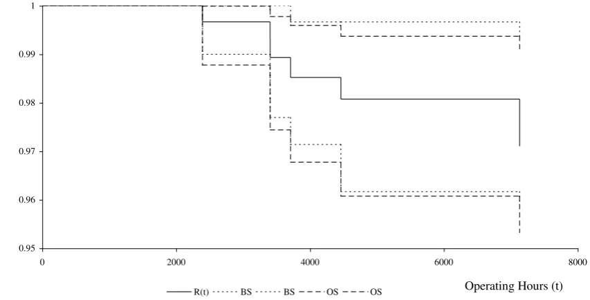
instantaneously. The estimated reliability function was calculated using Equation (6),
and is illustrated for the first year of operation in Figure 3, with 95% bootstrap
order statistic approach. Due to the high number of censored faults, the increments on
the reliability function are small, and at the end of the observation period, there is still
a high chance a fault would remain within the item without resulting in a failure.
We used Monte Carlo methods to simulate the number of faults exposed at each of the
fault realization times. At each time, the 2.5th and 97.5th percentiles were identified to
provide the 95% bootstrap point-wise confidence intervals. For the first year, there is
very little difference between the two sets of confidence intervals. Computations for
the order statistic confidence intervals for the second year are more challenging
because the fleet size changes. The largest deviation between the two sets of
confidence intervals occurs about 7000 hours with the difference on the lower bounds
being 0.00592.
The preferred methodology for constructing confidence intervals prior to the
development of the procedures presented in this paper would have been based on the
use of Greenwood’s formula. For this example, as expected, these approximate
intervals are consistently wider than the bootstrap point-wise, and the order statistic
confidence intervals, although the difference is not statistically large.
There are two main advantages for using bootstrap rather than analytical
solutions. First, as the number of copies changes throughout the observation period,
the calculations required to derive confidence intervals increases substantially.
Second, the bootstrap approach easily supports the determination of a confidence
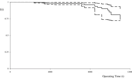
region for the reliability function. For example, Figure 4 illustrates the 95%
confidence region, together with the point estimate, of the reliability function. This
region is bounded by the two curves that contain 95% of the bootstrap reliability
functions. Figure 4 shows that the point estimate is very close to the lower bound of
the birth processes prior to the end of the observation period. Finally, an important
characteristic of these birth processes is that they do not possess independent
increments; therefore the usefulness of point-wise confidence intervals is limited.
6.1 Discussion
Assuming all copies begin observation at the same time, contain the same number of
faults, which when identified in any one copy are corrected, instantly & perfectly,
across all copies is unrealistic. For example, typical problems giving rise to
sequences of failure times for multiple copies of repaired items include aircraft fleet
reliability monitoring, warranty analysis of consumer goods such as mobile phones,
and plant-wide analysis of common components. In many cases, it may be that the
copies build up over calendar time giving rise to different exposure times, and
different numbers of inherent faults at any age. Our approach is adaptable to such
situations.
For example, if we have fleet data where the entry into service dates vary for
each copy, then this not only affects the exposure of faults to operating conditions but
some younger copies may be released into service with fewer faults than older copies
due to modifications implemented prior to their release. However, we assume that the
realization of faults is i.i.d. for each fault. As such, Equation (14) is a valid approach
for simulating the first realization of each fault, but Equation (16) requires correction.
The first necessary amendment is to record the calendar time of the realization
of each fault. Denote the calendar time of the realization of fault i by zi. The first
stage of the bootstrapping is to simulate the operational time of the first realization of
Equation (28). The operational time, ti, is associated with the copy that realized the
fault, and the index i is assigned to the ith smallest operational time.
1 max 11
Pr , , : 1,.., 1
1
j i i K K
X t z where i K t c z
K
(28)
From Equation (28), the number of faults that exist within each copy is evaluated as a
function of operating time; however, because copies enter service at different calendar
times, the number of faults per copy may differ. Denoting the number of faults
realized across the fleet by calendar time z as G(z), and the entry into service calendar
time of copy j by sj,then the number of faults in copy j after ti operating hours is
denoted by Yj(ti), and expressed as
0,
1 ,
j i j i
j i j i
if c t Y t
K G s t if c t
The conditional reliability function is estimated by
^-1 -1
1
1 i i
B i i U
j i j D t t R t t
Y t
(29)where D t t
i i-1
is the number of faults realized at time ti through the bootstrapsimulation. The overall reliability function is calculated as usual by evaluating the
products of the conditional reliability estimates.
REFERENCES
[1] J. Quigley, and L. Walls “Cost-Benefit Modelling for Reliability Growth,” Journal of Operational Research, 54, pp. 1234-1241, 2003.
[3] R. Cooke, and T. Bedford “Reliability Databases in Perspective,” IEEE Transactions in Reliability, 51, pp 294-310, 2002.
[4] L. Walls, and J. Quigley, “Eliciting prior distributions to support Bayesian reliability growth modelling –theory and practice,” Reliability Engineering and System Safety, 74, 2001, pp 117-128.
[5] W.R. Blishchke, and D.N.P. Murthy, Reliability: Modeling, Prediction and
Optimization, John Wiley, Chichester, 2000.
[6] M. Phillips, “Bootstrap Confidence Regions for the Expected ROCOF of a
Repairable System,” IEEE Transactions in Reliability, 49, pp 204-208, 2000. [7] H. Panjer, and G. Willmot, Insurance Risk Models, Society of Actuaries 1992.
[8] P. Boland, and H. Singh, “A Birth Process Approach to Moranda’s Geometric
Software Reliability Model,” IEEE Transactions in Reliability, 52, pp 168-174, 2003.
[9] B. Efron, and R. Tibshirani, An Introduction to the Bootstrap, Chapman and
Hall/CRC 1998.
[10] T. Seki, and S. Yokoyama, “Robust Parameter Estimation using the Bootstrap Method for the 2-Parameter Weibull Distribution,” IEEE Transactions in Reliability, 45, pp 34-41, 1996.
[11] J. Quigley, and L. Walls “Conditional Lifetime Data Analysis Using the Limited
Expected Value Function,” Quality and Reliability Engineering International,
20, pp 185-192, 2004.
[12] J. Lawless, Statistical Models and Methods for Lifetime Data 2nd Edition, John
Wiley, 2002.
[13] A. Davison, and D. Hinkley, Bootstrap Methods and Their Applications,
[14] N. Reid, “Estimating the Median Survival Time,” Biometrika, 68, 1981, pp. 601-608.
[15] M. Akritas, “Bootstrapping the Kaplan-Meier Estimator,” Journal of American Statistical Association , 81, 1986, pp 1032-1038.
[16] B. Efron, “Censored Data and the Bootstrap,” Journal of American Statistical Association, 76, 1981, pp.312-319.
[17] H.A. David, and H.N. Nagaraja, Order Statistics Third Edition, John Wiley
2003.
[18] S. Ross, Stochastic Processes 2nd Edition, John Wiley, 1996.
[19] D. London, Survival Models and Their Estimation, Actex Publications 1988.
[20] R. Hodge, M. Evans, J. Marshall, J. Quigley, and L. Walls L. “Eliciting Engineering Knowledge about Reliability During Design – Lessons Learnt from
a) Data recorded by copy tracking. b) Data recorded by fault tracking.
Figure 1: Representations of operational data with two censoring mechanisms.
Operating time Copy 1
Copy 2
Operating time Copy 1
Fault 1
Fault 2
Copy 2 Fault 2
Figure 2: Computationally intensive bootstrapping procedure. For i from 1 to U do
For j from 1 to K do
Simulate the time the ith copy would fail due to fault j without any censoring, tij
Evaluate whether the realization time is before copy censoring time ci, dij= (min(tij,ci),ij , where ij=0 if tij> ci else ij=1
Next i
For those realizations where ij=1 choose minimum dij
Figure 3: Comparison of point-wise bootstrap (BS), and true (OS) 95% confidence
intervals for reliability function for year 1 data. 0.95
0.96 0.97 0.98 0.99 1
0 2000 4000 6000 8000
Operating Hours (t)
R(t) BS BS OS OS
Figure 4: 95% confidence region for reliability function with point estimate of R(t) for
data from both years.
R(t)
0 0.25 0.5 0.75 1
0 4000 8000 12000
Table I:Bootstrap minus order statistic standard deviations of conditional reliability.
a) Maximum Difference.
K\U 1 10 100 1000
5 0.4306 0.0043 0.0003 0.000025
51 0.5184 0.0199 0.0019 0.000192
501 0.5281 0.0217 0.0021 0.000210
b) Median Difference.
K\U 1 10 100 1000
5 0.1643 0.0020 -0.0001 -0.00001
51 0.1004 0.0094 0.0009 0.00009
501 0.0406 0.0040 0.0004 0.00004
c) Minimum Difference.
K\U 1 10 100 1000
5 0.025800 -0.01416 -0.00260 -0.00028
51 0.000400 -0.00580 -0.00180 -0.00019
BIOGRAPHIES
John Quigley, PhD, CStat
Department of Management Science
University of Strathclyde
Glasgow G1 1QE, SCOTLAND
Email: [email protected]
John Quigley earned a BMath in Actuarial Science from the University of Waterloo,
Canada; and a PhD from the Department of Management Science, University of
Strathclyde, Scotland. Currently, he is a Senior Lecturer with research interests in
applied probability modeling, statistical inference, and reliability growth modeling.
He is also a Member of the Safety and Reliability Society, a Chartered Statistician,
and an Associate of the Society of Actuaries.
Lesley Walls, PhD, CStat
Department of Management Science
University of Strathclyde
Glasgow G1 1QE, SCOTLAND
Email: [email protected]
Lesley Walls is a Professor in Management Science, a Fellow of the UK Safety and
Reliability Society, a Chartered Statistician, and a member of IEC/TC56/WG2 on
reliability analysis. She holds a BSc in Applicable Mathematics, and a PhD in
Statistics. Her current research interests are in reliability modeling, and applied