AUTHOR’S POST PRINT (Romeo Colour: Green)
Int. J. Num. Meth. Fluids (ISSN: 0271-2091), 36 (1): 53-90 (2001). DOI: 10.1002/fld.120
Publisher version available at
http://onlinelibrary.wiley.com/doi/10.1002/fld.120/abstract
Three-dimensional numerical simulation of Marangoni
instabilities in liquid bridges: influence of geometrical
aspect ratio
M. Lappa
*, R. Savino and R. Monti
Università degli Studi di Napoli "Federico II"
Dipartimento di Scienza e Ingegneria dello Spazio "Luigi G. Napolitano", Università degli Studi di Napoli "Federico II", Napoli, Italy
*current e-mail address: marcello.lappa@strath.ac.uk
SUMMARY
Oscillatory Marangoni convection in silicone oil liquid bridges with different geometrical aspect ratios is investigated by three-dimensional and time-dependent numerical simulations, based on control volume methods in staggered cylindrical non uniform grids. The three-dimensional oscillatory flow regimes are studied and compared with previous experimental and theoretical results. The results show that the critical wave number (m), related to the azimuthal spatio-temporal flow structure, is a monotonically decreasing function of the geometrical aspect ratio of the liquid bridge (defined as ratio of the length to the diameter). For this function a general correlation formula is found, that is in agreement with the previous experimental findings. The critical Marangoni number and the oscillation frequency are decreasing functions of the aspect ratio; however, the critical Marangoni number, based on the axial length of the bridge, does not change much with the aspect ratio. For each aspect ratio investigated, the onset of the instability from the axi-symmetric steady state to the three-dimensional oscillatory one is characterized by the appearance of a standing wave regime that exhibits, after a certain time, a second transition to a travelling wave regime. The standing wave regime is more stable for lower aspect ratios since it lasts for a long time. This behaviour is explained on the basis of the propagation velocity of the disturbances in the liquid phase; for this velocity a general correlation law is found as function of the aspect ratio and of the Marangoni number.
Key words: liquid bridge, Navier-Stokes calculations, Marangoni flow.
1. INTRODUCTION
magnitude in space, surface tension-driven flows are the only mechanisms responsible for the appearance of undesirable instabilities in liquid semiconductors or other liquid melts materials during container-less floating zone crystal growth methods.
For a better understanding and optimization of these processes, model problems have been formulated and studied analytically, numerically and experimentally. The most common model is that of the half zone consisting of two circular, coaxial disks at different temperatures, with a bridge of liquid suspended between them. Since the end of 1970's (Chun and West1,2), on ground
experiments with small size half zones and high Prandtl number liquids (Pr>>1) pointed out that the Marangoni convection in liquid bridges heated from above or from below shows a transition from a steady axisymmetric toroidal flow to a three-dimensional oscillatory flow, when a critical temperature difference between the liquid bridge supports is exceeded. Preisser, Schwabe and Scharmann3, Velten, Schwabe and Scharmann4 and Frank and Schwabe5 performed
systematically on ground research over a large range of experimental conditions. They found that the oscillatory Marangoni flow exhibits different behaviour depending on the Prandtl number of the liquid employed and on the geometrical aspect ratio of the zone, defined as the ratio of the length L and of the diameter D of the bridge (A=L/D).
The onset of instability of Marangoni convection was investigated in space using large liquid bridges with length of the order of several centimeters and in absence of buoyancy effects by Monti6.
Experimental works have been performed recently on ground by Petrov et al.7, Muehlner et al.8,
Schwabe et al.9 .
In the last years the development of supercomputers and efficient numerical methods led the investigators to study the problem through numerical solution of the three-dimensional and time-dependent Navier Stokes equations.
Rupp, Mueller and Neumann10 studied by three-dimensional numerical simulations the
instability behaviour for different Prandtl number liquids and for a fixed aspect ratio (A=0.6). Stability analyses were carried out by several authors11-18,25 to define, in the non-dimensional
parameter space, sufficient conditions for stability and instability.
The most complete results on the subject are those reported in the linear stability analyses of Kuhlmann15 and Kuhlmann and Rath16 , Chen and Roux17 and Chen and Hu18. The basic
axisymmetric Marangoni flow was obtained by numerical solutions of the Navier-Stokes equations, together with the appropriate boundary and symmetry conditions, and the eigenvalue problem for the three-dimensional disturbances was solved over a range of Prandtl numbers and for aspect ratios close to unity. These results predicted the critical Marangoni numbers and the form of the most dangerous disturbances, characterized by the appropriate value of the critical wave number, in the neighbourhood of the neutral stability point (i.e., at the onset).
Kuhlmann and Rath16 found that the three dimensional supercritical state after the Hopf
The experiments performed on ground and in microgravity conditions revealed one or the other instability mechanism. For instance the travelling wave has been observed by Chun et al.1,
Preisser et al.3, Frank et al.5, Monti6,Muehlner et al.8 and Schwabe et al.9. The standing wave,
instead, has been observed during experimental ground-based activities (Velten et al.4, Frank et
al.5).
Recent numerical results obtained by Savino, Monti19 and Monti, Savino, Lappa20, have shown
that the standing wave and the travelling wave models correspond to two consecutive transitions of the Marangoni flow. In particular, for large Prandtl number liquids, the flow exhibits a first transition from the axi-symmetric steady to the three-dimensional oscillatory state, characterized by the standing wave instability and, after a certain time, a second transition from the standing wave to the travelling wave. These results, for a liquid bridge with a fixed aspect ratio (A=1), have been also validated by experimental results on ground (Monti, Savino, Lappa21) where, for
the first time the transition from one regime to the other was clearly observed.
In a previous work22 a parallel solution numerical method has been introduced and applied to
study three-dimensional Marangoni flow instabilities in liquids with low Prandtl number.
In this paper the method is extended to high Prandtl numbers for which most of the existing information comes from experiments and linear stability calculations. In particular the attention is focused on the influence of the aspect ratio on the flow instability, on the critical wave number (m) and on the spatio-temporal structures (pulsating or rotating).
2. PHYSICAL AND MATHEMATICAL MODEL
2.1 Basic assumptions
Fig.1 shows the geometry of the problem and the boundary conditions. A cylindrical liquid bridge is suspended between two coaxial disks with constant temperatures (T T O T/ 2), where T0 is the ambient temperature and T the overall temperature difference.
Th=Tc + T
z
r
u
v
v
Tc
The liquid is assumed homogeneous and Newtonian, with constant density and transport coefficients. The bridge is bounded by a cylindrical and undeformable liquid-gas interface with a surface tension exhibiting a linear decreasing dependence on the temperature:
=
o-
T(
T-
T0),
(1)where
o is the surface tension for TT0;
T is the negative rate of change of the surfacetension with temperature
(
T=-d
/d
T> 0).
The hypothesis of rigid free surface is acceptable if zero-g conditions prevail or, on the ground, if the volume of the liquid bridge is small and if the geometrical aspect ratio is sufficiently low.
2.2 Nondimensional field equations and boundary conditions
With the above assumptions the flow is governed by the continuity, Navier-Stokes and energy equations, that in non-dimensional conservative form read :
V 0 (2a)
V
t p VV Pr 2 V (2b)
T
t VT 2 T (2c)
where V, p and T are the non-dimensional velocity, pressure and temperature, Pr is the Prandtl number, defined by Pr=/ is the kinematic viscosiy and the thermal diffusivity). The non-dimensional form results from scaling the lengths by the axial distance between the circular disks (L) and the velocity by the energy diffusion velocity V = /L; the scales for time and pressure are, respectively, L/ and /L. The temperature, measured with respect to the
initial temperature T0 , is scaled by (T : )
T= (
T T 0) /
(T) (3)The initial conditions are:
t=0: V (z, r,
=0,
(z, r,
= 0
(4)i.e. the liquid is motionless and at ambient temperature.
on the cold disk
0 r R L/;
0 2V (z=0, r,
, t) = 0;
(z=0, r,
, t) = - 1/2
(5)on the hot disk
0 r R L/;
0 2V (z=1, r,
, t) = 0;
(z=1, r,
, t) = 1/2
(6)on the cylindrical free surface
0 z 1; 0 2
Vr (z, r=R/L,
, t) = 0
(7a)
Vr z r R L t Ma
T
z z r R L t
Z ( , / , , ) ( , / , , )
(7b)
r V
r
z r R L t V z r R L t Ma T z r R L t
( , / , , ) ( , / , , ) ( , / , , ) (7c)
T
r ( ,z rR L/ , , )t 0 (7d)
where the reference Marangoni number
Ma
is defined asMa=
T(T L/) .3. NUMERICAL SOLUTION
3.1 Solution method
The equations (2a-c) and the initial and boundary conditions (4-7) were solved numerically in cylindrical co-ordinates in primitive variables by a control volume method. The domain was discretized with a non uniform but structured axisymmetric mesh and the flow field variables defined over a staggered grid.
The axial velocity component Vz is staggered in axial direction with respect to the point in which temperature and pressure are computed. In a similar way the radial and azimuthal velocity components are staggered in radial and azimuthal directions respectively (see Fig. 2).
Fig. 2: collocation of the variables on the computational grid
see Figs. 3 where the projection (over a generic meridian plane) of the control volume Vz for the axial velocity, Vr for the radial velocity and p for the pressure and the temperature is shown (the control volumes for p, T are the same; the control volume for the azimuthal velocity V is shifted of an angular coordinate /2 in azimuthal direction with respect to the control volume used for P and T). Integrating over the generic control volume and using the Gauss theorem to transform volume integrals in surface integrals, the equations read
d n p t dS n V dS n V V t V V n n n 1 Pr 1 1 (8a)
n nn T t VT n dS T n dS
T
11 (8b)
The problem is solved with the well known Marker and Cell method (see e.g. Lappa and Savino22 and Fletcher23).
3.2 Validation of the numerical procedure
In this section the numerical model is validated by quantitative comparisons with 2D numerical results and with existing three-dimensional linear stability results for Prandtl numbers as close to that used in the present work as possible.
For two-dimensional computations, the stream function minimum of the axisymmetric flow in the case A=0.5, Pr=10 and Ma=1000 is compared with the results reported by Kuhlmann and Rath16 and Wanschura et al.25. Tables Ia and Ib show a very good agreement between the values
obtained with the present code and those by Kuhlmann and Rath16 and Wanschura et al.25
To check that the code is able to "capture" the physical instabilities of Marangoni flow, critical Marangoni numbers have been computed and compared with the results of two different available stability analyses. In particular the cases A=0.6 and Pr=10 (reported in the recent linear stability analysis of Chen and Hu18) and A=0.5, Pr=4 (reported in the linear stability analysis of
ijk
u
ijk
v
ijk
T
ij-1k
T
ij+1k
T
i+1jk
T
i-1jk
T
ij+1k
v
ij-1k
v
i-1j-1k
v
i-1jk
v
i+1jk
u
i+1j-1k
u
ij-1k
u
i-1j+1k
v
i-1jk
u
i-1j-1k
u
a)
ijk
u
ijk
v
ij+1k
u
ij-1k
u
i-1jk
u ui+1jk
ij+1k
v
i-1j+1k
v
i-1jk
v
b)
ijk
v
ijk
u
i+1j-1k
u
i+1jk
u
ij-1k
u
i+1jk
v
i-1jk
v
ij+1k
v
ij-1k
v
c)
Figs.3: control volumes adopted for the different variables
Regarding the definition of the critical conditions for the onset of instability, it is important to clarify the criterion adopted to evaluate so-called critical Marangoni number.
The linear stability analyses assume that the critical Marangoni number Mac is a threeshold value of Marangoni number at which the growth rate of the disturbances is zero. Typically, in these analyses the critical Marangoni number is computed using an extrapolation of the growth rate to zero.
For the present calculations, the critical Marangoni numbers have been defined as those for which the disturbance amplitude becomes vanishing (i.e. the non-dimensional azimuth velocity is of the order of 10-2), but is still characterized by a well-defined frequency. These values have
been determined using 3D simulation rather than extrapolation.
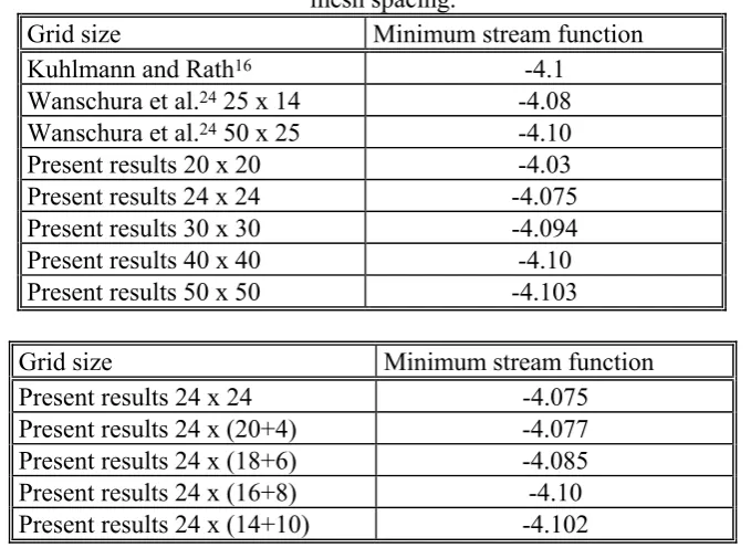
Table I: Minimum stream function of the axisymmetric flow as a function of mesh spacing.
Grid size Minimum stream function
Kuhlmann and Rath16 -4.1
Wanschura et al.24 25 x 14 -4.08
Wanschura et al.24 50 x 25 -4.10
Present results 20 x 20 -4.03
Present results 24 x 24 -4.075
Present results 30 x 30 -4.094
Present results 40 x 40 -4.10
Present results 50 x 50 -4.103
Grid size Minimum stream function
Present results 24 x 24 -4.075
Present results 24 x (20+4) -4.077
Present results 24 x (18+6) -4.085
Present results 24 x (16+8) -4.10
Present results 24 x (14+10) -4.102
The critical Marangoni number determined by the present numerical computations is Mac
13400 (3% greater that the linear stability value) with m=1 and a pulsating regime that is stable for a long time.
For Pr=4 and A=0.5 Wanschura et al.25 predict m=2 and Mac4200. The present results give
Mac4400 (5% greater that the linear stability value) and a pulsating regime that develops in a travelling regime after a short transient time.
These comparisons provides a sufficient validation of the present numerical code.
3.3 Grid refinement study
In this sub-section in order to show the numerical convergence of the present algorithm a grid refinement study is presented.
parameters P=1 and Q=2 have been used). This corresponds to a grid stretching factor not constant with a maximum value (max) for the layer of points adjacent the free surface.
Wanschura et al.25 found a change less than 1% in the stream function for a resolution of 25 x 14
points. In the present paper the same accuracy has been reached using uniform grids, for a resolution of 24 x 24 points.
Table Ib shows the results obtained with the present code using a grid size of 24 points in axial direction and a total of 24 points in radial direction. It can be seen that a non uniform mesh with 24 x (16+8) points gives the same accuracy as a uniform mesh with 40 x 40 points. This trend is confirmed by the behaviour of the axial component of velocity (at z=0.5 and different radial positions) shown in Table II.
A grid refinement study has been conducted also on the influence of the number of points used in azimuthal direction. In this case, the criterion for grid convergence is that the oscillation frequency changes less than 4%. The case A=0.5, Pr=4 and a supercritical situation (Ma=4800) has been considered to verify the accuracy of the simulation since it is expected that in this situation the numerical dissipation might be strong. Table IIIa shows that for the case A=0.5 grid convergence can be obtained using 20 points in azimuthal direction.
Table II: Axial velocity of the axisymmetric flow at z=0.5 and at different radial positions as a function of grid spacing (A=0.5, Pr=10, Ma=1000)
Grid size Vz at r=0.25 Vz at r=0.5 Vz at r=1.0
20 x 20 14.665 16.60 -43.83
24 x 24 14.59 16.624 -43.82
30 x 30 14.504 16.622 -43.80
40 x 40 14.44 16.605 -43.77
[image:9.595.212.418.518.671.2]24 x (16+8) 14.446 16.58 -43.79
Table III: 3D grid refinement study for (a) A=0.5, Pr=4, Ma=4800; (b) A=0.2, Pr=30, Ma=4.0 104
Grid size f
24 x (16+8) x 20 75.47 24 x (16+8) x 25 78.4 24 x (16+8) x 30 80
Grid size f10-2
4. RESULTS AND DISCUSSION
A parametric numerical analysis has been performed considering liquid bridges with different aspect ratios (from A=0.2 to A=0.7).
Due to the considerable computation time involved (each case requires a cpu time of the order of 100 cpu hours on a Silicon Graphics Power Challenge super computer) the investigation has been restricted to only one value of the Prandtl number (Pr=30, corresponding to a silicone oil with a kinematic viscosity =2 10-6 [m2/s]).
According to the grid refinement study, presented in the previous section, different non-uniform grids have been used to adequately meet the special features of the Marangoni flow in the liquid bridge. For high aspect ratios (A>0.5) the computational points have been distributed almost uniformly in the computational domain, whereas for low aspect ratios (A< 0.5) finer grids have been introduced near the free surface to enhance the resolution in the thin Marangoni boundary layer.
For A=0.7, 30 points have been collocated in the axial direction; this number has been reduced when reducing the length of the liquid bridge (24 for A=0.5 and 22 for A=0.2). In radial direction 30 points have been used in the case A=0.7 (no stretching and =1 everywhere), 24=16+8 for A=0.5 (max=1.1) and 28=14+14 for A=0.2 (max=1.2) (i.e the number of points
clustered near the free surface has been increased when the aspect ratio is decreased). In particular in azimuthal direction 20 points have been used for 0.4A0.7, 30 for 0.25A0.3 and 40 for A=0.2 (for this case a grid refinement study is shown in Table IIIb; the computed frequency shows grid convergence for N=25).
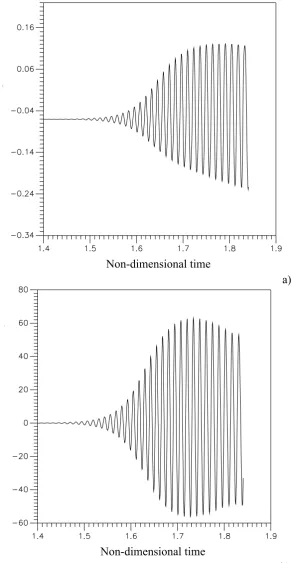
Fig. 4a shows the temperature profile at the point (z=0.75, r=0.5/2A, =0) for A=0.5 (Ma=3.5 104). The spatial symmetry of the flow breaks and a transient unsteady phase develops until a
stable supercritical oscillatory three-dimensional state is reached.
Very regular oscillations of the temperature are observed, with oscillation amplitudes increasing with time, until a fully established oscillatory regime (with constant maxima and minima) is reached.
This behaviour is in agreement with the previous stability analyses and with the experimental results that for large Prandtl number show that the onset of Marangoni instability develops as a Hopf bifurcation.
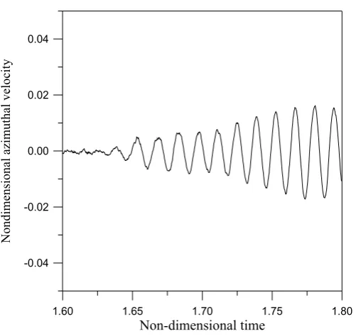
The oscillatory behaviour of the field is strictly correlated to the breaking of the space symmetry, since at the onset of the instability, an oscillatory azimuthal velocity component appears.
Fig. 4c shows the time-evolution of the azimuthal component of the velocity for Ma= 2.2 104; it
is very small (10-4 of the total velocity) and it increases with time with a very slow rate (very
close to zero). Fig. 4b shows the evolution of the azimuthal velocity for the same aspect ratio but for Ma=3.5 104. In this case the azimuthal velocity component is of the same order of magnitude
of the axial and radial components.
4.1 Description of the spatial organization in the supercritical state
F(z, r, , t) = Fo(z, r) + F~(z, r) sin (m ) (9)
where m is the azimuthal wave number that represents the number of spatial periods in the azimuthal direction. From a fluid-dynamic point of view this corresponds, for a fixed time, to a sinusoidal distortion of the section and of the axis of the three-dimensional Marangoni toroidal convection roll in azimuthal direction. The disturbances F~(z, r) may be imagined as a distortion wounded around the core of the toroidal vortex with a number of turns given by m.
To compare the present results with those obtained by previous stability analyses, the three-dimensional oscillatory disturbances were computed subtracting the azimuthally averaged flow [FO(z,r)] from the computed three-dimensional solution F(z,r,).
Table IV shows that the azimuthal wave number of the critical mode (m) is a function of the aspect ratio of the liquid bridge. In particular the critical number is m = 1 for A0.52, whereas higher values have been found for lower aspect ratios. Table IV shows that m = 1 for A 0.52, m = 2 for 0.3 A < 0.52, m = 3 for A = 0.25 and m=4 for A=0.2 (very short liquid bridge). The flow structure of the supercritical state is related to the value of m and hence depends on the value of the aspect ratio. Higher is m, more complex is the flow organization.
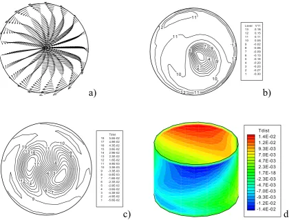
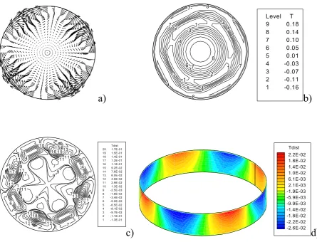
Figs 5,6,7,8 show for each aspect ratio the flow field in the cross-section orthogonal to the liquid bridge axis (a), the temperature distribution (b) and the temperature disturbances (c) in the same section and the temperature disturbances on the liquid bridge surface (d).
Figs. (a) show that in azimuthal direction there are 2m convective cells driven by the surface temperature distribution (d) (each surface spot has an angular extension of 360/2m degrees); Figs. (b) show that the isotherms of the supercritical state in the generic section z describe in this plane well defined curves whose shape is related to the value of the azimuthal wave number. For m = 1, as shown by Figs. 5 corresponding to the case A=0.7 and Ma=3.35 104, in the
generic cross-section orthogonal to the liquid bridge axis there are two azimuthal convective cells and two thermal spots in the section and on the liquid bridge surface; moreover the isolines of the temperature field in Fig. (b) permit to identify a lower temperature inner region whose shape is circular but whose position is eccentric to the geometrical axis of symmetry of the liquid bridge. In this case the supercritical flow appears as an inclined toroidal vortex (see Preisser et al.3). For m = 2 there are four convective cells and four thermal spots in the section and on the
free surface (two hot and two cold); the inner region in this case is not circular but approximately elliptic; this is shown in Figs. 6 corresponding to A=0.5 and Ma=3.5 104. This elliptic region has
axes e1 and e2 and is not eccentric but has centre corresponding with the geometrical axis of symmetry of the liquid bridge (see Fig. 6b). For m=3 and m=4 there are, respectively, six and eight vortex cells and surface spots, as shown in Figs. 7 for A=0.25, and Ma=3.8 104 and in Fig.
8 for A=0.2 and Ma=3.9 104. Moreover more complicated non eccentric patterns appear in the
Non-dimensional time
p
a)
Non-dimensional time
y
b)
[image:12.595.150.444.103.667.2]1.60 1.65 1.70 1.75 1.80 Non-dimensional time
-0.04 -0.02 0.00 0.02 0.04
No
ndimensio
nal azimuthal velocity
Figure 4 (continued)
The behaviour of the temperature field can be related directly to the nature of the disturbances. The temperature disturbances have m maxima (minima) in azimuthal direction (as shown in Figs. (c)). The nodes of the geometrical patterns described above simply correspond to these extrema in the temperature field. For m=2 the geometrical pattern is an ellipse since there are two minima and two maxima (in Fig. 6b the axes e1 and e2 connect respectively the axis of symmetry of the bridge with the positions corresponding to a minimum and to a maximum of the temperature disturbance distribution shown in Fig. 6c). For m=3 and m=4 the nodes correspond to the maxima of the disturbances.
[image:13.595.174.425.98.335.2]The radial position of the nodal lines of the temperature perturbations also corresponds to the position of the vortex centerline after the bifurcation.
Table IV: Mac versus geometrical aspect ratio
A Mac m f10-2 Vp10-2
0.2 2.45 104 4 11.36 8.91
0.25 2.4 104 3 7.38 7.72
0.3 2.35 104 2 5.17 8.12
0.4 2.3 104 2 3.08 4.83
0.5 2.2 104 2 2.77 4.35
0.52 2.17 104 1 2.4 7.54
0.55 2.15 104 1 2.25 7.06
0.6 2.1 104 1 2.0 6.28
[image:13.595.156.453.547.699.2]a)
4 5 6 7 8 9 9 10 10 1 1 1 1 1 1 1 2 1 2 1 2 1 3 1 3 Level V11 13 0.18 12 0.15 11 0.11 10 0.05 9 -0.02 8 -0.06 7 -0.09 6 -0.13 5 -0.16 4 -0.20 3 -0.23 2 -0.27 1 -0.30b)
3 6 6 7 8 8 9 9 10 10 11 12 13 14 16 1 7 Tdist 18 5.6E-02 17 4.9E-02 16 4.3E-02 15 3.6E-02 14 2.9E-02 13 2.3E-02 12 1.6E-02 11 9.8E-03 10 3.3E-03 9 -3.3E-03 8 -9.8E-03 7 -1.6E-02 6 -2.3E-02 5 -2.9E-02 4 -3.6E-02 3 -4.3E-02 2 -4.9E-02 1 -5.6E-02c)
Tdist 1.4E-02 1.2E-02 9.3E-03 7.0E-03 4.7E-03 2.3E-03 1.7E-18 -2.3E-03 -4.7E-03 -7.0E-03 -9.3E-03 -1.2E-02 -1.4E-02
d)
Fig. 5: (a) velocity field in the section z=0.5 for A=0.7, (b) temperature distribution, (c) temperature disturbances in the section z=0.75 for A=0.7 (d) temperature disturbance on the bridge surface for A=0.7 (Ma=3.35 104)
The present results pointed out (in agreement with previous experimental results1-3) that the
position of the vortex core is deformed and in particular displaced sinusoidally along the perimeter of the toroidal convection roll. This is due to the occurrence of additional convective cells in the sections orthogonal to the bridge axis (shown in Figs. 5a,6a,7a,8a), driven by the surface temperature spots (shown in Figs. 5d,6d,7d,8d), that convect fluid in azimuthal direction. The position of the vortex centerline describes in the space a sine curve having m maxima and m minima in the z-direction. The numerical simulations show that the part of the toroidal vortex that is displaced downwards is also displaced towards the centre of the zone and the part that is displaced away from the centre is at the same time displaced upwards (the displacement up and down is coupled to displacement out and in respectively). For this reason each plane orthogonal to the axis of symmetry shows temperature nodes that correspond to the intersection of the distorted vortex centerline with the considered plane.
[image:14.595.72.493.103.422.2]a)
1 23 4 5 6 8 8 9 1 0 1 0 1 1 1 1 1 2 1 3 1 3 1 4 1 4 1 5 15 15 1 5 1 6 1 6 1 6 1 6 1 71 7 1 7
17 1 8 1 8 1 8 1 9 Level V11 19 0.19 18 0.16 17 0.14 16 0.11 15 0.09 14 0.06 13 0.03 12 0.01 11 -0.02 10 -0.04 9 -0.07 8 -0.10 7 -0.12 6 -0.15 5 -0.17 4 -0.20 3 -0.23 2 -0.25 1 -0.28 e1 e2
b)
2 4 5 6 8 9 1 0 1 0 1 1 1 1 1 2 1 2 1 2 1 3 1 31 3 1 4
1 4 1 5 1 5 1 6 1 6 Tdist 18 1.2E-01 17 1.1E-01 16 8.9E-02 15 7.2E-02 14 5.5E-02 13 3.8E-02 12 2.0E-02 11 2.9E-03 10 -1.4E-02 9 -3.2E-02 8 -4.9E-02 7 -6.6E-02 6 -8.4E-02 5 -1.0E-01 4 -1.2E-01 3 -1.4E-01 2 -1.5E-01 1 -1.7E-01
c)
Tdist 3.6E-02 2.9E-02 2.3E-02 1.6E-02 9.8E-03 3.4E-03 -3.1E-03 -9.5E-03 -1.6E-02 -2.2E-02 -2.9E-02 -3.5E-02 -4.2E-02
d)
Fig. 6: (a) velocity field in the section z=0.5 for A=0.5, (b) temperature distribution, (c) temperature disturbances in the section z=0.75 for A=0.5 (d) temperature disturbance on the bridge surface for A=0.5 (Ma=3.5 104)
Wave numbers m = 1 and m = 3 belong to the class of "asymmetrical" modes; m = 2 and m = 4 are instead "symmetric" modes. More generally, when the critical disturbance number (m) is odd, there are two asymmetrical vortex cells in each meridian plane of the liquid bridge.
[image:15.595.70.504.100.424.2]a)
1 1 1 1 2 3 3 3 3 4 4 5 5 6 6 6 7 7 7 8 8 8 9 9 10 10 10 10 10 11 11 12 12 13 13 Level T 13 0.21 12 0.17 11 0.14 10 0.10 9 0.07 8 0.03 7 -0.00 6 -0.04 5 -0.07 4 -0.11 3 -0.14 2 -0.17 1 -0.21b)
1 3 4 4 5 5 5 6 7 7 7 7 8 8 9 9 9 1 0 1 1 1 0 1 1 1 1 11 1 2 1 3 1 3 1 3 1 4 Tdist 18 1.7E-01 17 1.5E-01 16 1.3E-01 15 1.2E-01 14 1.0E-01 13 8.2E-02 12 6.5E-02 11 4.7E-02 10 3.0E-02 9 1.2E-02 8 -5.3E-03 7 -2.3E-02 6 -4.0E-02 5 -5.8E-02 4 -7.5E-02 3 -9.3E-02 2 -1.1E-01 1 -1.3E-01c)
Tdist 3.4E-02 2.9E-02 2.3E-02 1.7E-02 1.2E-02 5.9E-03 2.4E-04 -5.5E-03 -1.1E-02 -1.7E-02 -2.3E-02 -2.8E-02 -3.4E-02d)
Fig. 7: (a) velocity field in the section z=0.5 for A=0.25, (b) temperature distribution, (c) temperature disturbances in the section z=0.75 for A=0.25 (d) temperature disturbance on the bridge surface for A=0.25 (Ma=3.8 104)
For even critical wave numbers, the flow field structure is on the whole three-dimensional and depends on the azimuthal co-ordinate, but in each axial plane the velocity and the temperature fields are symmetric and the time-dependence is observed as a synchronous pulsation of the two symmetrical vortices.
The different behaviours of the velocity field in a meridian plane, depending on the critical wave number (even or odd) are shown in Figs. 10,11,12 and 13 for two moments in time corresponding to the minimum and the maximum of the velocity oscillations during one cycle respectively.
[image:16.595.71.504.100.435.2]a)
1 1 1 2 2 3 3 4 4 4 5 5 5 6 6 6 7 7 7 7 8 8 8 9 9 Level T 9 0.18 8 0.14 7 0.10 6 0.05 5 0.01 4 -0.03 3 -0.07 2 -0.11 1 -0.16b)
2 3 3 4 4 4 5 6 6 7 7 7 7 7 7 8 1 0 9 9 9 1 11 1 9
9 9 1 1 1 1 1 1 1 1 1 1 1 3 1 2 1 3 1 3 1 3 1 3 1 5 1 6 1 7 1 8 1 9 Tdist 20 1.7E-01 19 1.5E-01 18 1.4E-01 17 1.2E-01 16 1.1E-01 15 9.2E-02 14 7.6E-02 13 6.0E-02 12 4.5E-02 11 2.9E-02 10 1.3E-02 9 -2.5E-03 8 -1.8E-02 7 -3.4E-02 6 -5.0E-02 5 -6.5E-02 4 -8.1E-02 3 -9.7E-02 2 -1.1E-01 1 -1.3E-01
c)
2.2E-02 1.8E-02 1.4E-02 1.0E-02 6.1E-03 2.1E-03 -1.9E-03 -5.9E-03 -9.9E-03 -1.4E-02 -1.8E-02 -2.2E-02 -2.6E-02 Tdistd)
Fig. 8: (a) velocity field in the section z=0.5 for A=0.2, (b) temperature distribution, (c) temperature disturbances in the section z=0.75 for A=0.2 (d) temperature disturbance on the bridge surface for A=0.2 (Ma=3.9 104)
The situations for A=0.25 (m=3) and A=0.2 (m=4) are illustrated in Figs.12 and 13 respectively. The liquid bridge in this case is very short and the two driving cells are confined near the free surface, with other counter-rotating vortex cells induced by continuity in the interior of the bridge.
Similar results were obtained using 2D computations by Rybicki and Floryan24 who found, for
short bridges, the emergence of several layers of vortices, with the strength of each layer decreasing approximately exponentially with the distance from the surface.
[image:17.595.72.518.101.441.2]
a)
b)
c)
d)
e)
f)
[image:18.595.109.449.103.507.2]
g)
h)
Figg. 9: streamlines of the projected velocity vectors on the meridian plane =0 for A=0.7 and Ma=3.35 104 (the field is shown in figs a,b,c,d,e,f,g,h corresponding to t=0, /8, /4, 3/8, /2, 5/8, 3/4, 7/8)
Table IV shows that, while the critical wavenumber changes with the aspect ratio, the critical Marangoni number does not change much and it is a smooth decreasing function of the aspect ratio of the bridge. This behaviour can be explained by the fact that when the aspect ratio decreases, the ratio of the free surface area Sl (where the "driving force" is present) divided by the end walls area Sw (where "no-slip" prevails), Sl/Sw=2A also decreases, increasing viscous effects and stabilizing the flow field.
On the other hand, the non dimensional frequency of the oscillations (f=fcD2/ where fc is the
computed critical frequency) strongly increases (Table IV).
Figg. 10: streamlines of the projected velocity vectors on the meridian plane =0 for A=0.7 and Ma=3.35 104 (the
field is shown in figs a,b corresponding to t=0, and t=/2)
Figg. 11: streamlines of the projected velocity vectors on the meridian plane =0 for A=0.5 and Ma=3.5 104 (the
field is shown in figs a,b corresponding to t=0, and t=/2)
Figg. 12: streamlines of the projected velocity vectors on the meridian plane =0 for A=0.25 and Ma=3.8 104 (the
field is shown in figs a,b corresponding to t=0, and t=/2)
Figg. 13: streamlines of the projected velocity vectors on the meridian plane =0 for A=0.2 and Ma=3.9 104 (the
4.2 Comparison with previous experimental and numerical results
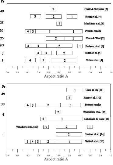
The critical wave numbers obtained for high Prandtl number liquids and different aspect ratios in previous studies are summarized in Table Va and Vb, that report, respectively, all the available experimental and numerical results. In both the tables the present numerical results are presented for comparison.
In particular (see Table Va), Chun et al.1,2 found experimentally m=2 mode for octadecane
(Pr=25) liquid bridge of small aspect ratio (A=0.45) and m=1 for A>0.5. Preisser et al.3 found
for NaNO3 zones (Pr=9.7) m=1 for A>0.65, m=2 for 0.4<A<0.65, m=3 for 0.25<A<0.4, m=4 for A<0.25 and the empirical relation 2mA2.1 between mode and aspect ratio, showing that the critical azimuthal wave number increases when the aspect ratio is reduced. For the same liquid Velten et al.4 found large ranges with modes m=2,3,4 around A=0.55, 0.375 and A=0.3
respectively; the product 2mA was found to have a value of 2.25 which is almost the same by Preisser et al.2.
In KCl melt (Pr=1) Velten et al.4 found instabilities with azimuthal component with m=2 around
A=0.6, m=3 around A=0.35 and m=4 around A=0.25 and 2mA2.1.
In liquid bridges of C24H50 (Pr=49) Velten et al.4 found m=2 near A=0.45, m=3 near A=0.32
and m=1 (not observed in KCl and NaNO3) near A=0.6 and 2mA1.8.
Muehlner et al.8 found m=1 for a liquid bridge of tetradecamethylhexasiloxane (Pr=35) for
A=0.5. Table Va shows that the present numerical results are in qualitative agreement with the previous experimental findings available for different values of the Prandtl number. In particular, these results satisfy the correlation function 2mA1.6 between the azimuthal wave number and the aspect ratio; the value 1.6 is almost the same obtained by Velten et al.4 for Pr=49.
Muehlner et al.8 used an infrared thermocamera with wavelengths centered at 4.61 m and
observed, for a Pr=35 and A=0.5, oscillatory Marangoni convection at Ma=13000 in the form of a travelling wave with m=1 (in contrast to the present results, that give, for Pr=30 and A=0.5, m=2 and Mac=22000). Concerning the apparent discrepancies between the experimental results reported by Muehlner et al.8 and the present numerical results a number of remarks can be
pointed out.
Muehlner et al.8 considered a non-cylindrical liquid bridge with a volume smaller than the
volume of the cylinder with same diameter and length (0.065 cm3, as reported in Ref.7 where the
same experiment of Muehlner et al.8 is described, in contrast to the cylindrical one 0.085 cm3).
In the present work a cylindrical zone has been investigated. This may explain the different results since, as well known and recognized by the same authors8 the critical conditions for the
onset of time dependence are sensitive to the volume. In fact as shown by Chen and Hu18 a 20%
change in volume can give rise to a 100% change in the critical Marangoni number. In addition, the present calculations show that the transition from m=2 to m=1 as the most unstable azimuthal wavenumber occurs for A0.52 and this together with the different shape of the bridge could explain the different azimuthal wave numbers.
Table Vb summarizes the previous numerical results. In particular Rupp et al.10 found m=2 for
A=0.6 and for Pr=49, but unfortunately, they did not make a study on the influence of the geometrical aspect ratio (A). Monti, Savino, Lappa20-21 found m=1 for A=1 and Pr=30 and
Table V: Critical azimuthal wave number versus the Prandtl number and versus the geometrical aspect ratio; comparison between the present numerical results and other available (a)
experimental results, (b) numerical and theoretical results
Aspect ratio A
Xu and Davis11 used linear-stability theory to determine sufficient conditions for instability to
infinitesimal disturbances for a half zone of infinite aspect ratio. They found that there is a critical value Pr* (50) of the Prandtl number such that if Pr<Pr*, the mode m=1 is preferred while if Pr>Pr* the mode m=0 is preferred. However, since they considered liquid bridges of infinite length their results cannot be directly applied to a finite-length liquid bridge.
Using energy stability theory Neitzel et al.13 found for a fluid of Prandtl number one a
monotonic cascade from m=5 to m=1 over the range 0.2<A<0.5 with m=1 persisting to A=0.9. Recently Yasushiro et al.28, using 3D computation have found for Pr=1 m=1,2,2 and 3 for
A=0.8, 0.65, 0.5 and 0.375 respectively.
In the linear stability results of Neitzel et al.14, for all cases considered (Pr=1 and 0.5<A<0.7)
the minimizing azimuthal wave number was m=2. These results agree with those obtained by Chen and Roux17 who found for a large range of Prandtl number and aspect ratios, m=2 as the
most critical wave number. These findings, however, do not agree with the results obtained in this work that show a dependence between the critical mode number m and the aspect ratio, according to the experimental observation by several investigators.
Chen and Hu18, using linear instability analysis, analyzed the influences of the aspect ratio (0.6
A1.4) and of the liquid bridge volume on the critical Marangoni number. They found m=1 as the most critical wave number for all the aspect ratios investigated and for Pr=1, Pr=10 and Pr=50 in agreement with the present results.
Kuhlmann and Rath16 performed a linear stability analysis over a large range of Prandtl
numbers. They found that for A=0.5 and 1<Pr<30 the most dangerous disturbances have wavenumber m=1. However there was some error in the calculations of Kuhlmann and Rath, which was discovered after the publication of their paper. In a more recent work (Wanschura et al.25) this error has been eliminated; for 0.8<Pr<5 they found m=2 for A=0.5. The same value
was found for A=0.5 by Neitzel et al.14 for Pr=1, and A=0.5, and in the present work for Pr=30.
4.3 Analysis of the oscillatory model: standing waves and travelling waves
The numerical results obtained in this work show that, for all the aspect ratios considered, the flow, immediately after the onset, may be properly described by the dynamic model of an "azimuthally standing wave". The three-dimensional temperature disturbance consists of a number m of couple of disturbances (hot and cold) “pulsating” at the same azimuthal positions along the interface and in the bulk (minimum and maximum disturbances at fixed azimuthal positions). These spots are responsible for thermocapillary effects in the azimuthal direction, causing 2m counter-rotating vortex cells in the transversal section.
After a second transition the instability mechanism becomes dominated by a travelling wave and the temperature spots rotate around the axis of the floating zone (the number of the spots depending on the aspect ratio as for the standing wave).
Figs. 14-15 show the temperature, and the vector plots in a transversal cross section for the standing wave regime and m=2 (A=0.4, Ma=3.6 104). The pulsating temperature spots on the
behaviour the convective cells in Figs. 15 change periodically their sense of rotation. Their intensity is not constant in time; if the considered convective cell is clock-wise oriented during the first half period, then during the second half of the period it vanishes and then reappears in the same azimuthal position anti-clock-wise oriented (Figs. 15).
The behaviour of the surface spots is also directly related to the motion of the toroidal vortex centerline. As explained in section 4.1 the position of the vortex centerline describes in the space a sine curve having 2 maxima and 2 minima in the z-direction (in the case m=2). During half period the maxima travel in z direction towards the cold disk and the minima travel in z direction towards the hot disk; in the second half the minima become maxima and vice versa.
2 3 3 3 4 4 4 5 5 6 7 7 8 8 9 9 1 0 1 0 1 0 1 1 1 1 1 1 1 2 1 2 1 3 1 3 1 4 1 4 e1 e2
a)
1 2 3 3 4 4 4 5 5 6 6 7 7 8 8 9 1 0 1 0 1 1 1 1 1 1 1 1 1 2 1 2 1 2 1 3 1 3 1 4 1 4 e1 e2b)
1 1 3 3 4 4 5 6 7 7 8 8 9 10 1 0 11 1 1 1 2 1 2 13 13 14 14 14 15 15 e1 e2
c)
1 2 3 4 5 5 5 6 6 6 7 8 9 9 1 0 9 1 1 1 1 1 2 1 2 1 2 1 2 1 3 1 3 1 4 14 e1 e2Level T 15 0.18 14 0.15 13 0.11 12 0.08 11 0.05 10 0.02 9 -0.01 8 -0.04 7 -0.08 6 -0.11 5 -0.14 4 -0.17 3 -0.20 2 -0.23 1 -0.27
d)
a)
b)
c)
d)
Figg. 15: Velocity field in the section z=0.5 for A=0.4 (Ma=3.6 104) and standing wave regime (the field is shown in figs a,b,c,d corresponding to t=0, /4, /2, 3/4)
Since the displacement up and down of the toroidal convection roll is coupled to displacement out and in respectively with respect to the axis of symmetry of the zone, this gives rise to an alternate expansion and contraction of the axes e1 and e2 of the elliptic inner region of the temperature field (Figs. 14). One complete period for this time-dependent behaviour takes a time 1/f where f is the characteristic frequency of the oscillations.
Figs.17-19 show the thermofluid-dynamic after the second transition to an azimuthally travelling wave. It can be observed that many differences exist with respect to the case of standing wave regime. In this case the behaviour is not "pulsating", but rotating.
a)
b)
c)
Tdist 3.6E-02 3.0E-02 2.4E-02 1.8E-02 1.3E-02 6.8E-03 1.0E-03 -4.8E-03 -1.1E-02 -1.6E-02 -2.2E-02 -2.8E-02 -3.4E-02 -4.0E-02
d)
Figg. 16: Temperature disturbance on the brige surface for A=0.4 (Ma=3.6 104) and standing wave regime (the field is shown in figs a,b,c,d corresponding to t=0, /4, /2, 3/4)
The standing wave regime for A=0.25 (m=3) and for A=0.2 (m=4) are depicted in Figs. 20-21 and Figs. 22-23 respectively. In this case the behaviour is similar to that described for the case m=2 the only difference being the different number of spots and vortex cells in azimuthal direction (Figs. 20 and 22 show a pulsation of the inner triangle and quadrangle respectively: the nodes of these polygons are replaced in time by the presence of sides and viceversa). One complete period for this time-dependent behaviour takes a time 1/f as in the case m=2.
2 3 4 5 5 6 7 8 9 9 10 10 11 11 12 12 12 13 14 14 15 15 16 16 17
a)
1 2 3 45 6 7 8 9 9 10 10 11 11 12 12 13 13 14 14 13 15 15 16 16 17b)
1 2 4 5 6 7 8 9 10 11 11 12 12 12 13 13 14 14 14 15 15 16 16 17 17c)
1 3 4 5 6 78 8 9 10 10 11 11 12 12 13 13 14 14 15 15 16 16 17 T 17 0.18 16 0.15 15 0.13 14 0.10 13 0.07 12 0.04 11 0.01 10 -0.02 9 -0.04 8 -0.07 7 -0.10 6 -0.13 5 -0.16 4 -0.18 3 -0.21 2 -0.24 1 -0.27d)
Figg. 17: Temperature distribution in the section z=0.75 for A=0.4 (Ma=3.6 104) and travelling wave regime (the field is shown in figs a,b,c,d corresponding to t=0, /4, /2, 3/4)
Although an azimuthally standing wave that develops in an azimuthally travelling wave after a certain time was observed for all the aspect ratios investigated, the standing wave model was found to be more stable for small aspect ratios. For 0.2<A<0.3 the standing wave regime lasts for a long time, whereas for A>0.3 the transition from the pulsating regime to the rotating regime occurs after a short transition time.
It must be emphasized that the azimuthal wave number and the fundamental frequency are independent of the type of oscillation (pulsating or rotating), so that it is not possible to identify the transition from one regime to the other using these values. However an other factor that can be considered a distinguishing mark between standing and travelling waves is the behaviour of the average Nusselt number on the cold and hot disks of the bridge.
The computations show that during the standing wave regime these average values are not constant in time but oscillate at a frequency that is double with respect to the frequency of the temperature oscillations.
a)
b)
c)
d)
Figg. 18: Velocity field in the section z=0.5 for A=0.4 (Ma=3.6 104) and travelling wave regime (the field is shown in figs a,b,c,d corresponding to t=0, /4, /2, 3/4)
This is shown in Fig. 24a. The Nusselt number oscillates with a frequency 2f during the pulsating regime but the amplitude of the oscillations decreases in time up to a constant value when the standing wave develops in travelling wave.
The decrease of the average Nusselt number can be explained on the basis of the amount of axial momentum that is converted in azimuthal momentum after the onset. The azimuthal momentum, in fact, does not contribute to the axial heat transfer near the disks.
a)
b)
c)
Tdist 3.6E-02 3.0E-02 2.4E-02 1.8E-02 1.3E-02 6.8E-03 1.0E-03 -4.8E-03 -1.1E-02 -1.6E-02 -2.2E-02 -2.8E-02 -3.4E-02 -4.0E-02
d)
Figg. 19: Temperature disturbance on the brige surface for A=0.4 (Ma=3.6 104) and travelling wave regime (the field is shown in figs a,b,c,d corresponding to t=0, /4, /2, 3/4)
This azimuthal mean flow, however has been found to be very small (in Fig. 24b for Pr=4 and A=0.5 the mean value of the azimuthal velocity is 10% of the amplitude whereas in Fig. 4b for Pr=30 and A=0.5 the mean value is 3% of the amplitude).
This is in agreement with the findings of Schwabe et al.9 who under supercritical conditions,
1 1 1 3 3 3 3 3 3 5 5 5 5 7 7 7 7 9 9 9 11 13 15 15
a)
1 1 3 3 3 3 5 5 5 5 7 7 7 7 9 9 9 9 9b)
1 1 1 1 3 3 3 3 5 5 5 5 5 7 7 7 7 7 9 9 9 11 11 13 13 13c)
1 1 3 3 3 3 5 5 5 5 7 7 7 7 9 9 9 Level V 15 153.92 14 141.13 13 128.34 12 115.55 11 102.76 10 89.97 9 77.19 8 64.40 7 51.61 6 38.82 5 26.03 4 11.26 3 0.69 2 -8.10 1 -17.18d)
Figg. 20: Radial velocity distribution in the section z=0.75 for A=0.25 (Ma=3.8 104) and standing wave regime (the field is shown in figs a,b,c,d corresponding to t=0, /4, /2, 3/4)
4.3.1 discussion
The computed spatio-temporal structures of the three-dimensional oscillatory Marangoni convection discussed above agree with those predicted by the previous linear stability analyses, according to which, for large Pr, the basic Marangoni flow loses its stability due to a pair of counterpropagating azimuthal waves, with a phase depending not only on and t but also on the radial and axial coordinates r and z.
The wave front F of such hydrothermal waves is inclined with respect to z. Since the constant-phase surfaces can be imagined as vertical planes that have been twisted around the vertical axis, the twist being given by a phase G(r,z), each wave having an amplitude A(r,z) can be represented according to Kuhlmann and Rath26 as:
( , )
exp ) ,
(r z i m t G r z
A
F (10)
A superposition of two counterpropagating waves with the same amplitude results in
a)
b)
c)
Tdist 3.4E-02 2.9E-02 2.3E-02 1.7E-02 1.2E-02 5.9E-03 2.4E-04 -5.5E-03 -1.1E-02 -1.7E-02 -2.3E-02 -2.8E-02 -3.4E-02
d)
Figg. 21: Temperature disturbances on the bridge surface for A=0.25 (Ma=3.8 104) and standing wave regime (the field is shown in figs a,b,c,d corresponding to t=0, /4, /2, 3/4)
Since in this case the oscillatory term does not depend on , maximum and minimum disturbances are fixed in space and the minimum is continually replaced by the maximum and viceversa as soon as cos(t-G(r,z)) changes its sign. These extrema in the disturbance distribution give rise to hotter and colder zone in the bridge and the three-dimensional temperature disturbance consists of a number m of couples of spots (hot and cold) pulsating at the same azimuthal positions along the interface.
When the amplitude of the two hydrothermal waves is not the same the superposition gives :
F A r z ( , ) (a m) cos (b m G, )t (11b)
(the functions a and b are reported in Ref.26) so that the oscillatory term depends on ; in this
case the minimum and maximum disturbances travel in the azimuthal direction and the phase of the oscillations depends continuously on .
1 1 1 2 1 3 3 4 3 3 3 5 5 5 5 5 7 7 7 9 9 9 11 11 13
a)
1 1 1 1 1 3 3 3 3 3 3 3 5 5 5 7 7 7 7 9 9 9 9 11 11b)
1 1 1 1 1 1 3 3 3 3 3 4 3 5 5 5 5 5 7 7 7 7 9 9 9 11 11 13c)
1 1 1 1 1 3 3 3 3 3 5 5 5 7 7 7 9 9 9 9 11 11 11 Level V 13 115.17 12 102.06 11 88.95 10 75.85 9 62.74 8 49.63 7 36.52 6 23.41 5 10.30 4 0.21 3 -1.04 2 -2.81 1 -7.30d)
Figg. 22: Radial velocity distribution in the section z=0.75 for A=0.2 (Ma=3.9 104) and standing wave regime (the field is shown in figs a,b,c,d corresponding to t=0, /4, /2, 3/4)
The linear stability theory cannot predict if the standing wave or the travelling wave instability prevails since the relative amplitude of the two counterpropagating azimuthal waves depends on non-linear effects; the present computations that are based on the solution of the complete and non-linear Navier-Stokes equations show that the travelling wave model appears after the standing wave regime (after a time that depends on the aspect ratio of the liquid bridge). Probably this behaviour can be explained by the fact that at the beginning two counter-propagating waves with equal amplitude are formed, while in a second phase one of these waves prevails over the other.
The azimuthally travelling wave has been observed by different investigators, either on ground or in microgravity (Ref.1-6,8,9).
Schwabe et al.9 used a stereo microscope (rather than a light cut technique) and observed in the
a)
b)
c)
2.2E-02 1.8E-02 1.4E-02 1.0E-02 6.1E-03 2.1E-03 -1.9E-03 -5.9E-03 -9.9E-03 -1.4E-02 -1.8E-02 -2.2E-02 -2.6E-02
Tdist
d)
Figg. 23: Temperature disturbances on the bridge surface for A=0.2 (Ma=3.9 104) and standing wave regime (the field is shown in figs a,b,c,d corresponding to t=0, /4, /2, 3/4)
Velten et al.4, measuring the temperature near the free surface by three thermocouples positioned
at the same radial coordinate but at different azimuthal positions, observed two different non-axisymmetric spatial structures of Marangoni convection: 1) running waves with an azimuthal component (corresponding to the travelling wave regime observed by other investigators); 2) axially running waves with deformed wave front. The latter regime corresponds to the standing wave regime, as demonstrated by Kuhlmann and Rath26.
Recently Frank et al.5 using a light cut technique observed clearly pulsating and rotating
regimes.
In the present paper the criterion to detect the regime (pulsating or rotating) has been based on the phase shift between two "numerical" probes located on the free surface at the same axial position with an angular shift of 90/m degrees. As discussed in section 4.1, each surface spot has an angular extension of 360/2m degrees. During the standing wave regime two cases are possible: 1) the two thermocouples are located on the same spot (the phase shift is 0); 2) the two probes are located on two adjacent different spots (the phase shift is ). When the regime is rotating the two probes give signals that show a constant phase shift related to the angular distance between them (for an angular shift of 90/m the phase shift is /2).
9.50 10.00 10.50 11.00 11.50 Non-dimensional time
4.60 4.62 4.64 4.66 4.68 4.70
Avera
ge
Nusselt nu
mber (hot
di
sk)
Standing wave regime Steady
Travelling wave regime
a)
9.50 10.00 10.50 11.00 11.50 12.00
Non-dimensional time
-20.00 -10.00 0.00 10.00 20.00
No
n-dime
nsional azi
mu
th
al velocit
y Standing wave regime
Travelling wave regime
Mean value
b)
Fig. 24: (a) Average Nusselt number on the hot disk in the case A=0.5, Pr=4, Ma=4800, (b) azimuthal velocity in the point z=0.75, r=0.5, =0 for A=0.5, Pr=4, Ma=4800.
[image:33.595.163.441.102.613.2]4.4 Disturbances propagation velocity
This section will be dedicated to the discussion of the results obtained for the different aspect ratios considered in the numerical analysis, on the basis of the concept of the azimuthal velocity of propagation of the disturbances and of previous experimental results reported in the literature. As discussed before, the transition from the standing wave regime to the travelling wave occurs after a short transition time if the aspect ratio is high whereas it is quite stable and prevails for a long time if the aspect ratio is low (see Fig. 25) .
This behaviour can be explained by the velocity of propagation of the hydrothermal disturbances in the liquid, since this velocity is a function of the aspect ratio and of the Marangoni number. In particular, the propagation speed of the travelling disturbances is defined as
m R
V~P 2 (12)
where R is the radius of the bridge, m the critical mode number and
the period of the oscillations.This velocity in non-dimensional form (see Table IV) reads:
f m D D m
R D
V
VP P
/ 2 ~
2
[image:34.595.72.444.367.686.2]* (13)
where *and f are the dimensionless period and the dimensionless frequency of the oscillations respectively .The propagation speed of the temperature disturbances is determined by the relative importance of the two contributions to the overall heat transfer (conduction and convection). Hence, it follows that the travelling speed of the azimuthal perturbation is proportional to the Marangoni number as pointed out by Chun et al.1.
In Ref.27 it has been found experimentally that the dimensionless frequency can be expressed
as:
2 / 3 3 / 2 2
2 / 1 2 / 3 3 / 2
2 1 2
1
k Ma L D D k Ma A
f
(14)
(where k depends on the Prandt number of the liquid: k0.7 for Pr=30) and substituting the (14) in the (13) it follows that
2 / 1 3 / 2
2
1
Ma A
mA
VP (15)
Since 2mA is almost constant (2mA=1.6) and since Mac does not change much with decreasing the aspect ratio, it is clear that the disturbance propagation speed increases with A-1/2 when A is
reduced.
From Table IV (Vp computed using (13)), it can be observed that the increase of the propagation speed of the travelling disturbances takes place mainly for 0.3<A<0.4.
The results discussed before have shown that the standing wave regime is more stable and that it lasts for a long time if the aspect ratio is lower than 0.3%0.4 .
Chun and West1 observed that the time-evolution of the flow after the onset should be related to
the growth and propagation of the temperature disturbances. According to their theory, the growth or the damping of a small temperature disturbance depends on the ratio of the rapidity of the heat transfers by conduction and by convection. For the extreme case of very high conductive heat transfer, a temperature disturbance should die diffusing very rapidly in all directions. On the other extreme case of very high convective heat transfer, the disturbances should move with the flow, "frozen" in the flow motion. Between these two extremas, the temperature disturbances which travel in different azimuthal directions with their own propagation velocity, should interfere with each other and be amplified in the progress of time.
According to Chun and West1 the velocity of propagation of the disturbances is a "critical
5. CONCLUSIONS
A numerical code based on a three-dimensional control volume method and able to use a non-uniform mesh has been developed which is able to give a three-dimensional and time-dependent simulation of Marangoni flow instability in cylindrical non isothermal liquid bridges.
Since most of the existing information for high Prandtl numbers comes from experiments and linear stability calculations, a high Prandtl number liquid (Pr=30) has been considered in the computations.
The numerical results have been analyzed and interpreted in the general context of the bifurcations theory.
The numerical calculations show, according to available experimental results and according to linear stability results, that lower is the aspect ratio higher is the critical wave number and more complex the flow field structure. The empirical correlation 2mA=1.6 between the azimuthal wave number and the aspect ratio has been found which is almost identical to that one obtained by several experimental investigators for high Prandtl liquid zones.
Owing to the cylindrical geometry of the floating zone two different modes for oscillatory flow pattern are principally possible, one being an asymmetric mode and the other a symmetric mode. The main criterion for the occurrence of symmetric or asymmetric modes is the aspect ratio. A characteristic feature of the asymmetric basic mode m=1 is a periodically "staggering ring" of vortex core of the toroidal flow pattern on a meridian section of the floating zone and also a periodically tilting branching streamline which divides the two vortices in the generic meridian plane. For the symmetric basic mode two vortices on the meridian plane are moving up and down simultaneously, and accordingly the tilting of the branching streamline disappears.
Standing wave and travelling wave regimes have been observed and depicted in detail.
In the pulsating regime the temperature disturbances "pulsate", i.e. the cold surface spots grow in axial direction during the shrinking of the hot spots and viceversa but the azimuthal positions of these extrema do not change. According to the presence of these surface spots convective cells are formed in the planes orthogonal to the liquid bridge axis, their number depending on the azimuthal wave number. These cells change periodically their sense of rotation and their intensity. The behaviour of the surface spots has been directly related to the motion of the toroidal vortex centerline whose shape is distorted in axial direction. The pulsating behaviour of the temperature field in the generic section has been explained considering that the displacement up and down of the toroidal convection roll is coupled to displacement out and in respectively with respect to the axis of symmetry of the zone.
The behaviour of the azimuthally travelling regime has been explained in detail too.
In this case the surface temperature spots do not change their intensity and rotate around the perimeter of the liquid bridge. The vortex cells in the section orthogonal to the axis do not change their sense of rotation and their strength is constant in time (the cells never vanish). The time dependent behaviour of the velocity field is simply characterized by a full rotation of the the entire flow pattern in azimuthal direction.
The numerical results pointed out that the transition from one regime to the other depends on the aspect ratio of the liquid bridge. In particular it was found that the azimuthal standing wave regime is more stable and lasts for a long time for low aspect ratios . Moreover thanks to the numerical simulation performed for A0.5, Pr=4, Pr=10 and Pr=30 it was possible to establish that the standing wave regime is more stable for high Prandtl numbers.
A detailed description of the disturbances and in particular of their azimuthal wave number, velocity of propagation and time of growth has been given.
The transition from pulsating regime to rotating regime has been explained in terms of the velocity of propagation of the disturbances in the liquid since this velocity is function of the aspect ratio and of the Marangoni number.
6. ACKNOWLEDGEMENTS
This work is part of the PhD thesis of M.Lappa.
The authors would like to thank the Italian Aerospace Research Center (CIRA) that allowed the numerical calculations on the Silicon Graphics Power Challenge Parallel Supercomputer.
7. REFERENCES
[1] C.H. Chun, W. West, "Experiments on the transition from the steady to the oscillatory Marangoni
convection of a floating zone under reduced gravity effect", Acta Astronautica 6, 1073-1082 (1979).
[2] C.H. Chun ,"Experiments on steady and oscillatory temperature distribution in a floating zone due to
the Marangoni convection", Acta Astronautica 7 ,479-488 (1980).
[3] F. Preisser, D. Schwabe, A. Scharmann, "Steady and oscillatory thermo capillary convection il liquid
columns with free cylindrical surface", J.Fluid Mech. 126, 545-567 (1983).
[4] R. Velten, D. Schwabe, A. Scharmann, "The periodic instability of thermocapillary convection in
cylindrical liquid bridges", Phys.Fluids A 3, 267-279 (1991).
[5] S. Frank , D. Schwabe, "Temporal and spatial elements of thermocapillary convection in floating
zones", Experiments in Fluids, 23, 234-251 (1998).
[6] R. Monti, "On the onset of the oscillatory regimes in Marangoni flows", Acta Astronautica 15,
557-560 (1987).
[7] Petrov V., Schatz M.F., Muehlner K.A., Van Hook S.J., McCormick W.D., Swift J.B., "Experimental control of thermocapillary convection in a liquid bridge", Third Microgravity Fluid Physics Conference NASA CP 3338, 487-492 (1996).
[8] K.A. Muehlner , M. F. Schatz , V. Petrov , W.D. McCormick , J.B. Swift , H.L. Swinney,
"Observation of helical traveling-wave convection in a liquid bridge", Phys. Fluids 9 (6) , 1850-1852
(1997).
[9] D. Schwabe , P. Hintz , S. Frank, "New Features of Thermocapillary Convection in Floating Zones Revealed by Tracer Particle Accumulation Structures", Microgravity sci. technol. 9, 163-168 (1996). [10] R. Rupp, G. Muller, G. Neumann, "Three dimensional time dependent modelling of the Marangoni
convection in zone melting configurations for GaAs", Journal of Crystal growth 97, 34-41 (1989).
[11] J.J. Xu. and S.H. Davis, "Convective thermocapillary instabilities in liquid bridges", Phys. Fluids
27, 1102-1107 (1984).
[12] Y. Shen Y., G.P. Neitzel, D.F. Jankowsky, H.D. Mittelmann, "Energy stability of the thermocapillary
[13] G.P. Neitzel., C.C. Law, D.F. Jancowski, H.D. Mittelmann, "Energy stability of thermocapillary
convection in a model of the float-zone crystal-growth process", Phys. Fluids A 3, 2841-2846 (1991).
[14] G.P. Neitzel., K.T. Chang, D.F. Jancowski, H.D. Mittelmann, "Linear stability of thermocapillary
convection in a model of the float-zone crystal-growth process", Phys. Fluids A 5, 108-114 (1992).
[15] H.C. Kuhlmann, "Thermocapillary instabilities in cylindrical liquid bridge", Proceedings VIIIth European Symposium on Materials and fluid Sciences in Microgravity Brussels (Belgium), 12/16 April 1992 , ESA SP-333, 79-83 (1992).
[16] H.C. Kuhlmann, H.J. Rath, "Hydrodinamic instabilities in cylindrical thermocapillary liquid
bridges", J.Fluid Mech. , 247 , 247-274 (1993).
[17] G. Chen, B. Roux , "Bifurcation analysis of thermocapillary convection in cylindrical liquid
bridges", ELGRA Meeting, Madrid, December 1994, ELGRA News 19, 54, June 1995.
[18] Q.S. Chen, W. R. Hu , "Influence of liquid bridge volume on instability of floating half zone
convection", Int. J. Heat Mass Transfer, 41, 825-837 (1998).
[19] R. Savino and R. Monti, "Oscillatory Marangoni convection in cylindrical liquid bridges", Phys.
Fluids, 8, 2906-2913 (1996)
[20] R. Monti, R. Savino, M. Lappa, "Oscillatory Thermocapillary flows in simulated floating zones with
time-dependent boundary conditions"; Acta Astronautica 41, 863-875, (1997).
[21] R. Monti, R. Savino, M. Lappa and R. Fortezza, "Scientific and Technological Aspects of a
Sounding Rocket Experiment on Oscillatory Marangoni Flow", Space Forum, 2, 293-318 (1998).
[22] M. Lappa, R. Savino, "Parallel solution of three-dimensional Marangoni flow in liquid bridges", Int.
J. Num. Meth. Fluids, 31, 911-925 (1999).
[23] C.A.J. Fletcher , "Computational techniques for fluid-dynamics", (Springer Verlag, Berlin, 1991)
[24] A. Rybicki, J.M. Florian, "Thermocapillary effects in liquid bridges. I. Thermocapillary convection",
Phys. Fluids, 30, 1956-1972 (1987).
[25] M. Wanschura, V. Shevtsova, H.C. Kuhlmann, H.J. Rath, "Convective instability mechanism in
thermocapillary liquid bridges", Phys. Fluids A 5, 912-925 (1995).
[26] H.C. Kuhlmann, H.J. Rath, "On the interpretation of phase measurements of oscillatory
thermocapillary convection in liquid bridges", Phys. Fluids A 5 (9) 2117-2120 (1993).
[27] R. Monti et al., "First Results from 'Onset' Experiment during Spacelab Mission D-2", Proceedings of the Norderney Symposium on Scientific Results of the German Spacelab Mission D2, Editors P.R. Sahm, M.H. Keller, B. Schiewe, 247-258 (1995).
[28] S. Yasushiro, T. Sato , N. Imaishi, "Three dimensional oscillatory Marangoni flow in half-zone of