Rochester Institute of Technology
RIT Scholar Works
Theses Thesis/Dissertation Collections
2-1-2009
Face recognition with variation in pose angle using
face graphs
Sooraj Kumar
Follow this and additional works at:http://scholarworks.rit.edu/theses
This Thesis is brought to you for free and open access by the Thesis/Dissertation Collections at RIT Scholar Works. It has been accepted for inclusion in Theses by an authorized administrator of RIT Scholar Works. For more information, please [email protected].
Recommended Citation
Face Recognition with Variation in Pose Angle
Using Face Graphs
by
Sooraj Kumar
A Thesis Submitted in Partial Fulfillment of the Requirements for the Degree of Master of Science in Computer Engineering
Supervised by Dr. Andreas Savakis
Department of Computer Engineering Kate Gleason College of Engineering
Rochester Institute of Technology Rochester, NY
February 2009
Approved By:
_____________________________________________ ___________ ___
Dr. Andreas Savakis, Professor and Department Head
Primary Advisor – R.I.T. Dept. of Computer Engineering
_ __ ___________________________________ _________ _____
Dr. Muhammad Shaaban, Associate Professor
Secondary Advisor – R.I.T. Dept. of Computer Engineering
_____________________________________________ ______________
Dr. Juan Carlos Cockburn, Associate Professor
Acknowledgements
Abstract
Automatic recognition of human faces is an important and growing field. Several real-world applications have started to rely on the accuracy of computer-based face recognition systems for their own performance in terms of efficiency, safety and reliability. Many algorithms have already been established in terms of frontal face recognition, where the person to be recognized is looking directly at the camera. More recently, methods for non-frontal face recognition have been proposed. These include work related to 3D rigid face models, component-based 3D morphable models, eigenfaces and elastic bunched graph matching (EBGM).
Table of Contents
Chapter 1 Introduction ... 1
1.1. Face Detection and Recognition ... 1
1.2. Challenges of Pose-invariant Face Recognition ... 3
1.3. Thesis Contribution ... 4
1.4. Thesis Outline ... 5
Chapter 2 Background ... 6
2.1. Active Shape Models ... 6
2.1.1 Point Distribution Model ... 7
2.1.2 Training the PDM Model ... 8
2.1.3 Initializing the ASM in the Image Frame ... 9
2.1.4 Calculating a Suggested Movement for Each Model Point ... 9
2.1.5 Using the PDM as the Local Optimizer for the Contour ... 12
2.1.6 Termination of Iteration under Suitable Condition ... 15
2.2. Gabor Wavelets, Jets and the Similarity Function ... 16
2.3. Elastic Bunch Graph Matching ... 18
2.3.1 Face Representation ... 20
2.3.2 Face Recognition ... 25
Chapter 3 Automatic Feature Point Positioning ... 27
3.2. Automatic Placement Scheme ... 29
3.2.1 Correcting Face Image Alignment ... 30
3.2.2 Find the best-fit locations of fiducial points ... 32
3.3. Evaluation of the procedure... 37
Chapter 4 Feature Weighting and Face Derotation... 40
4.1. Face Recognition Using Elastic Bunch Graph Matching... 41
4.2. Feature Weighting Scheme ... 42
4.2.1 Motivation ... 42
4.2.2 Procedure ... 43
4.2.3 Evaluation of Weighted Recognition Scheme ... 49
4.3. Face Derotation Scheme ... 54
4.3.1 Motivation ... 54
4.3.2 Procedure ... 56
4.3.3 Evaluation of Derotation Results ... 62
Chapter 5 Pose-invariant Face Recognition with Jet-Mapping ... 66
5.1. Motivation ... 66
5.2. Procedure ... 67
5.2.1 Study of Jet Coefficients ... 67
5.2.2 Suggesting a Mapping... 69
5.5. Evaluation of the Combined Recognition Scheme ... 77
Chapter 6 Conclusions and Future Works ... 83
6.1. Summary of works ... 83
6.1.1 Automatic Feature Point Positioning ... 83
6.1.2 Feature-Weighted Recognition Scheme ... 83
6.1.3 Face Derotation Scheme ... 83
6.1.4 Jet-Mapped Recognition Scheme ... 84
6.1.5 A Combined Recognition Scheme ... 85
6.2. Scope for Possible Future Work ... 86
6.2.1 Training for Face Derotation ... 86
6.2.2 Improving Automatic Feature Point Placement ... 86
6.2.3 Real-Time Implementation ... 86
List of Figures
Figure 1 An example of a Shape Model. ... 7
Figure 2 Sampling Points along the Contour Normal ... 10
Figure 3 Finding the Best-Fit estimates along the Normal ... 11
Figure 4 Applying Displacement Constraint ... 15
Figure 5 A 2D Gabor Wavelet ... 16
Figure 6 A Model Graph ... 19
Figure 7 A Bunch Graph ... 20
Figure 8 Fiducial Points and the Face Graph structure ... 21
Figure 9 Displacement Estimation ... 24
Figure 10 A Face Image with locations of features given as priori information ... 29
Figure 11 Block Diagram illustrating Automatic Feature Point Positioning ... 30
Figure 12 3D Rotation components: Yaw, Pitch and Roll. ... 31
Figure 13 Face Alignment Process ... 32
Figure 14 The Different ASM Shapes Used ... 33
Figure 15 Fitting the ASM to extract the required graph node positions ... 34
Figure 16 Face Graphs Used for Different Face Poses ... 35
Figure 17 Finding best fit points around the Eyes ... 36
Figure 18 Finding Lip Corner By Finding the Steepest Edge in the neighborhood ... 36
Figure 19 Performance of Automatic Feature Point Positioning in comparison with Manually Selected Nodes ... 38
Figure 22 Face Similarity at different face poses. ... 44
Figure 23 Weighted Recognition Scheme ... 44
Figure 24 Feature Weights calculated for different pose graphs. ... 47
Figure 25 Recognition Rates for Weighted Recognition scheme ... 53
Figure 26 An illustration for the concept of Derotation ... 55
Figure 27 Illustration for the Concept of Derotation ... 56
Figure 28 Control Graphs ... 58
Figure 29 Mapping of Control Points ... 58
Figure 30 Derotation Process ... 60
Figure 31 Comparison of the Derotated Face to the Face in Library ... 61
Figure 32 Derotation Exampes ... 65
Figure 33 Distributions of selected Jet Coefficients for two different poses ... 69
Figure 34 Block Diagram illustrating Jet-Mapped Recognition Scheme ... 70
Figure 35 Effect of Jet-Mapping on selected Coefficients ... 71
Figure 37 Block Diagram illustrating Combined Recognition Scheme ... 76
List of Tables
Table 1 Description of the Feature Points used in recognition ... 35 Table 2 Calculation of weights for 15°, 30° and 45° Face Pose Graph ... 48 Table 3 Evaluation Results for Weighted Face Recognition scheme using Manually
Positioned Feature Points for 15° Face Pose Query Images ... 51 Table 4 Evaluation Results for Weighted Face Recognition scheme using Manually
Positioned Feature Points for 30° Face Pose Query Images ... 51 Table 5 Evaluation Results for Weighted Face Recognition scheme using Manually
Positioned Feature Points for 45° Face Pose Query Images... 50 Table 6 Evaluation Results for Weighted Face Recognition scheme using Automatic
Feature Points Positioning for 15° Face Pose Query Images ... 51 Table 7 Evaluation Results for Weighted Face Recognition scheme using Automatic
Feature Points Positioning for 30° Face Pose Query Images ... 52 Table 8 Evaluation Results for Weighted Face Recognition scheme using Automatic
Feature Points Positioning for 45° Face Pose Query Images ... 52 Table 9 Evaluation Results for Derotated Face Recognition scheme using Manual Feature
Points Positioning for 22° Face Pose Query Images ... 63 Table 10 Evaluation Results for Derotated Face Recognition scheme using Manual
Feature Points Positioning for 22° Face Pose Query Images ... 63 Table 11 Evaluation Results for Jet-Mapped Face Recognition scheme using Manually
Table 13 Evaluation Results for Jet-Mapped Face Recognition scheme using Manually Positioned Feature Points for 45° Face Pose Query Images ... 73 Table 14 Evaluation Results for Jet-Mapped Face Recognition scheme using Automatic
Feature Point Positioning for 15° Face Pose Query Images ... 73 Table 15 Evaluation Results for Jet-Mapped Face Recognition scheme using Automatic
Feature Point Positioning for 30° Face Pose Query Images ... 73 Table 16 Evaluation Results for Jet-Mapped Face Recognition scheme using Automatic
Feature Point Positioning for 45° Face Pose Query Images ... 74 Table 17 Calculation of Weights for Jet-Mapped Face Pose Graphs ... 78 Table 18 Evaluation Results for Jet-Mapped Face Recognition scheme using Manually
Positioned Feature Points for 15° Face Pose Query Images ... 79 Table 19 Evaluation Results for Combined Recognition scheme using Manually
Positioned Feature Points for 30° Face Pose Query Images ... 80 Table 20 Evaluation Results for Jet-Mapped Face Recognition scheme using Manually
Positioned Feature Points for 45° Face Pose Query Images ... 80 Table 21 Evaluation Results for Jet-Mapped Face Recognition scheme using Automatic
Feature Point Positioning for 15° Face Pose Query Images ... 80 Table 22 Evaluation Results for Combined Recognition scheme using Automatic Feature Point Positioning for 30° Face Pose Query Images ... 81 Table 23 Evaluation Results for Jet-Mapped Face Recognition scheme using Automatic
Glossary
Term Definition of the term as used in the thesis
ACM Active Contour Model ASM Active Shape Model
EBGM Elastic Bunch Graph Matching
Face Library A repository of frontal face images of known identities that are used for face recognition.
Model Face Image A frontal face image in the face library.
Query Face Image A face image without pose constraints that is to be recognized by matching with images into the face image library.
Face Profile The vertical line that divides the face into two roughly symmetrical parts.
Face Profile Plane The vertical plane passing through the vertical axis and the face profile line.
Pose Angle Geometric angle made by the intersection of the face profile plane and the vertical plane normal to the camera image plane. Face Detection Finding a face in an image.
Face Recognition Identifying the individual by comparing a given face to known, or trained, faces present in the Face Library.
Chapter 1
Introduction
1.1. Face Detection and Recognition
Face Recognition is an important and ever-growing area of interest in the field of Computer Vision. This is a classification problem, where known faces of several individuals are ‘trained’ beforehand by feature extraction, and upon introduction of a new, unclassified face, the individual from the library of ‘trained’ individuals is to be identified.
Face recognition systems typically consist of two basic steps. The first step involves detecting the face position on the image frame and identifying facial features of interest. The latter step involves extracting the facial information and using it to recognize the face across a library of pre-trained faces. Both steps are quite elaborate, and hence, have been considered as separate problems to be solved independently. However, the performance of the face detection step directly affects the face recognition step. Hence, it is still important that both steps be performed with as much accuracy as possible.
region, methods like Active Contour Models (ACMs) [5] are available for extracting local face feature regions based on standard face shapes.
The face recognition step can be chiefly divided into two broad categories: recognition by whole face, or recognition by components. Most of the basic principles behind face recognition can be developed from the understanding of human vision concepts [6]. Holistic face recognition methods, such as Principal Component Analysis-based eigenfaces [7] match the entire face.
Recognition by parts is implemented in approaches such as component-based face recognition with morphable models [8] and elastic bunched graph matching [9]. Modular eigenspaces [10] is an alternative approach to using eigenfaces. This methodology involves recognizing key components of the face individually and then piecing the recognized parts together to identify the face. Recognition by parts allows for a small amount of flexibility in the face structure, which is more robust.
1.2. Challenges of Pose-invariant Face Recognition
The human face is a three-dimensional structure, and its two-dimensional projection varies dramatically with respect to the point/plane of view, i.e. variation in face pose with respect to the image capturing device. This is a cause of concern for any recognition algorithm that relies solely on basic image processing techniques to find similarities between two-dimensional images, when there is disparity in the points of view between the two face images.
Face images in training databases are usually restricted to a very small set of known face poses. Most training is done only on frontal face poses and, in some cases, full-profile face poses. These poses are generally easy to obtain from the subjects. However, in an unconstrained environment, which is the case in real-world implementations of face recognition algorithms, the query face images are usually not in one of the trained face poses. This disparity in face pose, between the query and trained images, is the cause of significant reduction in recognition rates.
Gabor wavelets [13] are a prominent mathematical tool that can help describe features through a series of convolutions. Much research has been done using Gabor wavelet-based filters for frontal face recognition [14] [15], and some research pertaining to fixed-pose face recognition [9]. However, recognition across pose using Gabor wavelets has not been considered up to this point in time.
1.3. Thesis Contribution
This thesis considers the application of Gabor wavelets in pose-variant face recognition using Elastic Bunch Graph Matching as the base recognition system. The thesis then implements different independent procedures in trying to improve the face recognition rate of the base system across face pose variation and studies the robustness of each procedure towards face pose variation.
Considering the fact that the human face is almost symmetric along the vertical center, this thesis focuses only on pose variation along one direction, and assumes that a similar set of procedures can be applied for pose variation in the opposite direction as well. All experiments are carried out on faces gradually rotated in pose in an anti-clockwise direction.
The major contributions of this thesis are as bulleted below:
• An automated procedure for extracting essential feature points corresponding to facial features, using a few heuristics, is introduced and considered as a basis for face recognition.
• Another novel approach to improving pose-variant face recognition using Gabor jets, called Jet Mapping, is proposed and the performance results are studied.
1.4. Thesis Outline
Chapter 2
Background
This chapter reviews previous methods that are being implemented in this thesis work. Section 2.1 explains the concept of Active Shape Models, which is relevant in finding object contours in images. Active Shape Models are used later in Chapter 3 to support the Automatic Feature Point Positioning scheme. Section 2.2 covers the basics involved in performing recognition using Gabor wavelets and jets. This is further used throughout this thesis as a basis for recognition, and is modified as needed in each scheme that is introduced in Chapters 4 and 5. Section 2.3 also covers the implementation of a face recognition scheme called Elastic Bunch Graph Matching, which uses Gabor wavelets and jets, described in Section 2.2, as its basis for recognition.
2.1. Active Shape Models
2.1.1 Point Distribution Model
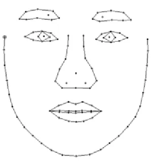
The Point Distribution Model (PDM) [17] helps generate a statistical representation of the contour points of shapes that fit different objects of the same class. This is based on the assumption that all of the shapes being represented have a flexible shape model of labeled nodes, over which controlled deformations can be applied to generate each individual shape, within a small margin of error. The necessary equations used in this thesis are reproduced in this section.
[image:19.612.231.380.298.458.2]
Figure 1. An example of a Shape Model.
The model consists of the mean positions of the labeled points and the main modes of variation describing how the points tend to move from the mean;
𝒙𝒙=𝒙𝒙�+𝑷𝑷𝑷𝑷 (2.1)
where 𝒙𝒙 is the vector representing the positions of the 𝒏𝒏 points in the shape, and
𝒙𝒙= (𝑥𝑥0,𝑦𝑦0,𝑥𝑥1,𝑦𝑦1, …𝑥𝑥𝑘𝑘,𝑦𝑦𝑘𝑘, …𝑥𝑥𝑛𝑛−1,𝑦𝑦𝑛𝑛−1)𝑇𝑇
(𝑥𝑥𝑘𝑘,𝑦𝑦𝑘𝑘) represents the position of point 𝑘𝑘 in the shape, 𝒙𝒙� is a vector representing the
mean position of all the points, 𝑷𝑷= [ 𝒑𝒑1 𝒑𝒑2 … 𝒑𝒑𝑡𝑡] is a matrix of the first 𝑡𝑡 modes of
Component decomposition of the position variables, and 𝑷𝑷 = (𝑏𝑏1 𝑏𝑏2 … 𝑏𝑏𝑡𝑡)𝑇𝑇 is a
vector of weights for each of the 𝑡𝑡 modes. The columns of 𝑷𝑷 are orthogonal. So
𝑷𝑷𝑇𝑇𝑷𝑷= 𝑰𝑰
and from Equation (2.1):
𝑷𝑷=𝑷𝑷𝑻𝑻(𝒙𝒙 − 𝒙𝒙�) (2.2)
The mean shape 𝒙𝒙� and the modes of variation 𝑷𝑷 are calculated from a set of training examples. Equation (2.2) can be used to estimate the weights 𝑷𝑷 needed to generate a shape from the model that can best fit a given shape 𝒙𝒙.
Equation (2.1) allows the generation of new shapes from the class of shapes, by varying the parameters (𝑏𝑏𝑖𝑖) within suitable limits. We can define the shape of a model
object by just choosing the values of 𝑷𝑷. An instance 𝑿𝑿 of the model can be placed in an image frame, by defining a scale, orientation and position transform for the model, as in the following equation:
𝑿𝑿= 𝑀𝑀(𝑠𝑠,𝜃𝜃)[𝒙𝒙] + 𝑿𝑿𝑐𝑐 (2.3)
where 𝑿𝑿𝑐𝑐 = (𝑋𝑋𝐶𝐶 𝑌𝑌𝐶𝐶 𝑋𝑋𝐶𝐶 𝑌𝑌𝐶𝐶 … 𝑋𝑋𝐶𝐶 𝑌𝑌𝐶𝐶)𝑇𝑇, 𝑀𝑀(𝑠𝑠,𝜃𝜃)[ ] is an operation defining
rotation by 𝜃𝜃 and scaling by 𝑠𝑠, and (𝑋𝑋𝐶𝐶,𝑌𝑌𝐶𝐶) is the new center of the model in the image
frame coordinates.
2.1.2 Training the PDM Model
the training set. Cootes et al [17] outline the process of standardizing a given set of shape models in order to obtain the best PDM model.
2.1.3 Initializing the ASM in the Image Frame
The pose and shape parameters of the ASM have to be initialized before any of the computations can be performed. Normally, the pose parameters would have to be initialized to arbitrary values, such that the ASM model is placed within a close proximity of the object in the image, so that the ASM can converge to the object contour. Wei Wang et al [18] propose using salient features, which can be easily located with good accuracy using automated detectors, to initialize the shape model and provide region constraints on the subsequent iterative shape searching.
2.1.4 Calculating a Suggested Movement for Each Model Point
2.1.4.1 Edge Constraint in Local Texture Model Matching
Local Texture Model Matching, as proposed by [18], makes use of the Mahalanobis distance function to estimate the best texture match position at each model point. However, this thesis shall utilize a simple least distance approach for finding the best texture match position along the normal of each point, as described below.
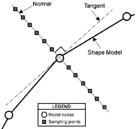
The texture model at a point in the shape model is the one-dimensional array of grayscale texture value sampled at 2𝐾𝐾+ 1 points along the normal to the contour, with 𝐾𝐾
[image:22.612.180.451.305.562.2]points extending on either side of the contour shape, as illustrated in Figure 2.
Figure 2. Sampling Points Along the Contour Normal.
A texture model 𝑔𝑔𝑖𝑖𝑖𝑖, which is a vector of 2𝐾𝐾+ 1 grayscale samples, is generated
for the 𝑖𝑖𝑡𝑡ℎ contour point in the 𝑖𝑖𝑡𝑡ℎ training model. The set of texture models {𝑔𝑔
𝑖𝑖𝑖𝑖} at all
estimating the best texture match positions in calculating a suggested movement for each model point in an iteration.
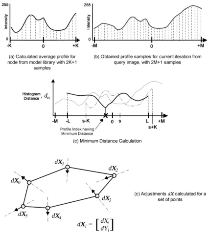
To find the best texture match position along a normal to a model point, we first have to sample 𝑀𝑀 points along the contour points’ normal on either side of the contour, totaling to 2𝑀𝑀+ 1 grayscale samples, where 𝑀𝑀 >𝐾𝐾. For the 𝑠𝑠𝑡𝑡ℎ sampling point along
the normal, −𝐿𝐿 ≤ 𝑠𝑠 ≤ 𝐿𝐿;𝐿𝐿= (𝑀𝑀 − 𝐾𝐾), a window of 2𝐾𝐾+ 1 texture samples is taken from the sampled set of 2𝑀𝑀+ 1 values, centered at the 𝑠𝑠𝑡𝑡ℎ sampling point, as illustrated
in Figure 3, and the distance 𝑑𝑑𝑖𝑖𝑠𝑠 between the texture model 𝑔𝑔𝑖𝑖𝑠𝑠 of the current window
and the average node texture model 𝑔𝑔̅𝑖𝑖 is calculated.
𝑑𝑑𝑖𝑖𝑠𝑠 = � �𝑔𝑔𝑖𝑖(𝑠𝑠−𝑝𝑝)− 𝑔𝑔̅𝑖𝑖(𝑠𝑠−𝑝𝑝)�
𝐾𝐾
𝑝𝑝=−𝐾𝐾
, −(𝑀𝑀 − 𝐾𝐾)≤ 𝑠𝑠 ≤(𝑀𝑀 − 𝐾𝐾)
This is done for all the 2(𝑀𝑀 − 𝐾𝐾) + 1 sampling points along the normal of each model point 𝑖𝑖. Then, the sample point 𝑠𝑠 with the minimum texture distance 𝑑𝑑𝑖𝑖𝑠𝑠 for that
model point is considered to be the best fit position and the displacement to that sample point from the current model point position is taken as the suggested movement
(𝑑𝑑𝑋𝑋𝑖𝑖,𝑑𝑑𝑌𝑌𝑖𝑖) for that model point. The change in position of all the node points in the
contour with respect to the image frame, calculated during an iteration, is represented by a vector 𝑑𝑑𝑿𝑿, where
𝑑𝑑𝑿𝑿= (𝑑𝑑𝑋𝑋0,𝑑𝑑𝑌𝑌0,𝑑𝑑𝑋𝑋1,𝑑𝑑𝑌𝑌1 …𝑑𝑑𝑋𝑋𝑛𝑛−1,𝑑𝑑𝑌𝑌𝑛𝑛−1)𝑇𝑇.
2.1.5 Using the PDM as the Local Optimizer for the Contour
ASM makes use of the PDM of an object as a constraint on the final deformation of the active contour at the end of iteration. Suppose the change in position of each of the node points in the contour, calculated during an iteration, is represented by a vector 𝑑𝑑𝑿𝑿, where
The current locations of the points in the image frame, represented by 𝑿𝑿, have to be moved to their new positions 𝑿𝑿+𝑑𝑑𝑿𝑿. This is brought about by a controlled change in the pose and shape parameters used for generating 𝑿𝑿 from the PDM model.
If the current estimate of the model centered at (𝑋𝑋𝐶𝐶,𝑌𝑌𝐶𝐶), with scale 𝑠𝑠 and
orientation 𝜃𝜃, new values of these pose parameters have to be estimated to better fit the image with the current model. This is done by finding the translation (𝑑𝑑𝑋𝑋𝐶𝐶,𝑑𝑑𝑌𝑌𝐶𝐶), rotation
𝑑𝑑𝜃𝜃 and scaling factor (1 +𝑑𝑑𝑠𝑠) from 𝑑𝑑𝑿𝑿 according to the procedure outlined in [19]. Once the pose variables are adjusted, the remaining residual adjustment in the model shape 𝒙𝒙 is denoted as 𝑑𝑑𝒙𝒙. The residual adjustment needed 𝑑𝑑𝒙𝒙, has to be calculated in the object co-ordinate frame, so that:
𝑿𝑿+𝑑𝑑𝑿𝑿=𝑀𝑀(𝑠𝑠(1 +𝑑𝑑𝑠𝑠),𝜃𝜃+𝑑𝑑𝜃𝜃)[𝒙𝒙+𝑑𝑑𝒙𝒙] + (𝑋𝑋𝐶𝐶+𝑑𝑑𝑋𝑋𝐶𝐶) (2.4)
Equation (2.4) includes coordinates expressed in two different coordinate frames. The object model 𝑿𝑿 and the change 𝑑𝑑𝑿𝑿 are relative to the image coordinate frame, while the local object model 𝒙𝒙 and the local deformation 𝑑𝑑𝒙𝒙 are relative to the object coordinate frame. Solving for 𝑑𝑑𝒙𝒙 gives the following equation:
𝑑𝑑𝒙𝒙= 𝑀𝑀 ��𝑠𝑠(1 +𝑑𝑑𝑠𝑠)�−1,−(𝜃𝜃+𝑑𝑑𝜃𝜃)�[𝑀𝑀(𝑠𝑠,𝜃𝜃)[𝒙𝒙] +𝑑𝑑𝑿𝑿 − 𝑑𝑑𝑿𝑿𝐶𝐶]− 𝒙𝒙 (2.5)
This is the deformation required in the shape generated from the PDM using Equation (2.1), and can be satisfied by representing it as a change 𝑑𝑑𝑷𝑷 in parameter 𝑷𝑷.
𝒙𝒙+𝑑𝑑𝒙𝒙 ≈ 𝒙𝒙�+𝑷𝑷(𝑷𝑷+𝑑𝑑𝑷𝑷) (2.6)
significant modes of variation observed in the training set. Such restriction enforces the global shape constraints. From Equations (2.1) and (2.6), we get:
𝑑𝑑𝒙𝒙 ≈ 𝑷𝑷(𝑑𝑑𝑷𝑷)
or 𝑑𝑑𝑷𝑷= 𝑷𝑷𝑻𝑻𝑑𝑑𝒙𝒙 (2.7)
Finally, these updated pose and shape parameters are used in the next iteration to generate a new starting model 𝑿𝑿. This process is iterated until a suitable terminating condition is met.
2.1.5.1 Applying Local Constraints to Known Salient Features
Generally, it is possible that the ASM might not converge properly, even if satisfactory initialization is given. Such errors might not always be overcome by training more ASM models. However, errors can be reduced by placing certain constraints in each iteration step. This section describes the process of using known information to reduce the mentioned errors.
For example, if the ASM initializations are done with the help of known positions of features like pupil, mouth etc., then these features can be used again as positional constraints for the corresponding features of the ASM, to moderate the shape displacement at the end of an iteration before updating the model parameters [18].
If 𝑿𝑿 is the shape vector in the image coordinate frame, 𝑑𝑑𝑿𝑿 is the displacement vector at the end of an iteration, 𝑃𝑃′𝑘𝑘 = (𝑋𝑋′𝑘𝑘,𝑌𝑌′𝑘𝑘) is the initialization location of the 𝑘𝑘𝑡𝑡ℎ
point in the shape model 𝑿𝑿, then we want to constrain the shift of the nodes around
(𝑋𝑋𝑘𝑘,𝑌𝑌𝑘𝑘) to be such that the node cluster stays close to the initial position 𝑃𝑃′𝑘𝑘. If 𝑚𝑚 =
node, then the displacement for this cluster of 𝑀𝑀 nodes is modified by shifting the new gravity center, towards the original position, as given during the initialization.
Figure 4. Applying displacement constraint on the center of gravity of feature nodes.
The required displacement, necessary to enforce the constraints, is calculated as the difference in position of the new gravity center of the 𝑀𝑀 nodes and the initial position𝑃𝑃′𝑘𝑘. This is done for each independent cluster of nodes with suitable initial
positions.
2.1.6 Termination of Iteration under Suitable Condition
At the end of each ASM search iteration the suggested movement is examined. If a model point has its best fit positions close to the center of the normal, it is said to have converged. The suggested movement for the converged node, would be set to a zero vector. If a majority of the model nodes have converged, then it is assumed that the ASM has converged to its best fit position, and the iteration is stopped.
converge to a zero vector, even after several iterations. In these cases, an iteration limit has to be placed to detect divergence from preferred object fit.
2.2. Gabor Wavelets, Jets and the Similarity Function
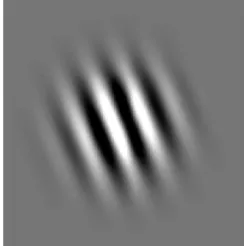
[image:28.612.245.369.340.463.2]This section describes the mathematics behind Gabor wavelets, their use in a constructing a jet, and their contribution towards face recognition. Gabor wavelets are biologically motivated convolution kernels and they exhibit desirable characteristics of spatial locality and orientation selectivity. As a result, the Gabor transformed face images produce salient local and discriminating features that are suitable for face recognition. The representation of local features in this work is based on the Gabor wavelet transform.
Figure 5. A 2D Gabor Wavelet.
The kernel of the Gabor wavelet consists of two components: the plane wave, with a constant frequency, orientation and amplitude, and a Gaussian envelope that restricts it. The generalized equation of a 2D Gabor wavelet kernel is given below.
𝜓𝜓𝜇𝜇,𝜈𝜈(𝑥𝑥⃗) =�𝑘𝑘�������⃗�𝜇𝜇,𝜈𝜈
2
𝜎𝜎2 𝑒𝑒−
�𝑘𝑘��������⃗�𝜇𝜇,𝜈𝜈 2‖𝑥𝑥⃗‖2
2𝜎𝜎2 �𝑒𝑒𝑖𝑖𝑘𝑘��������⃗𝑥𝑥⃗𝜇𝜇,𝜈𝜈 − 𝑒𝑒−𝜎𝜎
2
2� (2.8)
where 𝜇𝜇 and 𝜈𝜈 define the orientation and scale of the Gabor kernels, 𝑥𝑥⃗= (𝑥𝑥,𝑦𝑦), ‖.‖
𝑘𝑘𝜇𝜇,𝜈𝜈
�������⃗= �𝑘𝑘𝜈𝜈cos𝜑𝜑𝜇𝜇
𝑘𝑘𝜈𝜈sin𝜑𝜑𝜇𝜇�, 𝑘𝑘𝜈𝜈 = 2
−𝜈𝜈+22 𝜋𝜋, 𝜑𝜑
𝜇𝜇 = 𝜇𝜇𝜋𝜋8 (2.9)
A set of convolutions for kernels of different orientations and frequencies at one image pixel is called a jet. A jet describes a small patch of a grayscale image 𝐼𝐼(𝑥𝑥⃗′), around a given pixel 𝑥𝑥⃗= (𝑥𝑥,𝑦𝑦). It is based on the Gabor wavelet transform, which is defined as the following convolution.
𝐼𝐼(𝑥𝑥⃗)∗ 𝜓𝜓𝜇𝜇,𝜈𝜈(𝑥𝑥⃗) =∫ 𝐼𝐼(𝑥𝑥⃗′)𝜓𝜓𝜇𝜇,𝜈𝜈(𝑥𝑥⃗ − 𝑥𝑥⃗′)𝑑𝑑2𝑥𝑥⃗′ (2.10)
where * denotes convolution. The jet used in this work uses a set of Gabor wavelets, from Equation (2.8), that covers eight orientations, 𝜇𝜇 = 0, … 7 and 5 frequency scales,
𝜈𝜈 = 0, … 4. We use a coefficient index 𝑖𝑖= 𝜇𝜇+ 8𝜈𝜈 to index the 40 different coefficients in the jet, with 𝑖𝑖 = 0, … 39. This sampling evenly covers a band in frequency space. The coefficients 𝒥𝒥𝑖𝑖(𝑥𝑥⃗) of the jet 𝒥𝒥 are defined with respect to equation (2.10) as follows:
𝒥𝒥𝑖𝑖(𝑥𝑥⃗) =� 𝐼𝐼(𝑥𝑥⃗′)𝜓𝜓𝜇𝜇,𝜈𝜈(𝑥𝑥⃗ − 𝑥𝑥⃗′)𝑑𝑑2𝑥𝑥⃗′ (2.11)
The second term in the brackets of Equation (2.8) makes the Gabor wavelet kernels DC-free. Gabor wavelets are robust as a data representation because of their biological relevance. Since they are DC-free, they also provide robustness against varying brightness in the image. The limited localization in space and frequency provides some robustness against translation, distortion, rotation and scaling. Only the phase changes drastically with translation, but can safely be ignored.
compensated for its variation explicitly. The similarity function used in this work for comparing two jets, 𝒥𝒥 and 𝒥𝒥′, is
𝑆𝑆𝑎𝑎(𝒥𝒥,𝒥𝒥′) = ∑ 𝑎𝑎𝑖𝑖𝑎𝑎 ′
𝑖𝑖 𝑖𝑖
�∑ 𝑎𝑎𝑖𝑖 𝑖𝑖2∑ 𝑎𝑎𝑖𝑖 ′𝑖𝑖2 (2.12)
This function ignores phase, and has been used extensively in previous works [20]. With a jet 𝒥𝒥 taken from a fixed image position and jets 𝒥𝒥′ =𝒥𝒥′(𝑥𝑥⃗) taken at a variable position
𝑥𝑥⃗, 𝑆𝑆𝑎𝑎(𝒥𝒥,𝒥𝒥′(𝑥𝑥⃗)) is a smooth function with local optima. Equation (2.12) builds the basis
of using jets of Gabor wavelet-convoluted coefficients for recognition purposes, and is used in all other recognition concepts.
2.3. Elastic Bunch Graph Matching
This section covers details on Elastic Bunch Graph Matching, which is a recognition scheme that builds a face model using Gabor wavelet-based jets as a feature descriptor. The basic recognition scheme introduces in this section is considered as the base evaluation scheme for the procedures introduced in Chapters 4 and 5. The first sub-section describes how face models are represented, and the second sub-sub-section describes how the actual recognition process is carried out.
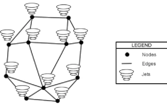
Figure 6. A Model Graph structure representing nodes and edges.
A model graph, as implemented by Wiskott et al [9], uses jets generated from Gabor-wavelet based convolution for the representation of local features at the nodes of the graph structure. Wiskott et al also incorporate distance information along the graph edges. When the labeled graph, along with its jet information, is stored into a library, it is called a model graph. When a new labeled graph is generated from a new image, it is called an image graph. Image graphs can be stored into the library to become model graphs, or be directly used for recognition against the existing model graph library.
Figure 7. A Bunch Graph stores jet bunches for each feature point and the average edge distances between them from all the faces.
2.3.1 Face Representation
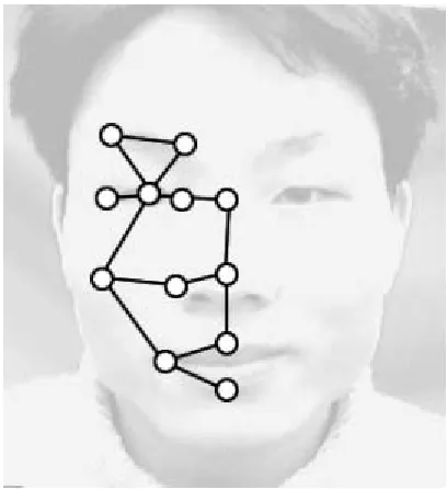
Figure 8. Fiducial points used from only one side of the face, connected by a face graph structure.
A labeled graph 𝒢𝒢 represents a face consisting of 𝑁𝑁 nodes on the fiducial points at positions 𝑥𝑥⃗𝑛𝑛,𝑛𝑛 = 1, … ,𝑁𝑁. The nodes are labeled with jets 𝒥𝒥𝑛𝑛. The edges are labeled with
distances ∆𝑥𝑥⃗𝑒𝑒 = 𝑥𝑥⃗𝑛𝑛 − 𝑥𝑥⃗𝑛𝑛′,𝑒𝑒 = 1, … ,𝐸𝐸, where edge 𝑒𝑒 connects node 𝑛𝑛′ with 𝑛𝑛. Hence the
edges are two-dimensional vectors. A labeled graph without the jet information is called a grid. The graph structure used in this work is maintained across pose variation, in terms of correspondence between feature points across pose. However, since there is significant variation in geometry and local features, bunch graphs are separately created for each different face pose trained.
best fitting jet from a bunch for each fiducial point. This is done so as to cover a much larger range of facial variation than represented in the trained models.
If, for a particular pose, there are 𝑀𝑀 model graphs 𝒢𝒢𝐵𝐵𝑚𝑚,𝑚𝑚 = 1, … ,𝑀𝑀, from which
a face bunch graph (FBG) is generated. The resultant face bunch graph would have the same structure, with its nodes linked with bunches of jets 𝒥𝒥𝑛𝑛,𝐵𝐵𝑚𝑚,𝑛𝑛 = 1, …𝑁𝑁, and its edges
linked with the average distances of the corresponding edges, ∆𝑥𝑥⃗𝑒𝑒𝐵𝐵 =𝑀𝑀1 ∑ ∆𝑥𝑥⃗𝑚𝑚 𝑒𝑒𝐵𝐵𝑚𝑚,𝑒𝑒 =
1, … ,𝐸𝐸.
2.3.1.1 Manual Definition of Graphs during Training
For initial training of the EBGM, the face grid is manually fit by selecting the individual positions of the node points by visual judgment for their best fit positions. Once the nodes in the grid are manually placed, the edges between the nodes are charted out, and the edge information is obtained from the difference of the node positions. Finally, the jets at the nodes are obtained from the image to create the model graph.
2.3.1.2 Automatic Fiducial Point Placement
This work implements only a portion of the entire automation algorithm proposed by Wiskott et al, which deals with positioning the individual nodes after the entire face grid is placed over the face. Due to the limitation of the Gabor wavelets, it is assumed that the node points are within an error of eight pixels from the manually preferred best-fit node positions prior to this procedure, so as to get best estimates. The necessary equations were developed by Wiskott et al [9] and are reproduced below for convenience.
The phase information available in the jets can be used as a means for jet localization in the image, since it varies so quickly with change in location. Assuming that two jets 𝓙𝓙 and 𝒥𝒥′ refer to object locations with a small displacement 𝑑𝑑⃗, the phase shift on the wave vector 𝑘𝑘�⃗𝜇𝜇,𝜈𝜈 can be approximated as 𝑑𝑑⃗𝑘𝑘�⃗𝜇𝜇,𝜈𝜈. Equation (2.12) for jet
similarity, can be made phase-sensitive, and re-written below.
𝑆𝑆𝜙𝜙(𝒥𝒥,𝒥𝒥′) =
∑ 𝑎𝑎𝑖𝑖 𝑖𝑖𝑎𝑎′𝑖𝑖cos(𝜙𝜙𝑖𝑖 − 𝜙𝜙′𝑖𝑖 − 𝑑𝑑⃗𝑘𝑘�⃗𝑖𝑖)
�∑ 𝑎𝑎𝑖𝑖2∑ 𝑎𝑎′𝑖𝑖2
𝑖𝑖 𝑖𝑖
(2.13)
The above equation reaches a maximum as the geometric distance between the two locations, which relate to the jets 𝒥𝒥 and 𝒥𝒥′, gets closer to zero. Thus, maximizing the equation (2.13), will give the displacement estimate 𝑑𝑑⃗. Maximizing the similarity function 𝑆𝑆𝜙𝜙(, ) is done in its Taylor expansion form:
𝑆𝑆𝜙𝜙(𝒥𝒥,𝒥𝒥′)≈∑ 𝑎𝑎𝑖𝑖𝑎𝑎 ′
𝑖𝑖[1−0.5(𝜙𝜙𝑖𝑖 − 𝜙𝜙𝑖𝑖′ − 𝑑𝑑⃗𝑘𝑘�⃗𝑖𝑖)2] 𝑖𝑖
�∑ 𝑎𝑎𝑖𝑖 𝑖𝑖2∑ 𝑎𝑎𝑖𝑖 ′𝑖𝑖2
(2.14)
Solving for 𝑑𝑑⃗ in the above equation gives the solution:
𝑑𝑑⃗(𝒥𝒥,𝒥𝒥′) =�𝑑𝑑𝑥𝑥
𝑑𝑑𝑦𝑦�=
1
Γ𝑥𝑥𝑥𝑥Γ𝑦𝑦𝑦𝑦 − Γ𝑥𝑥𝑦𝑦Γ𝑦𝑦𝑥𝑥 ×�
Γ𝑦𝑦𝑦𝑦 −Γ𝑦𝑦𝑥𝑥
−Γ𝑥𝑥𝑦𝑦 Γ𝑥𝑥𝑥𝑥 � �
Φ𝑥𝑥
Φ𝑦𝑦� (2.15)
Φ𝑥𝑥 = � 𝑎𝑎𝑖𝑖𝑎𝑎𝑖𝑖′𝑘𝑘𝑖𝑖𝑥𝑥 �𝜙𝜙𝑖𝑖 − 𝜙𝜙′𝑖𝑖� 𝑖𝑖
, Γ𝑥𝑥𝑦𝑦 = � 𝑎𝑎𝑖𝑖𝑎𝑎𝑖𝑖′𝑘𝑘𝑖𝑖𝑥𝑥𝑘𝑘𝑖𝑖𝑦𝑦 𝑖𝑖
and Φ𝑦𝑦,Γ𝑦𝑦𝑥𝑥,Γ𝑥𝑥𝑥𝑥,Γ𝑦𝑦𝑦𝑦 are defined accordingly. In all the above equations, the phase
difference has to be corrected to be within the range of ±𝜋𝜋. The distance estimate obtained in Equation (2.15) gives the best-guess displacement to the local best-fit location for the concerned node jet, which can be applied to the current node position as a correction.
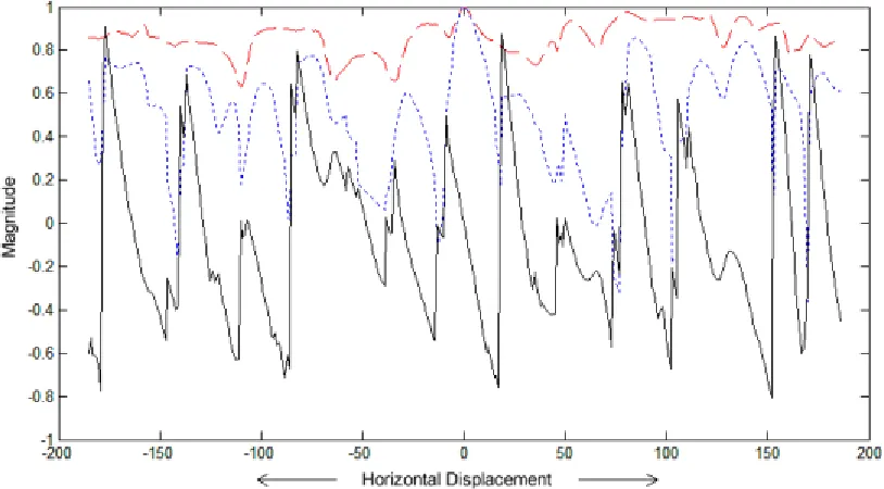
[image:36.612.105.512.376.601.2]The following graph plots out the displacement estimation for an arbitrary point in a sample face image along its horizontal. It can be inferred that the displacement estimation function is accurate within a few pixels of displacement from its expected best fit position. As seen from the graph, this is a ±6 pixel window around the best fit point.
Figure 9. Displacement Estimation: (a) Similarity without phase (shown in dashed line), (b) Similarity with phase (shown in dotted line), and (c) Displacement
2.3.2 Face Recognition
Recognition is carried out by use of the jet similarity functions. The similarity function, without phase, as represented in Equation (2.12) is used, since it would be more consistent across small variations, such as expression, etc., for the face of the same individual over different images. For recognition to be performed, model graphs of a set of faces have to be trained into the library, and an image graph from a query face image has to be obtained, either by manual placement or automatic placement procedure. The image graph is then compared against each model graph in the library, using a graph similarity function, and the comparison with the highest graph similarity is chosen as the matched pair.
There can be two distinct types of recognition that might need to be carried out. The first case is when both the model graph and image graph belong to the same face pose. This is the most direct approach, where all the jets have proper correspondence with their counterparts in either graphs. For an image graph 𝒢𝒢𝐼𝐼 and a model graph 𝒢𝒢𝑀𝑀, the
graph similarity function is defined as:
𝑆𝑆𝒢𝒢(𝒢𝒢𝐼𝐼,𝒢𝒢𝑀𝑀) =𝑁𝑁 � 𝑆𝑆1 𝑎𝑎(𝒥𝒥𝑛𝑛,𝐼𝐼,𝒥𝒥𝑛𝑛,𝑀𝑀) 𝑁𝑁
𝑛𝑛=1
(2.16)
where N is the total number of nodes in the graph. The second case of recognition is when recognition is being done across different graphs. In this case, the above function is modified so as to compute the average similarity of only the nodes that have correspondence between the two graphs. If 𝐾𝐾 nodes have correspondences between the graphs, and the node 𝑝𝑝𝑘𝑘 in the image graph corresponded to node 𝑞𝑞𝑘𝑘, 𝑘𝑘= 1, … ,𝐾𝐾, then
𝑆𝑆𝒢𝒢(𝒢𝒢𝐼𝐼,𝒢𝒢𝑀𝑀) =𝐾𝐾 � 𝑆𝑆1 𝑎𝑎(𝒥𝒥𝑝𝑝𝑘𝑘,𝐼𝐼,𝒥𝒥𝑞𝑞𝑘𝑘,𝑀𝑀) 𝑘𝑘
(2.17)
However, in this thesis, the graphs across the various trained poses have been confined to a very small set of fiducial points such that the graphs have corresponding indices for all the nodes, so Equation (2.16) will be used for all cases of face recognition.
Chapter 3
Automatic Feature Point Positioning
This chapter introduces a proposed feature point placement scheme that implements a combination of Active Shape Models and Elastic Bunch Graph Matching, which have been discussed in Chapter 2 as background information.
Multi-pose face recognition is a direct extension of frontal face recognition. However, recognition across pose, or pose-variant face recognition, uses a query image with a different face pose for which an image does not exist in the library. In either situation, there are two generalized approaches to face recognition: model-based and appearance-based. Model-based approaches try to build a 2D or 3D model of the face, with feature descriptors that represent different segments of the face model, and make use of this model during recognition. Appearance-based approaches use direct pixel information from the image to perform the recognition.
This thesis uses a model-based face recognition approach and it extracts face features that are crucial to the recognition performance. There are several automated algorithms that detect faces in an image frame. However, face detection alone is not sufficient for face recognition. It is also essential that the features selected for recognition align well with the face, so that the individual feature descriptors used for recognition provide the best match results against the feature descriptors present in the library.
Variation in face pose creates the following two problems for local face features: (a) Face features points can be obstructed in some face pose angles, preventing
matching of all features across poses.
The selection of feature points used for face recognition across pose variation should consider these cases, so that a good set of features are represented. Furthermore, locating these features in the image frame should be easy to automate, so that manual intervention can be avoided. This chapter describes the implementation for automatically selecting the best fit locations of the feature points used in face recognition, while the following chapters will describe the importance of these feature nodes with respect to the face recognition.
Section 3.1 describes a priori information that is required for the proposed automatic feature point placement scheme and reasons the need for it. Section 3.2 describes the actual procedure that is proposed in this chapter, while the final section in this chapter performs an evaluation of the proposed procedure.
3.1. Obtaining a priori Information
This thesis implements a combination of Active Shape Models (ASMs) and Elastic Bunch Graph Matching (EBGM) to track the positions of the features of interest on a face at any pre-trained pose. A good initialization of feature points is crucial to getting good placement results for any search algorithm. The effects of poor initialization for an ASM search algorithm can be
(i) prolonged convergence time, and/or (ii) convergence to non-face local matches.
For initializing the ASM search space by confining feature positions, this thesis work currently obtains the location information of the eyes and mouth manually through interactive input. However, these selected features (eyes and mouth) can be detected through a series of well-trained Harr-cascade filters [3]. This would be an inexpensive alternative for finding the eyes and mouth features automatically without manual feedback.
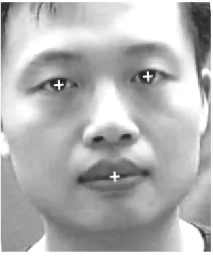
Another parameter that needs to be given as prior knowledge is the face pose angle. Face pose estimation is a separate area of research and is outside the scope of this work. This thesis assumes that the location information of these three facial features (left eye, right eye, and mouth) and the face pose parameter can be obtained from a priori
[image:41.612.232.383.374.557.2]steps dealing with pose estimation [21].
Figure 10. A Face Image with locations of features given as priori information.
3.2. Automatic Placement Scheme
Knowing the positions of a few key feature points in the image frame allows the estimation of the scale and orientation of the face in the image frame. However, the most important step for proper face recognition results would be the alignment of the face image with the face images in the library. Although Gabor-wavelet based jets can withstand small variations in image orientation, it is still important that this variation is removed, since this thesis work tries to measure recognition improvement along other parameters. Section 3.2.1 describes this procedure.
After the face image is aligned, the next step is to select an ASM that corresponds to the face pose parameter given as a priori information, and fit it along the feature points used for face alignment, extract the points necessary for face recognition, and use a combination of heuristics and jet-displacement estimations to best-fit the positions of these points over the fiducial points of the face. Section 3.2.2 describes this procedure.
Figure 11. Block Diagram illustrating Automatic Feature Point Positioning.
3.2.1 Correcting Face Image Alignment
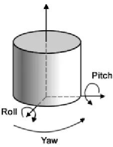
rotations are generally called yaw, pitch and roll, or can be collectively described as Euler angles.
Figure 12. Rotation components: Yaw, Pitch and Roll.
This thesis tries to study the impact on certain algorithms by variation of only one of these 3D rotation parameters – Yaw. For this, it is necessary to remove all other rotation parameters as much as possible. The simplest way to do this on a 2D face image would be to perform an affine transform that involves a 2D rotation, on the face image.
In order to perform the affine transform, the first step is to determine the center of face and the angle of rotation to be introduced. The angle of rotation 𝜃𝜃𝑟𝑟𝑟𝑟𝑡𝑡 is the angle
made by the line passing through the two eyes with the horizontal axis of the image frame. The face center is roughly estimated to be the point of intersection of the perpendicular from the mouth center to the line passing through the two eyes.
Figure 13. Face Alignment Process.
3.2.2 Find the best-fit locations of fiducial points
Figure 14. The Different ASM Shapes Used For Covering Pose Angle Variation. From the face pose parameter, which is a priori information, the appropriate ASM model is selected. Given the estimated feature points on the image after face alignment, it is possible to initialize the selected ASM model such that the scale, orientation and position of the model corresponds to the scale, orientation and position of an ASM to which the given estimated features belong. This process is exactly similar to the process used in model alignment while constructing the ASM model library in Section 2.1.2.
Once initialized, the ASM is made to run until it converges to the face shape in the image frame, or until an iteration count is reached. The next phase is to extract the node points in the ASM contour that will help align a face graph.
ensure the proper placement of the feature points, prior to extracting the feature information from the face image frame.
Figure 15. Example of fitting the ASM to extract the required graph node positions: (a) Fitting ASM on face image, (b) Selecting points from ASM that are needed, and (c)
Using extracted points to place face graph.
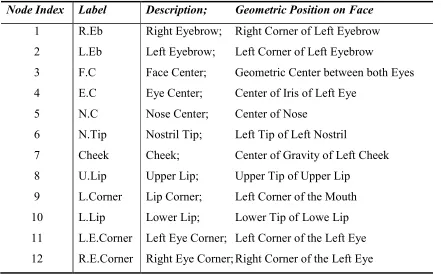
Table 1. Description of the Feature Points used in recognition.
Node Index Label Description; Geometric Position on Face
1 R.Eb Right Eyebrow; Right Corner of Left Eyebrow 2 L.Eb Left Eyebrow; Left Corner of Left Eyebrow
3 F.C Face Center; Geometric Center between both Eyes 4 E.C Eye Center; Center of Iris of Left Eye
5 N.C Nose Center; Center of Nose
6 N.Tip Nostril Tip; Left Tip of Left Nostril
7 Cheek Cheek; Center of Gravity of Left Cheek 8 U.Lip Upper Lip; Upper Tip of Upper Lip
9 L.Corner Lip Corner; Left Corner of the Mouth 10 L.Lip Lower Lip; Lower Tip of Lowe Lip 11 L.E.Corner Left Eye Corner; Left Corner of the Left Eye 12 R.E.Corner Right Eye Corner; Right Corner of the Left Eye
Figure 16 Face Graphs Used for Different Face Poses
[image:47.612.89.527.97.541.2]features, such as upper lip and nostril, jet displacement estimation is used to provide the best-guess positions. It is important to note that the initial node position extracted from the ASM model might not always be within a six pixel error limit of the preferred node position. When this initial position used in jet displacement calculation has an estimation error greater than a six pixels, the resultant displacement calculation will be erroneous. Hence, jet displacement estimation is used only for some nodes that have a good initial placement via the ASM models.
Figure 17. Example of finding best fit points around the eyes; (a) Initial Estimates, (b) Finding closest edges passing threshold, (c) Corrected Feature Points.
Figure 18. Example of finding Lip Corner By Finding the Steepest Edge in the neighborhood; (a) Initial Estimate, (b) Finding corner, (c) Corrected Feature Point.
The eye is typically a high-contrast region, with the contours of the eye being very distinctive. An edge map of the eye region would clearly indicate the periphery of the eyes. Furthermore, the structure of the eye is such that it tapers towards the side extremities. Hence, searching for the left and right extremities of the edge-map of the eye would directly provide the best-fit locations for the corner points of the eyes, as marked in Figure 17.
The lip corner is another feature point that can be located in a similar manner, since it is a high-contrast point and has a very low grayscale codevalue in its image neighborhood. Using the initial estimates from the ASM model as a proximity to the possible best-fit region, a search can be performed to find the high-contrast edge-map in the locality. The search finds the left tip of the edge-map, and confirms that it is the darkest point in its locality. This point is assumed to be the best-fit point for the lip corner, as indicated in Figure 18.
The heuristic searches explained above have been quite accurate in marking the feature points, when tested over a broad range of faces, and have thus been accepted as a usable heuristics for the mentioned feature points. The next section evaluates the performance of the automatic feature point placement scheme that has been introduced in this chapter.
3.3. Evaluation of the procedure
It is expected that the performance of the automatic feature selection scheme introduced in this chapter will perform worse than manual feature selection. However, the degradation is not expected to be large enough to negate the improvement in recognition by the steps introduced in this thesis work, as compared to the initial recognition procedures.
Figure 19. Example of Automatic Feature Point Positioning in Comparison with Manually Selected Nodes.
In order to be able to estimate the effects of automatic feature point placement for different recognition schemes, the evaluation of all the schemes is performed for both automatic as well as manual placement procedures. The graph in Figure 20 illustrates the effect of automatic feature point placement compared to manual feature point placement for the Direct Recognition scheme. Similar evaluations will be done for all the other schemes.
angles. This is because the features are better defined in these smaller poses. As the face pose increases, the distortion in the features become much more prominent in comparison to the frontal faces as well as other faces in the same pose.
Figure 20. Recognition rates for Direct Recognition scheme.
This chapter has described a proposed method for automatically positioning the facial feature points, which is used in automating the face recognition schemes described in the upcoming chapters. Chapter 4 introduces some of the preliminary methods proposed by this thesis. Chapter 5 introduces a proposed recognition scheme that shows promising results for large face pose variation, and also modifies it using some of the methods introduced in Chapter 4.
40% 50% 60% 70% 80% 90% 100%
15° 30° 45°
Rec
og
ni
ti
on
Ra
te
Face Pose Angle
Recognition Rates of Implemented Algorithms
Chapter 4
Feature Weighting and Face Derotation
The previous chapter introduced a procedure for automatically placing feature points required for face recognition. This procedure is utilized in the two different recognition schemes introduced in this chapter, each of which takes on a different approach to improving the recognition rates with variation in face pose. Section 4.1 reviews the basic recognition scheme that has been used in Elastic Bunch Graph Matching, which has been briefly covered in Chapter 2 as background information. This is pertinent to the recognition schemes proposed in this chapter. Section 4.2 introduces a scheme that makes up for some of the shortcomings of the basic recognition scheme. Section 4.3 introduces a completely different approach to trying to improve the face recognition across face pose.
Gabor wavelets are a common tool used in recognition schemes. The convolution of Gabor wavelets of different scales and orientations over a point in an image results in a set of complex coefficients which is called a ‘jet.’ A ‘jet’ is a representation of information contained in the neighborhood of the image point where the jet was constructed. This thesis uses a set of Gabor wavelets spanning five frequency scales and eight orientations, totaling to forty individual convolution results. Hence, any one jet will contain forty complex coefficients.
Figure 21. Direct Recognition Scheme.
4.1. Face Recognition Using Elastic Bunch Graph Matching
Elastic Bunch Graph Matching represents faces as face graphs, with nodes linked with jets used as feature descriptors. The similarity function 𝑆𝑆𝑎𝑎, introduced in Section 2.2 of
Chapter 2, for comparing two jets corresponding to points only a few pixels apart, tries to compare the closeness of each pair of coefficients from two jets 𝒥𝒥 and 𝒥𝒥′, and computes a
similarity value. This similarity value of two jets can be as low as zero, if there is no correlation at all between the coefficients of the jets. Equation (2.12) representing the similarity function is repeated here for convenience:
𝑆𝑆𝑎𝑎(𝒥𝒥,𝒥𝒥′) = ∑ 𝑎𝑎𝑖𝑖𝑎𝑎 ′
𝑖𝑖 𝑖𝑖
�∑ 𝑎𝑎𝑖𝑖2∑ 𝑎𝑎′𝑖𝑖2
𝑖𝑖
𝑖𝑖 (4.1)
where 𝑎𝑎𝑖𝑖,𝑎𝑎𝑖𝑖′ are the corresponding coefficients of jets 𝒥𝒥 and 𝒥𝒥′, and 𝑖𝑖 = 1, … 39 is the
coefficient index in the jets. Equation (4.1) can be used to compare node-wise similarity between any two nodes in any two graphs. When comparing feature similarity, Equation (4.1) is used for finding the similarity between corresponding feature nodes of any two graphs.
match that has the highest similarity score [9]. The equation for computing the similarity of two graphs, each having 𝑁𝑁 corresponding nodes, is
𝑆𝑆𝒢𝒢(𝒢𝒢𝐼𝐼,𝒢𝒢𝑀𝑀) =𝑁𝑁 � 𝑆𝑆1 𝑎𝑎(𝒥𝒥𝑛𝑛,𝐼𝐼,𝒥𝒥𝑛𝑛,𝑀𝑀) 𝑛𝑛
,
where each node contributes an equal amount towards the whole face similarity value. If there are 𝐾𝐾 face graphs trained in the face library and a query is made, then an iterative comparison is performed between each of the K face graphs in the library and the face graph extracted from the query face image frame. The library face graph that has the highest similarity match value, against the query image face graph, corresponds to the best match. This is the basic recognition scheme used in Elastic Bunch Graph Matching [9]. This scheme is labeled as ‘Direct’ Recognition scheme in the comparison tests.
4.2. Feature Weighting Scheme
Section 4.1 reviewed the basic recognition scheme used in Elastic Bunch Graph Matching. As noted in the review, there is no discrimination on the facial features based on their ability to differentiate between faces. This section introduces a Feature Weighted Recognition Scheme, which studies the discrimination capability of the feature points used in face recognition and accordingly assigns a weight to each feature that affects the individual contribution of each feature towards the whole face recognition result.
4.2.1 Motivation
some features on the face are more distinguishing than others. For frontal face recognition, it is understandable that features such as the eyebrows, or eyes and mouth are much more distinguishing than other regions of the face. However, for recognition of faces across pose variation, another factor that plays an important role in considering the distinguishing features is the amount of deformation the features undergo over pose variation. Features that vary dramatically with variation in pose might not be suitable for identifying/distinguishing individuals in a group. Hence, a possible consideration is to give more importance to features that can discriminate faces properly at a particular face pose. Effectively, a different set of weights can be used while calculating the total face similarity for different face poses.
4.2.2 Procedure
As previously mentioned, the Direct Recognition scheme selects the face match that has the highest similarity value during comparison. This scheme does not consider the individual contributions of each node in the graph. The following figures show the individual node similarity values of a correct face match at different face poses for one individual in the library.
Figure 22. Face Similarity of a sample face query image against the frontal face model in the library, with query face image at 15°, 30°, and 45° poses.
[image:56.612.99.514.79.339.2]However, some nodes have very distinct difference in similarity between the correct matches and incorrect matches. Giving more importance to these nodes might result in better recognition rates. Hence, it might be advantageous to numerically weigh the nodes according to their importance.
Figure 23. Weighted Recognition Scheme.
For convenience of representation, let 𝑆𝑆𝑖𝑖𝑛𝑛,𝑖𝑖 be the notational equivalent for the
similarity of the jets corresponding to the 𝑛𝑛th node of two face graphs, labeled 𝑖𝑖 and 𝑖𝑖.
where 𝑆𝑆𝑎𝑎�𝒥𝒥𝑛𝑛,𝑖𝑖,𝒥𝒥𝑛𝑛,𝑖𝑖� is the similarity function between two given jets, defined in
Equation (4.1).
In the notation used in Equation (4.2), it can be interpreted that if the face graph labels 𝑖𝑖 and 𝑖𝑖 point to one individual’s library and query face graphs, then Equation (4.2) is simply computing the similarity match value of the ‘correct match’. In a similar manner, if the labels 𝑖𝑖 and 𝑖𝑖 do not point to different face graphs of the same individual, the computed value can be considered as a similarity match value of an ‘incorrect match’. The notation 𝑆𝑆𝑖𝑖𝑛𝑛,𝑖𝑖 used in Equation (4.2) is for similarity between two jets or
features. Let this notation be extended to entire face graphs by following the notation 𝑆𝑆𝑖𝑖,𝑖𝑖,
where an absence of index 𝑛𝑛 indicates that whole graph is represented.
Comparing a query face with each face in a library set of 𝐾𝐾 faces will result in one correct match and 𝐾𝐾 −1 incorrect matches. Each of these matches will have a face graph similarity value 𝑆𝑆𝑘𝑘,𝑄𝑄, where the label 𝑘𝑘 points to the 𝑘𝑘th face in the library set, and
label 𝑄𝑄 point to the query face graph. Preferably, the face corresponding to the highest value of 𝑆𝑆𝑘𝑘,𝑄𝑄 would be the correct match. However, the highest similarity match value
may not always correspond to the correct match. It would be possible to get a more preferable result, if the nodes making a larger contribution to the difference in similarity with incorrect matches are given a larger weighting.
both the face indices are the same and an incorrect match is for any other index pair. Then the variance
𝜎𝜎𝑛𝑛2,𝑐𝑐𝑟𝑟𝑟𝑟𝑟𝑟𝑒𝑒𝑐𝑐𝑡𝑡 =𝜎𝜎2��𝑆𝑆𝑞𝑞𝑛𝑛,𝑞𝑞:𝑞𝑞= 1, …𝐾𝐾�� (4.3)
represent the variance in similarity of the 𝑛𝑛th node for a correct match, and
𝜎𝜎𝑛𝑛2,𝑖𝑖𝑛𝑛𝑐𝑐𝑟𝑟𝑟𝑟𝑟𝑟𝑒𝑒𝑐𝑐𝑡𝑡 = 𝜎𝜎2��𝑆𝑆
𝑝𝑝𝑛𝑛,𝑞𝑞 ∶ 𝑝𝑝 ≠ 𝑞𝑞; 𝑝𝑝,𝑞𝑞 ∈ (1, …𝐾𝐾)�� (4.4)
is the variance in similarity of the 𝑛𝑛th node for incorrect matches. be vector
The variance of correctly matched nodes indicates how reliable the nodes are in distinguishing features correctly, and the variance in incorrectly matched nodes indicates how unreliable the nodes are in discarding wrong matches. Hence a suitable set of weights would take the two variances into account. Fischer’s criterion can be applied in this context to calculate the weights using the two variances. Then, the weight for the 𝑛𝑛th
node would be
𝑊𝑊𝑛𝑛 = 𝜎𝜎𝑛𝑛,𝑐𝑐𝑟𝑟𝑟𝑟𝑟𝑟𝑒𝑒𝑐𝑐𝑡𝑡
2
𝜎𝜎𝑛𝑛2,𝑖𝑖𝑛𝑛𝑐𝑐𝑟𝑟𝑟𝑟𝑟𝑟𝑒𝑒𝑐𝑐𝑡𝑡 . (4.5)
The following graph plots the weights used in this work, for each of the nodes for the face graph structure implemented in face recognition. The weights {𝑊𝑊𝑛𝑛} have been
normalized to get {𝑊𝑊𝑛𝑛′} such that they total to a value of 1. This is just to avoid scaling up
the similarity value.
𝑊𝑊𝑛𝑛′ =�
𝑊𝑊𝑛𝑛 −min𝑛𝑛 (𝑊𝑊𝑛𝑛)
max𝑛𝑛 (𝑊𝑊𝑛𝑛)−min𝑛𝑛 (𝑊𝑊𝑛𝑛)� �
9
10�+ 0.1 (4.6)
feature point in the face graph used for the face recognition step. Figure 24 graphically represents the weights in Table 2.
Figure 24. Feature weights calculated for different pose graphs.
In Figure 24 and Table 2, the weights have been scaled down such that the sum of the weights of all features is equal to a value of 1.0, so as to avoid having the similarity value of the whole face multiplied by a scaling factor.
It can be noted that different features carry varying weights as the face pose changes. It is further notable from the table that certain features, such as the eye center, have a more distinguishable characteristic than others.
0 0.02 0.04 0.06 0.08 0.1 0.12 0.14
W
ei
gh
ta
ge
Node Lables
Normalized Weights
Table 2. Calculation of weights for 15°, 30° and 45° Face Pose Graph for a Sample Run using Equation (4.6).
Node #
(n) Lable
Calculated Weights, 𝑊𝑊𝑛𝑛𝑁𝑁
15° Pose 30° Pose 45° Pose
1 R.Eb 0.098 0.118 0.090 2 L.Eb 0.023 0.013 0.093 3 F.C 0.075 0.072 0.065 4 E.C 0.102 0.090 0.090 5 N.C 0.045 0.054 0.050 6 N.Tip 0.055 0.064 0.082 7 Cheek 0.031 0.021 0.085 8 U.Lip 0.107 0.112 0.095 9 L.Corner 0.115 0.125 0.100 10 L.Lip 0.099 0.095 0.013 11 L.E.Corner 0.125 0.121 0.106 12 R.E.Corner 0.124 0.114 0.125
From Figure 24, it can be deduced that some features have relatively lower generated weights at certain face pose angles than at other face pose angles. The lower lip (L.Lip) feature descriptor loses its significance for 45° face pose. This is primarily because the feature point lies along the face contour at a 45° face pose, while it is significantly distant from the periphery at smaller pose angles. This creates a tremendous difference in neighborhood information between the larger and smaller face poses, and hence almost incapacitates the feature from being able to perform recognition. As a result, lower weighting is given to that feature.
distorted as much as the other features, and hence have higher generated weights than those other features.
To implement the weights calculated in this section, the equation for computing the similarity of two graphs, each having 𝑁𝑁 corresponding nodes, has to be modified as:
𝑆𝑆𝒢𝒢(𝒢𝒢𝐼𝐼,𝒢𝒢𝑀𝑀) =𝑁𝑁 � 𝑊𝑊′1 𝑛𝑛 ∙ 𝑆𝑆𝑎𝑎(𝒥𝒥𝑛𝑛,𝐼𝐼,𝒥𝒥𝑛𝑛,𝑀𝑀) 𝑁𝑁
𝑛𝑛=1
(4.7)
It is to be noted that training is required to generate the weights suitable for a set of faces, as the weights might be different for different classes of faces. Also, the weights might vary with respect to the pose variation, as different facial features will not have the same similarity contribution as the face pose varies. Hence, the generation of these weights will require training prior to use in the recognition scheme.
This subsection described the procedure for implementing a proposed weighted recognition scheme, where features with better discriminating ability than others have been given higher weighting. The next subsection looks into evaluating the results obtained from the proposed scheme and makes interpretation on the utility of the proposed scheme.
4.2.3 Evaluation of Weighted Recognition Scheme
Since training is involved, it may not be ideal to use only a selective set of faces, as it might not always be the representative of a test set. Hence, a k-fold cross-validation approach is adopted, with the database divided into five discrete subsets. The k-fold cross-validation uses one subset for testing, and the remaining for the required training. Thus, 80 face pairs are used for training, and 20 face pairs used for testing.
Training involves calculating the feature weights as described in the previous section. Testing is done by taking a non-frontal face from the test set and running a similarity match against all the frontal faces in the test set to find a match. If the match is a correct match, it is considered as a hit, and if it is an incorrect match, it is a miss. Recognition rate is calculated as the percentage of hits in the total test set.
The evaluation of the Weighted Recognition scheme is done by determining the change in the recognition hit rate for the Direct Recognition scheme as well as the Weighted Recognition scheme over the same test set of faces. This is done using both manual and automatic feature point placement, as explained in Chapter 3.
Table 3. Evaluation Results for Weighted Face Recognition scheme using Manually Positioned Feature Points for 15° Face Pose Query Images.
Run Number # of Test Faces # of Training Faces Face Recognition Direct
# (%) Weighted # (%) Impr