Mathematical Models of the Infinite Porous Rotating Disk Electrode

Int. J. Electrochem. Sci., 13 (2018) 9999 – 10022, doi: 10.20964/2018.10.35

International Journal of

ELECTROCHEMICAL

SCIENCE

Mathematical Models of the Infinite Porous Rotating Disk

Electrode

J. Visuvasam1, A. Molina2, E. Laborda2, L. Rajendran1,*

1 _{Academy of Maritime Education and Training(AMET), Deemed to be University, Department of} Mathematics, Kanathur- 603112, India

2 _{Department of Physical Chemistry, University of Murcia, 30100 Murcia, Spain.} *_{E-mail: [email protected]}

Received: 27 April 2018 / Accepted: 29 May 2018 / Published: 1 September 2018

An analytical expression of the current generated from the electrochemical reaction in a porous rotating disk electrode (PRDE) is derived when the reactant transport is dominated by advection and diffusion. Simple algebraic expressions for the concentration of reactant and the current response are obtained as a function of the rotation rate, reaction rate, permeability of the porous medium, diffusion coefficients, kinematic viscosity, and geometry of the porous film. Upon comparison, the analytical expression of current in this work coincides with the existing results for the limiting case of low rotation rates. Also the concentration/current expressions here derived are in satisfactory agreement with numerical results.

Keywords: Mathematical modelling, Porous rotating disk electrode, Non-linear convection diffusion equation, Homotopy perturbation method.

1. INTRODUCTION

to an expression for the desired solution in terms of a formal power series in some "small" parameter – known as a perturbation series – that quantifies the deviation from the exactly solvable problem. Generally, the perturbation method is valid only for weakly non-linear problems. The combination of the perturbation and the homotopy methods eliminates the above drawbacks of the traditional perturbation method while keeping all the advantages.

In the present work, the HPM method is used to treat the problem of the uniformly-accessible porous rotating disc electrode (PRDE) under steady state conditions. The use of porous materials as electrodes are found in many electrochemical technologies and devices, including batteries [14,15], fuel cells [16] and capacitors[17], in electrolytic cells [18] as well as in electro analytical sensors [19-22]. In general, these systems allow for larger current densities than uniform flat electrodes, with benefits in terms of power output, electrolysis yield or sensitivity. The mass transport in the film, as a function of the porous morphology, and the electrochemical kinetics mostly determine the electrolysis efficiency. The mathematical modelling of these processes in the case of stationary porous electrodes was developed in the last decade[19,23,24]. In contrast, theoretical studies of hydrodynamic methods, such as the PRDE, which can be employed in the evaluation of materials electrocatalytic activity, are much more limited[25,27]likely due to the higher complexity of the advection-diffusion problem. Thus, the flow in a porous disc electrode was discussed by Joseph [27] for an infinite permeable disc steadily rotating in an unbounded fluid. Blaedel and Joseph [28] presented the electrochemical characterization and the analytical use of porous carbon rotating disc electrodes. More recently, Nam et al. [25] obtained expressions for the steady-state concentration of the reactant and the PRDE current using the conventional perturbation technique.

In this work, analytical expressions will be deduced for the concentration profile of the reactant and for the overall rate of transformation (the current generated) as a function of the reaction kinetics, the film permeability (k) and thickness, and the rotation rate, among other parameters. The closed-form solutions presented can assist the optimization of electrochemical devices and operating conditions, as well as the evaluation of the electrocatalytic activity of the film material.

2. MATHEMATICAL FORMULATION OF THE PROBLEM

The dimensionless form of the convection-diffusion transport problem of the reactant close to the PRDE surface can be expressed as follows after eliminating all radial dependence assuming that the depletion/boundary layer is very thin compared to the radius of the film [25]:

2 2 f 2

dz c d v D dz dc ) Z

(   (1)

cˆ k dz

cˆ d v D dz

cˆ d ) Z

( r

2 2 p

 

   

 (2)

  1, z

c ₍₃₎

  0, z

cˆ (4)

0 z , cˆ

c  ₍₅₎ 0

z , dz

cˆ d D D

dz dc

f

p _



(6) Using the following dimensionless variables

1/3 f

1/6 9

2 5 2 4

f

p

f

1/3

2 2 f

1/3

r r

2 f

3

3 9

B 2

D

3 9

G 2

3 9

K

z y

D

k h

D

D

D

k

D

k k

D

 

 

  _{ } 

 

 

 

  _{ }

 _  _



 



  _{ }

 _  _

  

  _{ }

    _{ }

(7)

equations (1)-(6) become in dimensionless form as follows:

2 2 2

dy c d dy dc ) B y 3

(  

 (8)

cˆ K dy

cˆ d D dy

cˆ d ) B Gy (

2 2

 



 (9)

Assuming that (i) the concentration of reactant in the fluid far from the interface is its bulk concentration, (ii) at deep inside the porous disk, the concentration of reactant in porous media is zero (since the reactant is completely consumed in the boundary layer), (iii) the concentrations and flux of reactant in the fluid and porous media are equal at the fluid-porous disk boundary(y=0), the boundary conditions are defined as follows:

  1, y

c (10)

  0, y

cˆ (11)

0 ,

ˆ 

c y

c (12)

0 y at , dy

cˆ d D dy

dc_{ }

(13) From the concentration profile of the reactant inside the porous film where the first-order redox reaction takes place, the current response can be calculated as





V

rc n F dV k

I ˆ (14)

       

 1/2 _0_ M

R cˆ dy

h V

I I

I 

 (15)

where the maximum currentIMis defined as [25]

2 M r

I  k c n F R h_

(16) 3. ANALYTICALRESOLUTION OF THE PRDE PROBLEM USING THE HOMOTOPY PERTURBATION METHOD (HPM)

By solving equations (8) and (9) using the homotopy perturbation method (Appendix A), the following expressions for the concentration of the reactant in the fluid phase and porous media are obtained:                   3 1 3 2 1 , 3 2 , 3 1 ) ( 1 )

(y m k y Bm y

c (17)

    _{  }  2 1 0 1 4 ) ( ˆ y a b y l l k e y

c ay (18)

where,





1 1

1 1 2

2 1

0 1 1 2 2 1

3

, , , ,

3 3 2.6789 3 2.6789

3 2.6789

, , , 1.3541 ,

2.6789 3 4 2

o

D l l a l l

D k a Gk a

m k k b

D a D

l D l B b m K

l m k a l l B m a

D a D a a D

                      (19)

These results (Eqns. (17) and (18)) can be re-written in terms of the important dimensionless quantities B, G, D and K as follows:

                                                    3 0 3 0 0 , 3 2 , 3 1 505468 . 0 2 3 4 3 6789 . 2 0623 . 4 373283 . 0 1 1 ) ( y b KD B y KD B D B KD G D KD B b KD b y c (20)                                    2 0 0 / 4 3 2 3 4 3 2 3 4 3 6789 . 2 0623 . 4 1 3 ) ( ˆ y D G y D B KD G D B KD G D KD B b b e y c y D K (21) where KD

b₀  32.6789 (22)

Using Eqns. (15) and (18), the following expressions are obtained for the current

                                         4 2 1 0 1 2 / 1 4 2 1 0 1 2 / 1 2 2 a b a l a l k h v I I a b a l a l k h v I I I R M R   (23)

The above equation can be re-written in terms of the dimensionless parameters B, G, D, and K:





1 0 8930 0 4514 0 8930 0 8930 0 75 0 5

1 0 8930

G D G B

. KD . B KD . . B . .

K KD K KD

I

D _{. KD}

     



The non-linear system of convection-diffusion equations (Eqs. (8) and (9)) with the corresponding boundary conditions (Eqs.(10–13)) has also been solved numerically via a finite-difference numerical method finding a reasonable agreement (less than 10 % error) for typical conditions ( 4

G10 0.1[12]) when K > 50 for B0 1. and K > 1000 for B1.

4. PREVIOUS ANALYTICAL EXPRESSIONS

Nam et al. [25] developed a mathematical model for an infinite porous disk electrode with G=0 and small values of B, obtaining the following expressions for the concentration profile of the reactant inside and outside the porous medium:





3 3 3

2 0

1

1 1 2

1

y

y y y

y y

KD e dy B KD y e dy KD b / e dy

c( y )

KDb

 

    

 _  _{ }   _{ }

 



 (25)

1 2

2 1

1

1 1

2 2 2

1

/

( K / D ) y y y

e B KD b KD b

D D

ˆc( y )

KD b

    

 _{   } 

    

 

  

 



 (26)

where

3 1

0

3 2

0

2 3

0 8930

9 2 3

0 4514

b exp( y ) dy .

( / ) b y exp( y ) dy .







   



  





(27)

Note that Eqns. (25) and (26) derived by Nam et al. [25] do not satisfy the boundary condition

0

 cˆ at y

c .

Using Eqns. (26) and (15), the current becomes,

1/ 2

1 1

R 1/ 2 1/ 2 2

1 1

2 1/ 2

b b

v h _ˆ 1 1

I I AD B b

(KD) 2 (KD) 2 (KD) 2

b b

D 1

ˆA 1 B KD b

K 2 2 (KD) 2

 _{  }

 

 

  _{  }       

   

 

    

      _  _

   

 

 

 

  

    

  

    

  

   



 _

 

 

2 b b KD KD

2 1 2

b B 1 Aˆ D K

I ₂ 1

2 / 1

1 ₍₂₈₎

where

1

1 1 ˆA

KD b



 1 0.8930 KD 1



5. LIMITING CASES

1. Limiting Case

The parameters B and G are directly proportional to the rotation rate. When diffusion dominates or there is no convection within the porous medium, then G = 0 and B = 0 and equations (8) and (9) become into:

0 dy dc y 3 dy c d ₂ 2 2 

 (30)

0 cˆ K dy cˆ d D 2 2   (31)

The exact solution of the above equation is given by:

) , 3 / 1 ( 6789 . 2 3 1 )

( y3

KD KD y c   

 ₍₃₂₎

KD e y c y D K 6789 . 2 3 3 ) ( ˆ 

 ₍₃₃₎

which are identical to Eqns. (20) and (21) after making G0 and B 0 (i.e.k₂     b m l₀ l₁ l₂ 0).

The current for G _{= 0 and B = 0 is given by,}

K D D K 8930 . 0 1 1 dy cˆ h v I I 0 2 / 1 R                   _      (34)

which coincides with Eqn. (24), and also with the result derived by Nam et al. [25] (Eqn. (28)) for B 0 . Moreover, when the reaction is very fast (K 1), Eqn. (34) reproduces the Levich equation for flat rotating disk electrodes since the reactant is consumed exhaustively on the surface of the disk [25]: 2 / 1 3 / 2 2 / 1 6 / 1 0867 . 0 p f D D D K

I  

 (35)

2. Limiting case

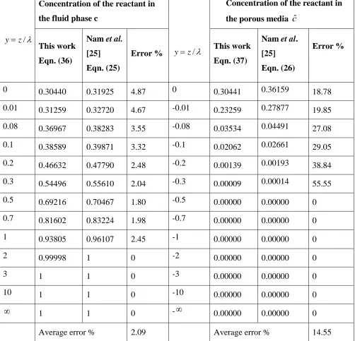
Table 1. Comparison of the analytical expression for the concentration of reactant in the fluid phase c and the porous mediacˆ with previous results. The numerical values of parameters are

, 0 ,

1 . 0 , 75 ,

1 .

0   

 K D and G

B



/

z y

Concentration of the reactant in the fluid phase c



/

z y

Concentration of the reactant in the porous media cˆ

This work Eqn. (36)

Nam et al.

[25] Eqn. (25)

Error % This work

Eqn. (37)

Nam et al. [25] Eqn. (26)

Error %

0 _{0.30440 0.31925 4.87} 0 _0.30441 0.36159 _18.78

0.01 _{0.31259 0.32720 4.67} -0.01 _0.23259 0.27877 _19.85

0.08 _{0.36967 0.38283 3.55} -0.08 _0.03534 0.04491 _27.08

0.1 _{0.38589 0.39871 3.32} -0.1 _0.02062 0.02661 _29.05

0.2 _{0.46632 0.47790 2.48} -0.2 _0.00139 0.00193 _38.84

0.3 _{0.54496 0.55610 2.04} -0.3 _0.00009 0.00014 _55.55

0.5 _{0.69216 0.70467 1.80} -0.5 _{0.00000 0.00000 0}

0.7 _{0.81602 0.83224 1.98} -0.7 _{0.00000 0.00000 0}

1 _{0.93805 0.96107 2.45} -1 _{0.00000 0.00000 0}

2 _{0.99998 1 0} -2 _{0.00000 0.00000 0}

3 _{1 1 0} -3 _{0.00000 0.00000 0}

10 _{1 1 0} -10 _{0.00000 0.00000 0}





Average error % 2.09 Average error % 14.55

1 2

1 0 1 2

2

1 0 8930 0 4514 0 8930

2

1 0 8930

/ R

k l l

v h

I I

a a

K B

. D . B KD . B

D KD

K K

. D

D D





 

 

 _{ } _  _

 

   

   



 



 

 

2

D K D 8930 . 0 1

KD 2

B B 8930 . 0 KD B 4514 . 0 D K D 8930 . 0 1

D K I

    

  



 

 

 (38)

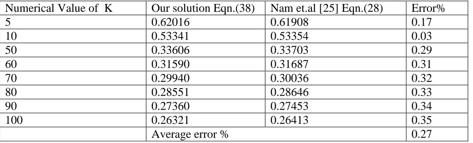
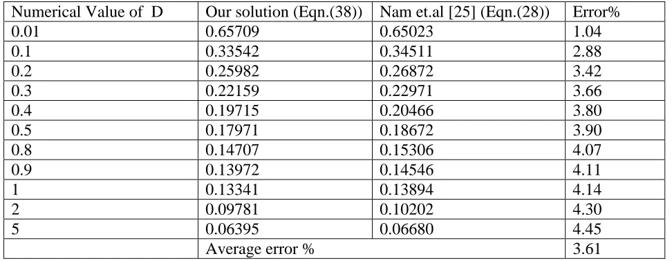
Equation (38) is compared with Eqn. (28) for various values of the parameters B, K, and D in Table (2A) - (2D) and reasonable agreement is found (differences smaller than 7%).

Table 2A. Comparison of the expression for the current (Eqn. (38)) with previous solution for G=0 (Eqn. (28)) for various values of K when D=0.1, and B=0.01.

Numerical Value of K Our solution Eqn.(38) Nam et.al [25] Eqn.(28) Error%

5 0.62016 0.61908 0.17

10 0.53341 0.53354 0.03

50 0.33606 0.33703 0.29

60 0.31590 0.31687 0.31

70 0.29940 0.30036 0.32

80 0.28551 0.28646 0.33

90 0.27360 0.27453 0.34

100 0.26321 0.26413 0.35

Average error % 0.27

Table 2B. Comparison of the expression for the current (Eqn.(38))with a previous solution for G=0 (Eqn.(28)) for various values of K when D=0.1, and B=0.1.

Numerical Value of K Our solution Eqn.(38) Nam et.al [25] Eqn.(28) Error%

5 0.68506 0.67425 1.58

10 0.57973 0.58109 0.23

50 0.35736 0.36706 2.71

60 0.33542 0.34511 2.89

70 0.31751 0.32712 3.03

80 0.30250 0.31199 3.14

90 0.28965 0.29899 3.22

100 0.27846 0.28766 3.30

Table 2C. Comparison of the expression for the current (Eqn. (38)) with a previous solution for G=0 (Eqn. (28)) for various values of D when K=60, and B=0.1.

Numerical Value of D Our solution (Eqn.(38)) Nam et.al [25] (Eqn.(28)) Error%

0.01 0.65709 0.65023 1.04

0.1 0.33542 0.34511 2.88

0.2 0.25982 0.26872 3.42

0.3 0.22159 0.22971 3.66

0.4 0.19715 0.20466 3.80

0.5 0.17971 0.18672 3.90

0.8 0.14707 0.15306 4.07

0.9 0.13972 0.14546 4.11

1 0.13341 0.13894 4.14

2 0.09781 0.10202 4.30

5 0.06395 0.06680 4.45

Average error % 3.61

Table 2D. Comparison of the expression for the current (Eqn. (38)) with a previous solution for G=0 (Eqn. (28)) for various values of B when K=60, and D=0.1.

Numerical Value of B Our solution (Eqn.(38)) Nam et.al [25] (Eqn.(28)) Error%

0.001 0.31395 0.31405 0.03

0.01 0.31590 0.31687 0.30

0.03 0.32024 0.32315 0.90

0.05 0.32458 0.32942 1.49

0.07 0.32891 0.33570 2.06

0.09 0.33325 0.34197 2.61

0.1 0.33542 0.34511 2.88

0.2 0.35710 0.37648 5.42

0.3 0.37878 0.40786 7.67

0.5 0.42215 0.47060 11.47

0.7 0.46551 0.53335 14.57

0.8 0.48720 0.56472 15.91

0.9 0.50888 0.59610 17.13

1 0.53056 0.62747 18.26

Average error % 7.19

From Tables (2A) – (2D), it is inferred that the error of Eqn. (28) decreases as B is smaller. Equation (28) is valid for small values of B whereas the present solution (Eqn.38) is valid for any B-value.

6. DISCUSSION

porous media G. The parameters B and G (convection term) are directly proportional to the rotation rate whereas the parameter K is inversely proportional to it. When the rotation rate is large, the transport of fluid to and through the porous disc is dominated by advection. However, when the rotation rate is small, diffusion becomes significant and in some cases it is the dominant mass transport mechanism.

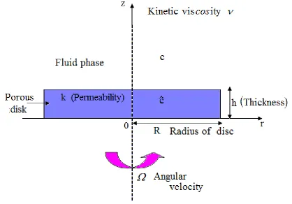
Figure 1. Schematic of a porous rotating disk electrode.

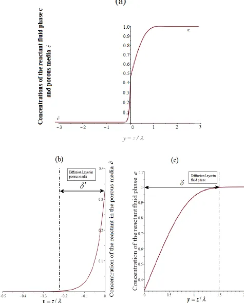
Figs.2-6 show the reactant concentration in the fluid phase c and in the porous media cˆ using Eqns.(20) and (21) and the influence of parameters K , D, B and G. In Fig.2, it is observed that at the vicinity of the interface of the porous disk, the concentrations(c and cˆ) change abruptly. It can be seen that the sharp change in concentration takes place within a boundary layer of thickness

5 . 1 0 0

225 .

0    

  and  . The normalized concentration of reactant in the fluid phase is 1when

5 . 1



Figure 3. Effect of parameter K on the concentration profiles (a) in the fluid phase c and (b) in the porous media cˆ using Eqns. (20) and (21). D=0.1, B=0.1, G=0.01

Figure 5. Effect of parameter D on the concentration profiles (a) in the fluid phase c and (b) in the porous media cˆ using Eqns. (20) and (21). K=70, B=1, G=0.01

Table 3. Comparison of the concentration of the reactant in the fluid phase c and the porous mediacˆ between the present analytical results and previous results.

01 . 0 ,

1 . 0 , 60 ,

1 .

0   

 K D and G

B



/

z y

Concentration of the reactant in the fluid phase c

 / z y

Concentration of the reactant in the porous mediacˆ

This work Eqn. (20)

Numerical

Solution Error%

This work Eqn. (21)

Numerical

Solution Error%

0 0.32900 0.32140 2.36 0 0.32901 0.32140 2.37

0.01 0.33690 0.32948 2.28 -0.01 0.25876 0.25032 3.37

0.08 0.39197 0.38545 1.72 -0.08 0.04812 0.04481 7.39

0.1 0.40763 0.40138 1.58 -0.1 0.02975 0.02770 7.40

0.2 0.48521 0.48003 1.08 -0.2 0.00268 2.65410e-3 0.98

0.3 0.56107 0.55695 0.74 -0.3 0.00024 2.82900e-4 -

0.5 0.70307 0.70052 0.36 -0.5 0.00000 0 -

0.7 0.82255 0.82208 0.069 -0.7 0.00000 0 -

1 0.94026 0.93820 0.22 -1 0.00000 0 -

2 0.99998 0.99985 0.013 -2 0.00000 0 -

3 1 1 0 -3 0.00000 0 -

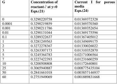
10 1 1 0 -10 0.00000 0 -





Table 4: Effect of the parameter G on the concentration of the reactant in the porous mediacˆ and the current I using Eqns. (21) and (24). B = 0.1, K = 60 and D = 0.1.

G Concentration of

reactantcˆ_{at y=0} Eqn.(21)

Current I for porous media

Eqn.(24)

0 0.3290220758 0.01369372328

0.0001 0.3290219859 0.01369370360

0.001 0.3290211786 0.01369352654

0.01 0.3290131044 0.01369175596

0.1 0.3289322637 0.01367405012

1 0.3281249563 0.01349699175

2 0.3272278367 0.01330026022

3 0.3263307173 0.01310352870

5 0.3245364783 0.02171006564

7 0.3227422393 0.01231660259

10 0.3200508808 0.01172640801

25 0.3065940887 0.008775435104

50 0.2841661018 0.003857146937

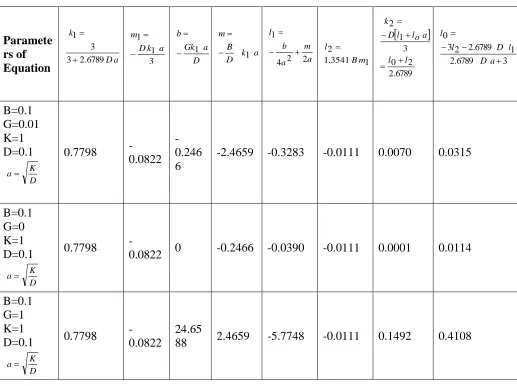
Table 5. Numerical value ofk₁, m₁, b, m , l₁, l₂, k₂, l₀ for various values of parameters B,G,K,D and a

Paramete rs of

Equation Da

k

6789 . 2 3

3 1

 

3 1 1

a k D m

 

D a Gk b

1

 

a k D B m

1

 

a m a b l

2 2 4 1

 



1 3541 . 1

2

m B l 

 

6789 . 2

2 0

3 1 2

l l

a o l l D k

 

 



3 6789

. 2

1 6789 . 2 2 3 0

 

 

a D

l D l

l

B=0.1 G=0.01 K=1 D=0.1

D K a

0.7798

-0.0822 -0.246 6

-2.4659 -0.3283 -0.0111 0.0070 0.0315

B=0.1 G=0 K=1 D=0.1

D K a

0.7798

-0.0822 0 -0.2466 -0.0390 -0.0111 0.0001 0.0114

B=0.1 G=1 K=1 D=0.1

D K a

0.7798

-0.0822

24.65

88 2.4659 -5.7748 -0.0111 0.1492 0.4108

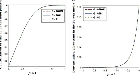
Fig.4 shows that the convection parameter G has no significant effect on the concentration profiles for typical conditions (

G



0 1

.

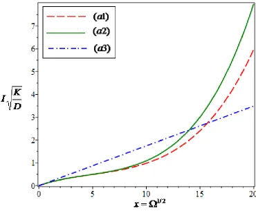
Figure 7. Variation of current I K/Dwith square root of rotation rate 1/2 . Eqn. (35) represents the Levich equation. The typical values of parameters are taken as

follows:

1 2 1

2 2

1 2

0005 . 0 ,

1 . 0 , 1

, 00001 . 0 , 1 , ,

51 .

0          

 x k_r s k mm v mm s h mm D_p D_f mm s



1 , / 05607086 .

41 , 172 0008211214 .

0 , 46 0057310432 .

0

or B hx3 G x2 K  x2 D

(a1) Eqn. (24).

(a2) Eqn. (38) (Where G is a neglected). (a3)Eqn. (35) (Levich equation).

Fig.7 includes the results obtained with the new analytical solution for the PRDE current versus the square root of the rotation rate. Deviations from linearity suggest that a kinetic limitation is involved in the electron-transfer reaction. Equation (35) corresponds to the Levich equation, which is the expression of the current on a flat rotating disk electrode for a mass transfer limited reaction. From this plot it can be concluded that the behaviour of the PRDE current (Eq. (24) with respect to the rotation rate can differ greatly from the Levich current (Eq. (34) or (35)) when 1/215.

Figure 8. Sensitivity of parameters: Percentage change in dimensionless current I whenK60,D0.1,B0.1andG0.1

6.1 Sensitivity

The current on porous rotating disc electrodes depends on the parametersK,D, Band G. A sensitivity analysis is performed based on the differentiation of the aggregated model [29]. Thus, the partial derivative of current (dependent variable) with respect to parameters K,D, B and G

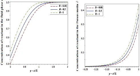
(independent variables) is studied at typical values of these parameters (K60,D0.1,B0.1andG0.1), obtaining the percentage of change of the current. The results are shown in Fig.8 and they point out that parameters D and B have more impact than K and G. These results are consistent with those observed in Figures 3-6.

7. CONCLUSIONS

ACKNOWLEDGEMENT

This work was supported by the Department of Science and Technology, SERB-DST (EMR/2015/002279) Government of India. The Authors are also thankful to Shri J. Ramachandran, Chancellor, Col. Dr. G. Thiruvasagam,Vice-Chancellor, Academy of Maritime Education and Training(AMET), Deemed to be University, for their constant encouragement.

Nomenclature

S.NO SYMBOL UNIT NUMERICAL VALUES

1

c(concentration of reactant in the fluid) mol/cm3 _{0 to 1} 2 cˆ (concentration of the reactant in the

porous media) mol/cm

3 _{-1 to 0}

3  Constant 0.51

4 k _mm2 O(105)

5 kr S1 O(1)

6 v 2 1

S

mm  O(102)

7 Df mm2S1 O(103)

8 Dp mm2S1 O(104)

9 h mm O(101)

10  rpm ₍₁₀3_)(Since,₁₀3_rpm)

11 G/B Dimensionless

parameter

1 2

10 10  

12 B None 102 1

13 _T None 7.018103

14 k_rk/v None ₈₁₀6

15 k/R2 None 2106

16 h/R None 0.125

17 D_f /v None ₂₁₀3

18 D_p/v None _4.4₁₀4

19 DDp/Df None O(101)

20 2kh(/v)3/2 None 2O(102)

21  2k/v None 2

21

3 / 1 f v D 3

      



 1.9610O(101)

23 yz/ Dimensionless

height -

25 G3 /2k(9/2v2Df )1/3 None 15.9946O(105)

26 B 3/22kh(99/v52D4f )1/6 None 3.3826O(102)

27  3kr /(kr /)(9v/2Df )1/3 None 0.0151O(103)

28

D a Gk

b 1 None -

29 k a

D B

m ₁ None -

30

3 a k D

m₁ 1 None -

31

a D 6789 . 2 3

3 k₁



 _{None -}

32





6789 . 2

l l 3

a l l D

k₂  1 o  0 2 None -

33

3 a D 6789 . 2

l D 6789 . 2 l 3

l₀ 2 1

 



 _{None -}

34

D K a , D K

a2   None -

35

a 2

m

a 4

b

l₁ ₂  None -

36 l₂ 1.3541Bm₁ None -

Notation:

c - Concentration of the reactant in the fluid phase

c

ˆ - Concentration of the reactant in the porous media D - Diffusion coefficient

f

D -Diffusion coefficient in the fluid phase p

D -Diffusion coefficient in the porous media kr - First-order reaction rate constant k - Permeability ofthe porous media h - Thickness of the film

r - Radius

 - Rotation rate (angular velocity)

 -Kinematic viscosity

n - Number of electrons in the reaction F - Faraday constant

V - Volume of the disk film R - Radius of disc

APPENDIX A:

Analytical solution of equations (8) and (9) using HPM.





2 2 2 2 2                   dy dc B dy dc y dy c d p dy dc y dy c d p (A1)





2 2 2                      dy c d B dy c d Gy c dy c d D p c dy c d D p (A2) The approximate solution of the equations (8) and (9) are:

. ... p c p c c

c ₀  ₁  ₂ 2  _(A3)

. ... p cˆ p cˆ cˆ

cˆ ₀  ₁  ₂ 2  (A4)

where p is the embedding parameter and p[0,1] Substituting (A3) and (A4) in (A1) and (A2) and equating the like coefficients of p on both sides we get,

0 dy dc y 3 dy c d :

p 2 0

2 0 2

0 _{ }

(A5) 0 D cˆ dy cˆ d : p 0 2 0 2

0 _  _

(A6) 0 dy dc B dy dc y 3 dy c d :

p 2 1 0

2 1 2

1 _{  }

(A7) 0 dy cˆ d B dy cˆ d Gy cˆ dy cˆ d D :

p ₁ 0 0

2 1 2

1 _{   }

(A8)

The boundary condition for the equations (A5) and (A6) are as follows:

 

1, y

c₀ (A9)

 

0, y

cˆ₀ (A10)

0 y ,

cˆ

c₀ ₀  (A11)

0 y at , dy cˆ d D dy

dc_{0  0 }

(A12)

Solving the equation (A5), using the boundary condition (A9),

        3 1

0 ,y

3 1 m 1 ) y ( c  ` (A13) where m₁ is a constant that is determined using the matching boundary condition (A11) and (A12). Solving equation (A6) using the boundary condition (A10),

 

cˆ₀  _{1 (A14)}

where, and k₁

D K

Also, using the boundary conditions, c₀ cˆ₀, aty0and at y 0 dy

cˆ d D dy

dc_{0  0 }

,

1

1 ,0 k

3 1 m

1 

       (A16) a k D m

3 ₁ ₁

 _(A17)

The numerical value ,0 2.6789. 3 1 _      

 Solving equations (A16) and (A17),

3 a k D m , a D 6789 . 2 3 3

k_{1 1} 1





(A18) Now equation (A7) becomes,

0 y , 3 1 dy d Bm dy dc y 3 dy c d ₃ 1 1 2 2 1 2           (A19) such that 3 3 2 3 1

1 ,y k

3 1 k y , 3 2 m B ) y (

c 

                (A20) Using the boundary conditionc₁0 at y, the constantk₃0.

               3 2 3 1

1 ,y

3 1 k y , 3 2 m B ) y (

c  

(A21) where,k₂ is constant. Also,

3 2 1

3

1 _{3exp( y )(Bm y) 3k e} y

dy

dc _{  } 

(A22) 2 0

1 _3k dy dc y    (A23)

Equation (A8) can be written as,

0 dy cˆ d D B dy cˆ d y D G cˆ D K dy cˆ

d _{0 0}

1 2 1 2   

 (A24)

Using equation (A14),





ˆ ˆ 1 2 2 1 2   

a c e b y m

dy c d ay (A25)

where, .

D K a , a k D B m , a k D G

b ₁  ₁  (A26)

ay ay ay ay ay e p a e y m e l a e y b a e y b y

c    ₀   ₁ 

2 2 1 2 4 4 ) (

ˆ (A27)

Using the boundary condition,c₁(y)0 at y, we get, p₁0,

ay ay ay e l a e y b a m a b e y y c ₀ 2 2 1 4 2 4 ) (

ˆ _ 

  



_{ }

 (A28)

The derivative of cˆ₁(y)becomes,



 



4 2 4 ˆ 0 2 2

1 ay ay ay ay ay

ae l e y e a y a b e e a y a m a b dy c

d _{   }

     _{ }  (A29) From the above equation,

a l a m a b dy c d y 0 2 0 1 2 4 ˆ            (A30)

And applying the boundary condition, , at y 0

dy cˆ d D dy dc and 0 y at , cˆ

c₁ ₁  1  1 

we obtain the following equations,

0 2

1 0

2

1 ,0 l (or) B m (1.3541) k (2.6789) l

3 1 k 0 , 3 2 m

B    

               (A31)             _{ } 

 l a

a m a b D k ₀ 2 2 2 4

3 (A32)

Solving the equations (A31) and (A32), we can obtain constants l₀ and k₂(Eqn. (A35)). The expression for the concentration of the reactant in the fluid phase and porous media becomes as follows:                   3 1 3 2 1 1 0 y , 3 2 m B y , 3 1 ) k m ( 1 ) y ( c ) y ( c ) y ( c   (A33) ay ay ay

ay _{y e l e}

a b a m a b e y e k y c y c y c 0 2 2 1 1 0 4 2 4 ) ( ˆ ) ( ˆ ) ( ˆ               (A34)

where the dimensionless constants are





1 1

1 1 2

2 1

0 1 1 2 2 1

3

3 3 2 6789 3 2 6789

3 2 6789

1 3541

2 6789 3 4 2

o

D l l a l l

D k a Gk a

m , k , k , b ,

. D a . D

l . D l B b m K

l , m k a, l , l . B m , a

. D a D a a D

APPENDIX B:

The exact solution of Eqns. (30) and (31).

Let G = 0, B =0 the equations (8) and (9) becomes,

0 dy dc y 3 dy c d ₂ 2 2   (B1) 0 cˆ K dy cˆ d D 2 2   (B2) The exact solution of equation (B1) is,

2 3 3 1 y ) y , 3 / 1 ( y ) y (

c   

(B3) Using the boundary condition, c1, y we get



1 ) y , 3 / 1 ( ) y (

c ₁ 3 

(B4) 1 0 y 3 1 3 dy dc ), y exp( 3 dy

dc _{    }



(B5) The solution of the equation (B2) is,

D y K D y K e e y c  

 _{1 2}

) (

ˆ  

(B6) From the boundary condition, c1, y we get,



D y K 1 e ) y (

cˆ  _(B7)

D K dy cˆ d , D e K dy cˆ d 1 0 y D y K 1      (B8)

Applying the boundary condition, at y 0 , dy

cˆ d D dy

dc _{ }

from (B5) and (B8),

D K D

3 1 1

    (B9) KD

3₁₁



(B10) and from the boundary condition,ccˆ, at y0 we get,

1 1

1

1











(B11) Solving the equation (B10) and (B11),

References

1. G. Rahamathunissa and L. Rajendran, J. Math. Chem., 44 (2008) 849. 2. J.H. He, Int. J. Non Linear Mech., 34 (1999) 699.

3. A.M.Wazwaz, Chem. Phys. Lett., 679 (2017)132. 4. S.H. Chang, Appl. Math. Model., 40(2016) 6805.

5. J.H. He, Comput. Methods Appl. Mech. Eng.,178(1999) 57.

6. J. Saranya, L. Rajendran, L. Wang and C. Fernandez, Chem. Phys. Lett. 662 (2016) 317. 7. A.M.Wazwaz, R. Singh and S. Singh, J.Math. Chem., 54 (2016) 918.

8. J.H. He, Appl. Math. Comput., 135 (2003) 73.

9. S. Ganjefar, S. Rezaei, Appl. Math. Model., 40 (2016) 7062. 10.M.K. Sivasankari, L. Rajendran, Kinet. Catal., 54 (2013) 95.

11.G. Adomian, Solving Frontier Problems of Physics: The Decomposition Method, Kluwer Academic Publishers, (1994) Springer Netherlands, Boston, MA.

12.J.S. Duan, A.M. Wazwaz, R. Rach and J. S. Duan , Appl. Math. Model., 37 (2013) 8687. 13.Abdelhalim Ebaida, Mona D. Aljoufia and A.M. Wazwaz, App. Math. Lett., 46 (2015) 117. 14.A. Vu, Y. Qian and A. Stein, Adv. Energy Mater., 2 (2012) 1056.

15.P. Bai, M.Z. Bazant, D. Zane, M. Pasquali and X. Huang, Nat. Commun., 5 (2014) 474. 16.J.J. Hwang and P.Y. Chen, Int. J. Heat Mass Transf., 49 (2006) 2315.

17.D. Zhao, X. Guo, Y. Gao and F. Gao, ACS Appl. Mater. Interfaces., 4 (2012) 5583. 18.T. Kadyk, D. Bruce and M. Eikerling, Sci. Rep., 6 (2016) 38780..

19.E.O. Barnes, X. Chen, P. Li and R.G. Compton, J. Electroanal. Chem., 720 (2014) 92. 20.C. Punckt, M.A. Pope and I.A. Aksay, J. Phys. Chem., C. 117 (2013) 16076.

21.M.J. Sims, N. V. Rees, E.J.F. Dickinson and R.G. Compton, Sens. Actuators B Chem., 144 (2010) 153.

22.G.P. Keeley and M.E. G Lyons, Int. J. Electrochem. Sci., 4 (2009) 794. 23.D. Menshykau and R.G. Compton, Electroanalysis., 20 (2008) 2387.

24.H.T.H. Chan, E. Kätelhön and R.G. Compton, J. Electroanal. Chem., 799 (2017) 126. 25.B. Nam and R.T. Bonnecaze, J. Electrochem. Soc., 154 (2007) F191.

26.F. Gloaguen, F. Andolfatto, R. Durand and P. Ozil, J. Appl. Electrochem., 24 (1994) 863. 27.D.D. Joseph , Q. J. Mech. Appl. Math. 18 (1965) 325.

28. W. J. Blaedel and Joseph Wang, Anal. Chem.52 (1980) 76-80.

29.M. Rasi, L. Rajendran and A. Subbiah, Sens. Actuators B Chem., 208 (2015) 128.