White Rose Research Online URL for this paper: http://eprints.whiterose.ac.uk/135754/
Version: Accepted Version
Article:
Carrivick, JL orcid.org/0000-0002-9286-5348, Heckmann, T, Turner, A
orcid.org/0000-0002-6098-6313 et al. (1 more author) (2018) An assessment of landform composition and functioning with the first proglacial systems dataset of the central
European Alps. Geomorphology, 321. pp. 117-128. ISSN 0169-555X https://doi.org/10.1016/j.geomorph.2018.08.030
© 2018 Elsevier B.V. This manuscript version is made available under the CC-BY-NC-ND 4.0 license http://creativecommons.org/licenses/by-nc-nd/4.0/.
[email protected] https://eprints.whiterose.ac.uk/
Reuse
This article is distributed under the terms of the Creative Commons Attribution-NonCommercial-NoDerivs (CC BY-NC-ND) licence. This licence only allows you to download this work and share it with others as long as you credit the authors, but you can’t change the article in any way or use it commercially. More
information and the full terms of the licence here: https://creativecommons.org/licenses/
Takedown
If you consider content in White Rose Research Online to be in breach of UK law, please notify us by
1
An assessment of landform composition and functioning with the first
1proglacial systems dataset of the central European Alps
23
Jonathan L. Carrivick1, Tobias Heckmann2, Andy Turner1, Mauro Fischer3 4
5
1School of Geography, University of Leeds, Woodhouse Lane, Leeds, West Yorkshire, LS2 9JT, UK. 6
2Physical Geography, Catholic University of Eichstaett-Ingolstadt, Germany. 7
3 Institute of Geography, University of Bern, Hallerstrasse 12, 3012 Bern, Switzerland. 8
9
correspondence to:
10
Dr. Jonathan Carrivick,
11
Email: [email protected]
12
Tel.: 0113 343 3324
13 14
ABSTRACT
15
Proglacial systems are enlarging as glacier masses decline. They are in a transitory state from
16
glacier-dominated to hillslope and fluvially-dominated geomorphological processes. They are
17
a very important meltwater, sediment and solute source. This study makes the first
18
quantitative, systematic and regional assessment of landform composition and functioning
19
within proglacial systems that have developed in the short term since the Little Ice Age
20
(LIA). Proglacial system extent was thus defined as the area between the LIA moraine ridges
21
and the contemporary glacier. We achieved this assessment via a series of topographic
22
analyses of 10 m resolution digital elevation models (DEMs) covering the central European
23
Alps, specifically of Austria and Switzerland. Across the 2812 proglacial systems that have a
24
combined area of 933 km2,the mean proportional area of each proglacial system that is
25
directly affected by glacial meltwater is 37 %. However, there are examples where there is no
26
glacial meltwater influence whatsoever due to complete disappearance of glaciers since the
27
LIA, and there are examples where > 90% of the proglacial area is probably affected by
28
glacial meltwater. In all of the major drainage basins; the Inn, Drava, Venetian Coast, Po,
29
Rhine, Rhone and Danube, the proportions of the combined land area belonging to each
30
landform class is remarkably similar, with > 10 % fluvial, ~35 % alluvial and debris fans,
31
~50 % moraine ridges and talus/scree, and ~ 10 % bedrock, which will be very helpful for
32
considering estimates of regional sediment yield and denudation rates. We find groupings of
33
the relationship between proglacial system hypsometric index and lithology, and of a slope
34
threshold discriminating between hillslope and fluvial-dominated terrain, both of which we
35
interpret to be due to grain size. We estimate of contemporary total volume loss from all of
36
these proglacial systems of 44 M m3a-1, which equates to a mean of 0.3 mm.a-1 contemporary
37
surface lowering. Overall, these first quantifications of proglacial landform and landscape
38
evolution will be an important basis for inter- and intra-catchment considerations of climate
2
change effects on proglacial systems such as land stability, and changing water, sediment and
40
solute source fluxes. Our datasets are made freely available.
41 42
KEYWORDS
43
proglacial; glacier; landform; meltwater; landscape evolution; hillslope; fluvial
44 45
HIGHLIGHTS
46
Delineation of 2812 proglacial systems in central European Alps of total 933 km2.
47
Glacier meltwater and landform coverage spatially discriminated for each system.
48
Lithological control evident in slope threshold – contributing area analysis.
49
First order estimate of total contemporary volume loss = 44 M m3a-1.
50 51
1. INTRODUCTION
52
Proglacial systems are amongst the most rapidly changing landscapes on Earth. They are
53
progressively increasing in areal extent, and arguably also in instability due to ongoing
54
effects of climate change on glaciers, permafrost and consequent hillslope and fluvial
55
processes (Ballantyne, 2002; Carrivick and Heckmann, 2017). They are a source of water,
56
sediment, solutes (WSS) and hazardous geophysical phenomena, particularly landslides and
57
glacier outburst floods (GLOFs) (e.g. Carrivick and Tweed, 2013). WSS fluxes dictate alpine
58
hillslope and river channel stability, water thermal and chemical regime, biological
59
communities (fish, invertebrates, plants, algae), and ecosystem functions that influence water
60
quality (nutrient and carbon cycling). Proglacial system geomorphological composition and
61
functioning and landscape evolution are therefore of great importance for natural
62
environmental systems and for human activity. Furthermore, alpine proglacial systems in
63
both the European Alps and globally have influence on human and natural systems far
64
beyond the alpine zone. For example, there are 14 million people living in the European
65
alpine arc (Litschauer, 2014) and there are several billion people directly dependent on water
66
from alpine rivers globally. Across Europe, alpine river tributaries contribute up to eight
67
times the water discharge that might be expected given their basin size and thus have been
68
termed the ‘water towers of Europe’ (EEA, 2009; Huss, 2011).
69 70
Proglacial systems are transitioning from being dominated by glacial processes to being more
71
influenced by paraglacial hillslope and fluvial processes (Church and Ryder, 1972;
3
Ballantyne, 2002; Carrivick and Heckmann, 2017). A transitory state implies intense
73
hydrological, geomorphological and ecological dynamics (c.f. Heckmann et al., 2015;
74
Micheletti and Lane, 2017; Delaney et al., 2017; Heckmann and Morche, in press). However,
75
identifying WSS patterns due to these environmental transition(s) is not straight-forward due
76
to spatio-temporal variability and non-linear and stochastic relationships (Bennett et al.,
77
2014). Furthermore, whilst paraglacial activity is generally considered as a set of earth
78
surface processes that are dominant during the transition time period (Carrivick and
79
Heckmann, 2017), changes in hillslope and channel composition or landforms and sediments,
80
and functioning such as connectivity, can alter the relative importance of these hillslope and
81
fluvial processes in space and time (Bennett et al., 2014; Lane et al., 2017).
82 83
Despite the importance of understanding WSS production, pathways and effluxes, studies of
84
geomorphological composition and functioning within proglacial systems have been few and
85
spatio-temporally disparate. Indeed, geomorphological mapping within proglacial systems
86
tends to be conducted either as a basis for field monitoring of water and sediment fluxes (e.g.
87
Beylich et al., 2017), or as a preliminary step towards making targeted close-range field
88
surveys of topographic changes (e.g. Carrivick et al., 2013; Kociuba, 2016). There have been
89
no quantitative efforts to evaluate the geomorphological composition of proglacial systems
90
across a region, nor to evaluate spatial coverage of major geomorphological processes across
91
a mountain range scale region, nor to evaluate likely sediment sources, pathways and sinks
92
within proglacial systems across a region. These three efforts are necessary precursors to
93
regionalising or upscaling field measurements, and more specifically for making quantitative
94
estimates of volume and mass changes within (and exports from) proglacial systems.
95 96
This study therefore aims to make the first comprehensive quantitative, systematic and
97
regional assessment of landform composition and functioning within proglacial systems. We
98
focus on the central European Alps region due to that region having readily-available data
99
and because we have (published) knowledge of some of the catchments in that region, but we
100
advocate the relevance of this work globally.
101 102
2. STUDY AREAS, DATASETS AND METHODS
103 104
2.1 Proglacial zone definition
4
Proglacial systems across the central European Alps analysed in this study are situated in both
106
Austria and Switzerland due to both of those countries having high-resolution (10 m grid cell
107
size or less) seamless digital data availability. Austria glacier outlines for both the Little Ice
108
Age (LIA) and for the contemporary situation were obtained from Fischer et al. (2015a), Groß
109
and Patzelt (2015) and Glaziologie Österreich (2016). A 10 m grid cell size DEM of Austria
110
that had been down-sampled from airborne laser scanner (ALS) data was obtained via Daten
111
Österreichs (2016).
112 113
Swiss glacier outlines for both the LIA considered those of Maisch (2000). For the
114
contemporary (year 2010) situation they were obtained by manual digitization of
high-115
resolution (0.25 m) aerial orthophotographs acquired between 2008 and 2011 (Fischer et al.,
116
2014, 2015b). High-resolution topographic data for Switzerland comprising a 2 m grid cell
117
size, down-sampled to 10 m grid cell size for this study to be comparable to the Austria Digital
118
Elevation Model (DEM), was derived from Airborne Laser Scanning (ALS) as published by
119
Fischer et al. (2014, 2015b).
120 121
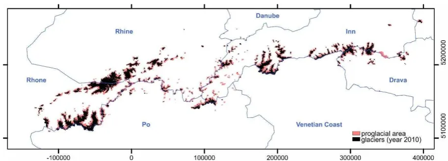
[image:5.595.69.526.399.563.2]122
Figure 1. Spatial coverage of glaciers and proglacial systems across central Europe
123
(Austria and Switzerland) with major drainage basin boundaries (watersheds). Grid
124
coordinates (metres) are projected in UTM zone 33N.
125 126
Proglacial systems across the central European Alps (Fig. 1) were defined automatically by
127
subtracting modern glacier outlines from LIA glacier outlines after Carrivick et al., (accepted).
128
This simple calculation produced a proglacial system extent or boundary, which is necessary
129
for spatial analyses, and a system area (spatial size). In order to minimise misidentifications
130
and extraneous parts of proglacial systems (such as where: (i) some glaciers have reduced in
131
width at relatively high elevations; (ii) some glaciers have reduced in ice extent on plateaux or
132
on cols as a result of fragmentation or disintegration; and, (iii) portions of the landscape
5
presently in transition between ice-marginal and proglacial regimes), we specified a 100 m
134
buffer around the modern outlines and excluded this area from our analyses.
135 136
Geological data was sourced from the International Geological Map of Europe (Asch, 2003;
137
IGME, 2016) and chosen over national level datasets so as to give consistency in mapping
138
and terminology as well as a general-level classification suitable for the regional-scale
139
analysis of this paper.
140 141
With consideration of future use of our results for understanding WSS fluxes from proglacial
142
systems and especially of those transmitted downstream where they affect local populations,
143
hydropower and communications infrastructure, and agriculture we discriminate by major
144
central European drainage basin. These outlines (watersheds) were sourced from the Global
145
Runoff Data Centre (GRDC) www.grdc.de.
146 147
148 149
Figure 2. Example of the spatial discrimination of proglacial systems using glacier
150
outlines from the LIA ‘year 1850’ (Maisch, 2000) and from the present ‘year 2010’ (A),
151
of categories of slope in these systems (B) and of contributing area analysis (C), in this
152
case for the Glacier du Mont Miné and Glacier de Ferpécle area in Switzerland. Shades
6 of blue in panel 1C can be considered to represent a ‘likelihood’ of that grid cell 154
receiving glacial meltwater runoff, being calculated per grid cell as the difference
155
between grids of contributing area with and without glaciers. Grid coordinates are
156
projected in CH1903_LV03.
157 158
2.2 Spatial discrimination of major geomorphological process domains
159
In a first-order classification of proglacial systems based on their topography, we not only
160
calculated statistics of elevations (Fig. 2A) and slopes (Fig. 2B) of all grid cells within each
161
proglacial system, but also the hypsometric index of each as categorised following the Jiskoot
162
et al. (2009) approach where very top heavy hypsometric values indicate much more area at
163
high elevation than at low, and very bottom heavy hypsometric values indicate much more
164
area at low elevation than at high.
165 166
Our spatial discrimination of major geomorphological process domains was achieved in four
167
workflow stages, and was in terms of grid cells that are either predominantly influenced by
168
glacier meltwater, other fluvial (fluid flow) processes, or grid cells that are dominated by
169
hillslope (mostly gravitational) processes.
170 171
Firstly, slope grids (Fig. 2B) were computed and the cell values extracted for each proglacial
172
zone. Secondly, contributing area was determined per grid cell via the D-Infinity flow
173
direction and contributing area algorithms (Tarboton, 1997), as available in the TauDEM
174
(2016) set of tools. These algorithms were chosen to recognise the likelihood of braided river
175
networks in proglacial systems where local slopes are shallow. Contributing area calculations
176
assume that (runoff) contributing area correlates with water discharge. Thus they are not valid
177
for grid cells that might receive runoff from a glacier where discharge is driven by melt and
178
often with significant temporary storage. We therefore differenced grids of contributing area
179
with and without glacier surfaces in them. This calculation discriminated grid cells that
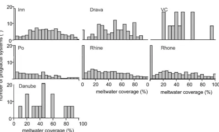
180
cannot receive runoff from glaciers, as coloured greens and reds in figure 2C, versus grid
181
cells that probably do receive runoff from glaciers, as coloured shades of blue in figure 2C.
182
This calculation of the spatial influence of glacial meltwater runoff does not consider flood
183
inundation extent, and we realise flooding is a regular phenomenon in proglacial systems, nor
184
(non-glacial) valley side tributaries.
185 186
After excluding all glacier-meltwater influenced grid cells, we thirdly fitted a polynomial
187
curve with varying numbers of parameters i.e. those of the form:
7
Y = a*(X2) + b*(X) + c (1)
189
where Y = log contributing area, and X = log slope, was fitted to the scatterplot of points of
190
log slope – log contributing area for each proglacial zone using an algorithm provided in the
191
Apache Commons Math library
(https://commons.apache.org/proper/commons-192
math/userguide/fitting.html). For proglacial systems with more than 10 data points and for
193
fitted curves with an identifiable maximum value, the corresponding log slope (X) value was
194
extracted. The automated implementation of this model was via bespoke Java programs
195
which we have made open source and for which we utilised some third party open source
196
libraries as available via: https://github.com/agdturner/FluvioGlacial.
197
Fourthly and finally, conversion of this log percent slope to a degrees slope enabled mapping
198
and calculation of the percentage area of each proglacial zone that is apparently dominated by
199
either fluvial or hillslope processes.
200 201
The percentage area of each proglacial zone dominated by glacial meltwater was calculated
202
similarly, by converting the difference in contributing area (Fig. 2C) to a binary 1 =
203
difference, 0 = no difference, then summing the number of grid cells with a difference and
204
calculating the area of these as a proportion of the total proglacial zone area.
205 206
2.3 Segmentation of major landform types
207
In order to estimate the proportion of different landform types associated with different
208
geomorphological processes, we analysed the probability density function (PDF) of slope as
209
described by Loye et al. (2009). The method assumes slope to be normally distributed on
210
characteristic landform types, and aims at decomposing the observed slope PDF into a
user-211
specified number of normal distributions. The intersections of the resulting PDFs can then be
212
used to discriminate the pertaining landform types. Unlike Loye et al. (2009), we applied the
213
expectation-maximisation algorithm implemented in the R package mixtools (Benaglia et al.,
214
2009; Heckmann et al., 2016) to the slope PDF of a sample (n=25000). We limited this
215
sample to a subarea of the countrywide DEM10, namely to the area covering the proglacial
216
systems plus a 200 m buffer to include adjacent rockwalls, and with glacier-covered areas
217
masked.
218 219
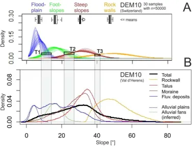
Figure 3A illustrates that the PDFs inferred from the 30 samples are more and more
220
consistent with increasing mode; the largest scatter is evident for the “floodplain” class, while
221
the PDFs representing rockwalls are all very similar. Accordingly, the range of possible
8
intersections of the single landform type PDFs is wider for T1 and T2, and quite narrow for
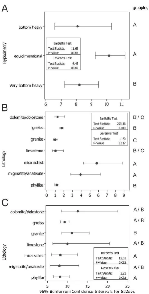
223
T3. Depending on the alpine morphotectonic unit, Loye et al. (2009) reported T3 in the range
224
46° to 54°; intersections at T1 and T2 were not explicitly reported (due to the focus of the
225
paper), but can be extracted from their diagrams: T1=8° to 13°, T2 = 21° to 26°. Note that
226
Loye et al. (2009) used a one metre cell size DEM, so the values of slope are expected to be
227
higher than those computed from our ten metre cell size DEM.
228 229
In order to validate the choice of intersections between each probabilistic group of slope
230
values, we analysed a 10 m cell size DEM of part of the Val d’Hérens (Switzerland), for
231
which Lambiel et al. (2016) have published a digital geomorphological map. We used the
232
polygons of selected landform types to extract the associated PDFs of slope from the DEM
233
(Figure 3B) and we found that the total slope PDF of the Val d’Hérens (thick black curve in
234
Figure 3B) was representative of the slope PDF of proglacial systems that we investigated in
235
the Austrian and Swiss DEMs.
236 237
Regarding the intersections of slope PDFs of different landform types, T3 appears to be
238
consistent with the intersections of the rockwall PDF with the PDFs of “talus” and
239
“moraine”. The slope PDF of “fluvial deposits” in the map is multimodal, probably
240
accounting for floodplains, terraces and alluvial cones of different gradient; therefore, two
241
normal distributions have been fitted visually (the blue and green dashed curves) to the first
242
two modes of the “fluvial deposits” PDF. They intersect with each other in the range of T1
243
(upper panel), and with the “talus” PDF in the range of T2. Based on these observations, we
244
regard our classification as sufficient and set the intersections for discriminating probabilistic
245
slope groups at (a) 7.5°, (b) 18° and (c) 42°.
9 248
[image:10.595.71.453.67.358.2]249
Figure 3. A: Normal distributions of slope for four landform types generated from 30
250
samples of the Swiss DEM (glaciers and areas outside of proglacial areas + 200 m buffer
251
excluded) after Loye et al. (2009, see text for details). The ranges where PDFs intersect
252
are denoted T1 (flood plain footslopes), T2 (footslopes steep slopes) and T3 (steep
253
slopes rock walls). Boxplots show the distribution of corresponding means. B: The
254
intersections of the empirical slope distributions of four landform types of the
255
geomorphological map of Val d’Hérens (Lambiel et al., 2016) are fairly consistent with
256
the ranges T1-T3 indicated in (A). See text for details.
257 258
In order to assess the uncertainty of the intersection values due to sampling and iterative PDF
259
decomposition, we repeated the PDF 30 times. We selected k=4 as the user-specified number
260
of single PDFs, assuming (intuitively) that the following landform types were most
261
representative for proglacial systems: (a) rock walls, (b) steep slopes such as scree and lateral
262
moraines, (c) alluvial or debris cones, and (d) floodplains. We assume that these landform
263
types have markedly different PDFs of slope, and set the following initial means, , and
264
standard deviations, , for the iterative normalmixEM algorithm, based on preliminary
265
analyses of proglacial systems that we are especially familiar with, i.e. Ödenwinkelkees:
266
Carrivick et al. (2013, 2015), and Kaunertal: Heckmann et al. (2016b) as (a) =45°, =3; (b)
267
=30°, =6; (c) =15°, =7; (d) =5°, =12. Moreover, k=4 is consistent with Loye et al.
268
(2009).
10
2.4 Regional relationships of proglacial hypsometry and slope
271
One way analysis of variance (ANOVA) was used to analyse relationships between slope
272
threshold (between hilldominated and fluvially-dominated land, derived from
slope-273
area analysis) with the categorical variables of hypsometric index and lithology. Hypsometric
274
index was also employed as a quantitative variable to compare it in the same manner to
275
lithology. Categories of lithology with less than 10 samples in them (sandstone, amphibolite,
276
carbonates, meat-sediment group, marble, tonalite, sand, claystone) were excluded from the
277
analysis for being not statistically significant. A test for equal variances was performed to
278
identify 95% confidence intervals for the samples within each category. For each of these
279
three relationships statistical groups were identified using Fischer’s individual error rate.
280 281
Our proglacial system outlines and distributed elevation and meltwater influence are made
282
freely available (Carrivick, 2018). The outlines are a shapefile in UTM zone 33N projection
283
and with attributes of drainage basin, HI and percent meltwater influence per system.
284
Distributed elevation enables slope and hence landform classes to be computed quickly as
285
described above in this paper. The meltwater influence grid has been extracted/clipped to
286
proglacial system extent but was computed using a regional DEM. Note that contributing area
287
also requires the regional DEM to be analysed.
288 289
3. RESULTS
290
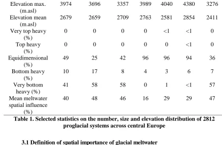
In total we analysed 2812 proglacial systems (Austria: 23 %, Switzerland: 77 %) with a
291
combined area of 933.5 km2 (Table 1). These proglacial systems span a wide geographical
292
area, several climatic and geological regions and a large elevation range. They have
293
hypsometry that is predominantly equidimensional; i.e. a near-equal distribution of area at all
294
elevations (e.g. in the Po, Rhine and Rhone drainage basins), whilst more than half of the
295
proglacial systems within the Drava, Venetian Coast and Danube drainage basins are very
296
bottom heavy, i.e. with much more area situated at lower elevations (Table 1).
297 298
Inn Drava V.Coast Po Rhine Rhone Danube
Number of proglacial
systems
652 117 12 317 794 906 14
Area sum (km2)
307.6 78.8 6.3 78.3 200.2 255.9 6.4
Elevation min. (m.asl)
11
Elevation max. (m.asl)
3974 3696 3357 3989 4040 4380 3276
Elevation mean (m.asl)
2679 2659 2709 2763 2581 2854 2411
Very top heavy (%)
0 0 0 0 <1 <1 0
Top heavy (%)
0 0 0 0 0 <1 0
Equidimensional (%)
49 25 42 96 96 94 36
Bottom heavy (%)
10 17 8 4 3 6 7
Very bottom heavy (%)
41 58 58 0 1 <1 57
Mean meltwater spatial influence
(%)
[image:12.595.64.518.71.368.2]40 48 46 16 29 29 47
Table 1. Selected statistics on the number, size and elevation distribution of 2812
299
proglacial systems across central Europe
300 301
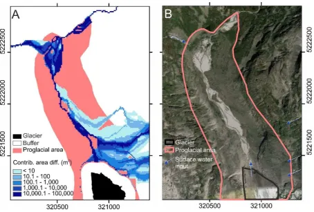
3.1 Definition of spatial importance of glacial meltwater
302
Our spatially-distributed estimate of glacial meltwater influence agrees very well with reality,
303
for example as shown in figure 4 for the Ödenwinkelkees catchment (Carrivick et al., 2013,
304
2015), where glacier-fed, glacier-influenced and groundwater streams create a distinguishable
305
patchwork of (well-studied) streams and rivers (Dickson et al., 2012; Brown et al., 2015).
12 308
[image:13.595.72.527.69.376.2]309
Figure 4. Visual comparison of our contributing area-derived estimate of the spatial
310
coverage and importance of glacier meltwater (A), versus reality (B), as for the
311
Ödenwinkelkees catchment in central Austria, where surface water inputs are from
312
Dickson et al. (2012) and Brown et al. (2015).
313 314
Across all of the central European Alps proglacial systems the mean proportional area of
315
proglacial systems that is probably affected by glacial meltwater is 37 %. However, there is a
316
very wide dispersion to this data (Fig. 5) and we found no relationship between proglacial
317
area size and percentage meltwater influence. Excluding the numerous examples of proglacial
318
systems that apparently have no glacial meltwater influence, most obviously due to complete
319
disappearance of glaciers from these catchments, there is a very large inter-quartile range
320
(IQR) for proglacial systems within the seven drainage basins; specifically from and IQR of
321
19 % (Po) to 55 % (Rhone). The meltwater coverage histogram in Figure 5 for the Inn
322
drainage basin is normally distributed (excluding zeros), whereas those for the Po, Rhine,
323
Rhone are skewed towards lower meltwater coverages, with modal values of ~ 5, 15 and 25
324
%, respectively. The Drava, Venetian Coast and Danube basins have too few proglacial
325
systems for a normality test to be significant. There are a few examples in both countries
326
where virtually the entire area of a proglacial system is probably affected by glacial
327
meltwater.
13 329
[image:14.595.76.522.82.351.2]330
Figure 5. Histograms of meltwater coverage (% of total proglacial system area) for each
331
major drainage basin with headwaters in the central European Alps.
332 333
3.2 Geomorphological functioning: hillslope versus fluvial processes
334
The slope threshold determined from our slope-area analysis for separating
fluvially-335
dominated and hillslope-dominated (mostly gravitational processes) grid cells for each
336
proglacial system hada mean of 27o across the central European Alps. There is no
337
statistically significant difference between the mean slope threshold values for each drainage
338
basin (Table 2) at the 5 % significance level. Slope threshold value histograms for proglacial
339
systems within each of the seven major drainage basins are almost normally-distributed, with
340
the mean and median values very similar (Table 2), although the Venetian Coast and Danube
341
datasets that are too small in number (samples) for any significant distribution to be detected
342
(Fig. 6; Table 2).
14 345
Figure 6. Histograms of the slope threshold discriminating between fluvial and
346
hillslope-dominated grid cells for proglacial systems in the central European Alps.
347 348
Inn Drava V.Coast Po Rhine Rhone Danube
Proglacial systems
with identifiable
slope threshold
(n) 422 86 10 92 300 129 10
Mean 26 24 26 27 27 28 30
Std. dev. 18 18 18 14 18 17 24
Lower
quartile 16 13 17 19 18 22 17
Median 25 22 24 27 26 27 27
Upper
quartile 32 30 42 32 32 34 35
Table 2. Selected descriptive statistics of the slope threshold (degrees) for discriminating
349
between hillslope-dominated and fluvially-dominated terrain
350 351
Analysing the slope threshold for each proglacial zone permitted calculation of the area of
352
each proglacial zone that is predominantly affected by fluvial or by hillslope activity. Overall,
353
35 % of proglacial systems across the central European Alps have > 90 % of their area
354
dominated by hillslope activity and just < 10 % of their area dominated by fluvial activity.
355
There is wide dispersion in this data and we found no difference in the histograms of the
356
percentage area coverage of hillslope activity between major drainage basins. Figure 7A is an
15
example of mapping out grid cells per proglacial zone coloured by whether their slope is
358
above or below the slope threshold for that proglacial zone. This map hints at the similar total
359
spatial coverage of each of the two major process domains. Notwithstanding that many
360
individual systems are hillslope activity-dominated, as mentioned above. the total area that is
361
predominantly controlled by fluvial processes is ~ 472 km2 and the total area corresponding
362
to dominant hillslope processes is ~ 453 km2; i.e. in terms of total proglacial system land area
363
across the central European Alps there is a 50/50 split between fluvial and hillslope
364
dominance.
365
[image:16.595.81.514.240.667.2]366
Figure 7. Results of the slope-contributing area scatterplot analysis to suggest a slope
367
threshold to separate predominant major geomorphological process domains (A), and
368
of PDF analysis on slope values within proglacial systems (A), both displayed in map
369
form for the Gross glockner area of Austria. Relative spatial coverage of each major
370
landform type for each major drainage basin with numbers on top of bars giving
371
absolute area (km2) (C).
16 373
3.3Geomorphological composition
374
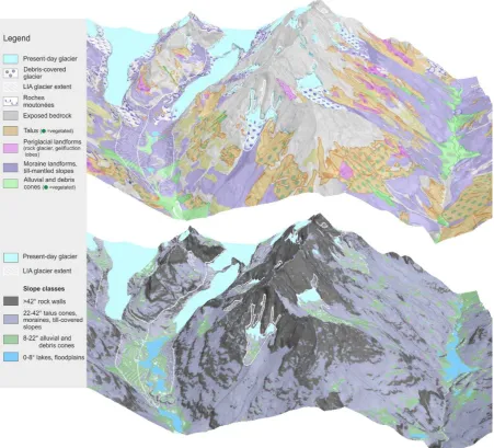
[image:17.595.73.525.131.540.2]375
Figure 8. Three-dimensional perspective visualisation of the Val d’Hérens, Switzerland.
376
The upper part shows a generalised version of a geomorphological map published by
377
Lambiel et al. (2016). The lower panel presents our slope-based classification; the
378
thresholds separating the slope categories were derived from the distribution of slope of
379
the Swiss DEM10 (except present-day glaciers) following Loye et al. (2009), leading to a
380
first-order classification of proglacial systems geomorphology.
381 382
Our slope-based geomorphological classification agrees well visually with reality as
383
measured either from our own experience (Ödenwinkelkees: Carrivick et al., 2013, 2015;
384
Kaunertal: Heckmann et al., 2016) or from published geomorphological maps such as that by
385
Lambiel et al. (2016) for the Val d’Herens (Fig. 8). We attempted a quantitative measurement
386
of the ‘goodness of agreement’ in these figure 8 maps but that was hampered by differences
17
in the mapping, such as Lambiel et al. (2016) did not map rock walls. Figure 7B maps out
388
grid cells coloured by which landform class they belong to, as discriminated by the PDF
389
analysis. This is essentially a rudimentary automated geomorphological mapping with
390
advantages over expert judgement-driven mapping of being fast, repeatable and easily
391
applied across multiple sites and large (mountain range) scales simultaneously. The
392
proportions of the combined proglacial system area belonging to each landform class is
393
remarkably similar between each of the seven major drainage basins, with > 5 % fluvial, ~35
394
% fans, ~50 % moraine ridges and talus/scree, and ~ 10 % bedrock (Fig. 7C).
395 396
3.4 Regional associations and patterns
397
No trend was detected in the slope threshold with east-west or with north-south location
398
across the central European Alps so it is apparently not associated with regional variations
399
such as climate. However, the relationship between slope threshold and hypsometric index
400
identifies two statistically different groups. Specifically, proglacial systems with
401
‘equidimensional’ hypsometry have a slope threshold of mean 22.9 degrees that is
402
statistically different to the mean of 25.3 degrees of proglacial systems with ‘very bottom
403
heavy’ (most area situated at lower elevation) hypsometry. Proglacial systems with bottom
404
heavy hypsometry have a mean slope threshold of 26.4 degrees but the dispersion of the data
405
is sufficiently great for it to belong to both groups, p-value 0.002 (Fig. 9A).
406 407
Three statistically different groups exist between hypsometric index and lithology. Proglacial
408
systems underlain by mica schist, magmatite and marlstone all belong to one group in terms
409
of their slope threshold, gneiss and phyllite belong to a second group, and granite belongs to a
410
third group. We note an association of these three groups with grain size, where group 1
411
rocks are fine/medium-grained, group 2 are medium/coarse-grained, and group 3 has large
412
grains. Statistically, dolomite could belong to either group 2 or 3, p value 0.107 (Fig. 9B).
18 414
[image:19.595.181.421.71.542.2]415
Figure 9. Test for equal variances and identification of statistical groupings of slope
416
threshold discriminating between hillslope- and fluvially-dominated terrain within
417
proglacial systems of each hypsometric class (A), of hypsometric index with lithology
418
(B), and of slope threshold with lithology (C). Note varying x-scale between panels. Note
419
groupings are not transferable between panels.
420 421
Analysis of the relationship between slope threshold and lithology identified two groups; one
422
comprising mica schist and phyllite, which are both very well bedded/foliated metamorphic
423
rocks, and one comprising granite, which is a massive igneous rock. Dolomite, limestone,
424
migmatite and gneiss could all statistically belong to either group and are either crystalline
425
sedimentary or metamorphic rocks (Fig. 9C).A relationship between rock hardness and the
19
slope threshold discriminating between fluvial and hillslope processes (p-value 0.002) is
427
apparently non-linear and most likely so because phyllite and mica-schist are strongly
428
bedded/foliated and across the central European Alps tend to maintain a high angle of
429
inclination (Fig. 9C).
430 431
4. DISCUSSION
432
On the basis of our definition of proglacial systems being most simply represented by land
433
area between LIA and contemporary glacier margins, we discriminate parts of alpine
434
landscapes that have undergone rapid short term evolution. On the basis of a series of
435
geometric measurements alone it was extremely difficult to identify groupings or patterns in
436
topographic metrics of the proglacial systems of the central European Alps. That was a
437
surprise given that proglacial systems are conventionally assumed to be created or at least
438
primarily conditioned by glaciation (Church and Ryder, 1972) and that those glacial
439
processes are dependent on climate-topography interactions (Raper and Braithwaite, 2009),
440
which vary systematically with location across the European Alps. Nonetheless we were able
441
to spatially characterise geomorphological functioning, landform type, meltwater influence
442
and estimate rates of landscape evolution, all of which are precursors to making informed
443
land and water management across Europe in terms of natural hazards, natural resources,
444
habitat and water quality and ecosystem services, for example.
445 446
4.1 Coverage of major geomorphological process domains
447
We have used a slope threshold value of between 24o and 30o (mean 27o) to quickly
448
discriminate geomorphological functioning; hillslope-dominated (mostly gravitational
449
processes) land surfaces that are steeper than that threshold value, versus fluvially-dominated
450
land surfaces that are shallower than that threshold. Throughout the central European Alps
451
and within most of the proglacial systems that we have analysed it is hillslope-dominated
452
land that covers the greater proportion of proglacial systems. This terrain we interpret to
453
represent gravity-driven falls and slumps rather than fluvially-influenced slides and flows. As
454
an aside we emphasise our use of the word ‘dominated’; fluvial processes will occur on
455
slopes steeper than our threshold and hillslope-gravity processes will occur on slopes
456
shallower than our threshold. A predominance of hillslope-dominated land surface(s) implies
457
that greater proportions of proglacial systems are sediment sources and temporary storages,
458
as represented by bedrock cliff falls, debris slumps on talus/scree slopes for example. It
459
follows that the minority of land surface within proglacial systems is fluvially-dominated and
20
therefore comprises major sediment pathways and exports. Our recognition of proglacial
461
systems being hillslope-dominated suggests that that there is an abundant sediment supply, as
462
Maisch et al. (1999) and most recently Schoch et al. (2018) have quantified. Furthermore,
463
these measurements strongly suggest that proglacial systems are most likely to be sediment
464
transport-limited, which has implications for statistical or empirical modelling of sediment
465
transfer (e.g. Bennett et al., 2014; Capt et al., 2016).
466 467
4.2 Landforms
468
Our separation of slope classes identified three statistical boundaries and thus four landform
469
groups. For slopes above the 42o boundary, bedrock is interpreted as a source / generation
470
zone of sediment and also as a landcover that generates instantaneous runoff from rainfall.
471
Talus/scree is the predominant geomorphological entity occupying 26o to 42o slopes and this
472
is a temporary sediment store, initially produced as a paraglacial response soon after
473
deglaciation and destabilisation of surrounding slopes, but then reactivated with additional
474
rockfall (e.g. Kellerer Pirklbauer et al., 2012), debris flows, intense rainfall, permafrost
475
degradation or undercutting by rivers, for example. Another typical landform contained in
476
this slope interval are steep lateral and terminal moraines (although those can maintain slopes
477
much steeper than 42°, c.f. Lukas et al. 2012). Therefore a slope of 26o is interpreted as a
478
good estimate in general of a slope threshold between sediment entrainment zones or scour as
479
represented in gullies, many of which are fan-head. Debris fall deposits, debris flow deposits
480
and alluvial fans occupy slopes between 26o and 8o and from our widespread field campaigns
481
are apparently zones almost entirely of deposition with volumetrically minor reactivation.
482
Thus they are at least in the short term a sediment sink. Indeed it is coalescing fans that
483
commonly intercalate with valley fill (braided river and floodplain deposits) to submerge
484
many alpine valley floors, as we ourselves have observed in the Ödenwinkelkees, Kaunertal
485
and as Lambiel et al. (2016) map for the Val d’Hérens (Fig. 8).
486 487
4.3 Water, sediment and solute (WSS) fluxes
488
WSS sources in proglacial systems comprise glaciers, snow packs, eroding gullies,
re-489
activated fans and river banks. The extremely wide dispersion of values of spatial meltwater
490
influence that we have quantified demonstrates that assumptions of the predominance of
491
glacially-sourced meltwater and fluvially-transported sediment and solute in defining
492
proglacial system character and functioning are rather over-simplifying reality. At least
493
spatially that simplification is apparent, although temporally it is well known that episodic
21
floods can do a lot of geomorphological work (e.g. Warburton, 1990; Staines et al., 2015)
495
despite being restricted to a small proportion of a proglacial system area.
496 497
Our analysis has identified likely glacial meltwater pathways and offers an estimate of the
498
spatial coverage, or importance of this meltwater. That spatial importance could be taken as a
499
first-order indication of the sensitivity of a proglacial system to a (future) change in glacial
500
ice meltwater contribution. Such meltwater sensitivity analyses have recently been performed
501
globally, i.e. per major drainage basin, by Huss and Hock (2018) but they report considerable
502
sub-basin (i.e. inter-catchment) variability. In this study we have demonstrated a quick
503
method for quantifying the spatial coverage, or spatial influence, of glacial meltwater and we
504
have shown that varies enormously between proglacial systems within a region and is
505
independent of any recent change in glacier size. We contend that steeper narrower valleys
506
tend to transmit water and sediment beyond a proglacial system, whereas wider shallower
507
valleys tend to permit sediment deposition and progressive aggradation as glaciers diminish.
508
Such spatial analysis and such system sensitivity analysis are both important for
509
understanding intra- and inter-catchment river channel stability, spatio-temporal water
510
temperature regime (Carrivick et al., 2012) and habitat suitability for a wide range of aquatic
511
and riparian organisms (Milner et al., 2017; Fell et al., 2017).
512 513
4.4 Landscape evolution
514
A slope threshold of ~ 10o was proposed by Palacios et al. (2011) to delimit between debris
515
flow and fluvially-dominated terrain in Meteor Crater. Their value is very much lower than
516
ours for alpine landscapes due to lithology. In the relatively soft (mostly sandstone)
517
sediments of Meteor Crater, debris flows cut gullies and fill in troughs, and fluvial processes
518
deliver more sediment and incise the fine-grained material, so that there is a feedback
519
between these debris flow and fluvial processes and both are necessary for landscape
520
evolution. On harder lithologies, with higher tensile strength, such as are typical across the
521
European central Alps, the work of Sklar and Dietrich (2001, 2006) has shown that debris
522
flows will be the primary mechanism by which bedrock incision occurs on steep slopes after
523
deglaciation. This, they report, means that grain size is a key control on bedrock incision and
524
geomorphological work achieved, which seems to be reinforced by our identification of a link
525
between our slope threshold value and our groupings of lithology (Fig. 9). Indeed, grain size
526
control (and rock hardness and sediment supply) has been used to explain scatter that is
527
common in the tail, the fluvial end, of slope-area power law plots (e.g. our eqn. 1). Landform
22
and landscape evolution is very dependent on sediment supply and there is a critical
529
threshold, which is yet to be ascertained for proglacial systems, whereby too much sediment
530
supply produces land surfaces becoming ‘drowned’, and whereby too little retards abrasion
531
and thus incision. Across the central European Alps Maisch et al. (1999) remarked that
532
sedimentary and mixed sedimentary-rocky glacier beds dominate and so in general sediment
533
supply should be high and valley-fill sediment should persist where topography permits.
534
Valley infill sediments can be detected automatically using low-angle slope filters and as this
535
study has shown major depositional landforms such as alluvial and debris fans can also be
536
discriminated with slope-based analyses.
537 538
4.5 Implications for estimating regional proglacial erosion rates
539
Our maps of meltwater influence, of landforms and of major earth surface processes each
540
offer important information for water and land management, such as characterising
541
(evolving) sediment (and solute) sources, pathways and sinks, hillslope and channel stability
542
and thus habitat character and quality. Together these datasets are several of the components
543
necessary to estimate spatially-distributed (inter-catchment) proglacial geomorphology,
544
which can vary markedly between catchments (e.g. Carrivick and Rushmer, 2009), and erosion
545
rates. However, additional data is required on representative erosion rates for different
546
landform classes and as Carrivick and Heckmann (2017; their figure 10) have shown there
547
are very few direct measurements and a very wide range of values, for each landform class.
548
The recent study by Delaney et al. (2017) emphasises problems within a catchment of levels
549
of detection, over-printing (erosion at a point subsequently obscured by deposition), and of
550
converting volume to mass loss (e.g. with debris-covered ice-cored moraine), even with
well-551
constrained annual DEMs spanning > 25 years.
552 553
To estimate a regional erosion rate, there are problems with applying a relationship from a
554
single proglacial system to all systems because there are many controls on erosion rate other
555
than proglacial area, such as connectivity, area impacted by meltwater etc. Nonetheless, if we
556
assume that the > 25 year data reported in Delaney et al.’s (2017) figure 3 is representative of
557
proglacial systems (spatially and contemporaneously) across the European Alps a polynomial
558
relationship (r2 = 0.96) can be created between volume change and proglacial area (km2).
559
Then it is possible to estimate a contemporary total volume loss of 44,003,800 m3a-1 for all
560
central European proglacial systems combined, which equates to a mean of 0.3 mm.a-1
561
contemporary surface lowering. These mean values are a snapshot and an estimate only. They
23
hide the dominant contributions of fewer larger proglacial systems, although 99 % of all our
563
estimates were < 16 mm.a-1. The mean values are greater than the postglacial erosion rates
564
(surface lowering equiv. 0.15 mm.a-1) calculated by Campbell and Church (2003) and
565
Hoffman et al. (2013) for the Coast Mountains of British Columbia, but an order of
566
magnitude less than suggested by single site analyses within the European Alps of
567
geomorphological evidence (e.g. 30 mm.a-1 to 90 mm.a-1 Curry et al., 2006) and of
multi-568
temporal proglacial DEMs (e.g. 34 mm.a-1: Carrivick et al., 2013). They are several orders of
569
magnitude greater than estimates derived from sedimentation within proglacial lakes or
570
reservoirs (as summarised in Carrivick and Heckmann, 2017) which only capture net material
571
efflux rather than intra-catchment mobility. Nonetheless, they probably represent a good
572
estimate of regionally-averaged contemporary rates, especially given that proglacial systems
573
are rapidly expanding and adjusting to climate change through deglaciation, permafrost
574
degradation and meltwater and precipitation regime shifts.
575 576
5. SUMMARY AND CONCLUSIONS
577
We have presented the first quantification of the topography and geomorphological
578
composition of proglacial systems across the central European Alps, and specifically for 2812
579
sites across Austria and Switzerland. We make these system outlines and distributed
580
elevation data freely available (Carrivick, 2018). We found no association of topographic
581
metrics with location, which we supposed might represent patterns of climatic influence.
582
However, we did find statistically different groups in terms of a relationship between
583
hypsometric index and lithology, and of slope threshold with lithology. Proglacial systems
584
underlain by mica schist, magmatite and marlstone all belong to one group, gneiss and
585
phyllite belong to a second group, and granite belongs to a third group. These relationships
586
suggest that grain size is a key control not only on proglacial system topography but also on
587
the spatial patterning and relative importance of hillslope (mostly gravitational processes)
588
versus fluvial processes and thus on system status as sediment supply- or sediment
transport-589
limited.
590 591
For each proglacial system we have defined the spatial coverage of hillslope versus
valley-592
floor fluvial processes and used these to evaluate the spatial arrangement and importance of
593
likely WSS sources, pathways and sinks. Across the central European Alps the proportions of
594
the total proglacial system area belonging to each landform class is remarkably similar, with
595
> 5 % fluvial, ~35 % fans, ~50 % moraine ridges and talus/scree, and ~ 10 % bedrock.
24
Identification of the spatial occurrence and importance of these landform classes is very
597
helpful for assessing future earth surface processes and landscape stability, such as via
598
sediment yield and denundation rate calculations, for example, as well as for habitat
599
development because these landforms are the local platform upon which mass movements,
600
soil development and biological activity all react to climate change and human-influenced
601
changes. The spatial association, stability and preservation of these landforms changes
602
perhaps most recognisably in terms of surface connectivity, and as micro-topography and
603
micro-climates permit (e.g. Eichel et al., 2016). As a first-order estimate of the contemporary
604
geomorphological activity and thus landscape evolution represented by the spatial coverage
605
of these landform classes, we propose a total volume loss from all these proglacial systems
606
equivalent to a mean of 0.3 m.a-1 surface lowering.
607 608
In conclusion, proglacial systems have become exposed following retreat of glaciers from
609
their LIA margin positions, and have subsequently developed transitioning from
glacier-610
dominated processes to paraglacial processes. Quantifying topographic and
611
geomorphological composition and functioning of proglacial systems is a first and necessary
612
step towards understanding processes driving volume and mass changes within (and exports
613
from) proglacial systems, which themselves are essential for land (stability) and water
614
(quantity and quality) management, hazard analyses and definition of alpine ecosystem
615
services.
616 617
We have presented the first regional scale assessment of proglacial system geomorphological
618
composition and functioning and we have done this in a rapid and efficient manner. Our
619
quantitative analysis can be developed towards providing assessments of alpine landscape
620
sensitivity to climate change, most simply start with spatial analyses considering that the
621
most unstable parts of the landscape are where slope is high and soft sediment is present, and
622
the most stable parts are where slopes are low and soft sediment is absent. Future work on
623
landform evolution within proglacial systems could exploit our datasets for determining
624
sediment distribution and sediment supply across proglacial systems (as opposed to from a
625
glacier), and across alpine landscapes, via multivariate geostatistical modelling (Schoch et al.,
626
2018) and via calculation of spatially-distributed (intra-catchment) sediment budget ratios
627
from repeat DEMs (Heckmann and Vericat, 2018), respectively.
25
REFERENCES
631
Asch, K., 2003. The 1:5 Million International Geological Map of Europe and Adjacent Areas: 632
Development and Implementation of a GIS-enabled Concept; Geologisches Jahrbuch; SA 3, BGR, 633
Hannover (ed.); Schweitzerbart (Stuttgart), 190 p., 45 fig., 46 tab. 634
Ballantyne, C.K., 2002. Paraglacial geomorphology. Quaternary Science Reviews 21:1935-2017. 635
Benaglia, T., Chauveau, D., Hunter, D.R., Young, D., 2009. mixtools: An R Package for Analyzing 636
Finite Mixture Models. Journal of Statistical Software 32, 1-29. 637
Bennett, G.L., Molnar, P., McArdell, B.W., Burlando, P., 2014. A probabilistic sediment cascade 638
model of sediment transfer in the Illgraben. Water Resources Research 50:1225-1244. 639
Beylich, A.A., Laute, K., Storms, J.E., 2017. Contemporary suspended sediment dynamics within two 640
partly glacierized mountain drainage basins in western Norway (Erdalen and Bødalen, inner 641
Nordfjord). Geomorphology 287:126-143. 642
Brown, L.E., Dickson, N.E., Carrivick, J.L. Fuereder, L., 2015. Alpine river ecosystem response to 643
glacial and anthropogenic flow pulses. Freshwater Science 34:1201-1215. 644
Capt, M., Bosson, J.B., Fischer, M., Micheletti, N. and Lambiel, C., 2016. Decadal evolution of a very 645
small heavily debris-covered glacier in an Alpine permafrost environment. Journal of Glaciology 646
62:535-551. 647
Carrivick, J.L., 2018. Contemporary central European proglacial areas. <dataset DOI> 648
Carrivick J.L., Heckmann, T., Fischer, M., Davies, B., (accepted) An inventory of proglacial systems 649
in Austria, Switzerland and across Patagonia. In: Heckmann T, Morche D (Eds) Geomorphology of 650
Proglacial Systems. Landform and Sediment Dynamics in Recently Deglaciated Alpine Landscapes. 651
Springer International Publishing 652
Carrivick, J.L., Heckmann, T., 2017. Short-term geomorphological evolution of proglacial systems. 653
Geomorphology 287:3-28. 654
Carrivick, J.L., Rushmer, E.L., 2009. Inter-and intra-catchment variations in proglacial 655
geomorphology: an example from Franz Josef Glacier and Fox Glacier, New Zealand. Arctic, 656
Antarctic, and Alpine Research 41:18-36. 657
Carrivick, J.L., Berry, K., Geilhausen, M., James, W.H., Williams, C., Brown, L.E., Rippin, D.M., 658
Carver, S.J., 2015. Decadal scale changes of the Ödenwinkelkees, central Austria, suggest increasing 659
control of topography and evolution towards steady state. Geografiska Annaler: Series A, Physical 660
Geography 97:543-562. 661
Carrivick, J.L., Geilhausen, M., Warburton, J., Dickson, N.E., Carver, S.J., Evans, A.J., Brown, L.E., 662
2013. Contemporary geomorphological activity throughout the proglacial area of an alpine catchment. 663
Geomorphology 188:83-95. 664
Carrivick, J.L., Brown, L.E., Hannah, D.M., Turner, A.G., 2012. Numerical modelling of spatio-665
temporal thermal heterogeneity in a complex river system. Journal of Hydrology 414:491-502. 666
Campbell, D., Church, M., 2003. Reconnaissance sediment budgets for Lynn Valley, British 667
Columbia: Holocene and contemporary time scales. Canadian Journal of Earth Sciences 40:701-713. 668
Church, M., Ryder, J.M., 1972. Paraglacial sedimentation: a consideration of fluvial processes 669
conditioned by glaciation. Geological Society of America Bulletin 83:3059-3072. 670
Curry, A.M., Cleasby, V., Zukowskyj, P., 2006. Paraglacial response of steep, sediment mantled 671
slopes to post‘Little Ice Age’ glacier recession in the central Swiss Alps. Journal of Quaternary 672
Science 21:211-225. 673
Daten Österreichs. 2016. Digitales Geländemodell (DGM) Österreich. 674
https://www.data.gv.at/katalog/dataset/b5de6975-417b-4320-afdb-eb2a9e2a1dbf. Last visited March, 675
26 Delaney, I., Bauder, A., Huss, M., Weidmann, Y., 2018. Proglacial erosion rates and processes in a 677
glacierized catchment in the Swiss Alps. Earth Surface Processes and Landforms 43:765-778. 678
Dickson, N.E., Carrivick, J.L., Brown, L.E., 2012. Flow regulation alters alpine river thermal regimes. 679
Journal of Hydrology 464:505-516. 680
EEA., 2009. Regional climate change and adaptation — The Alps facing the challenge of changing 681
water resources. https://www.eea.europa.eu/publications/alps-climate-change-and-adaptation-2009 682
last visited February 2018. 683
Eichel, J., Corenblit, D., Dikau, R., 2016. Conditions for feedbacks between geomorphic and 684
vegetation dynamics on lateral moraine slopes: a biogeomorphic feedback window. Earth Surface 685
Processes and Landforms 41:406-419. 686
Fell, S.C., Carrivick, J.L., Brown, L.E., 2017. The Multitrophic Effects of Climate Change and 687
Glacier Retreat in Mountain Rivers. BioScience 67:897-911. 688
Fischer, M., Huss, M., Barboux, C., Hoelzle, M., 2014. The new Swiss Glacier Inventory SGI2010: 689
relevance of using high-resolution source data in areas dominated by very small glaciers. Arctic, 690
Antarctic, and Alpine Research 46:933-945. 691
Fischer, A., Seiser, B., Stocker-Waldhuber, M., Abermann, J., 2015a. The Austrian Glacier Inventory 692
GI 3, 2006, in ArcGIS (shapefile) format. doi: 10.1594/PANGAEA.844985 693
Fischer, M., Huss, M. Hoelzle, M., 2015b. Surface elevation and mass changes of all Swiss glaciers 694
1980–2010. The Cryosphere 9:525-540. 695
Glaziologie Österreich (2016). Österreichische Gletscherinventare (GI). 696
http://www.glaziologie.at/gletscherinventar.html Last visited March, 2016. 697
Groß, G., Patzelt, G., 2015. The Austrian Glacier Inventory for the Little Ice Age Maximum (GI LIA) 698
in ArcGIS (shapefile) format. doi: 10.1594/PANGAEA.844987 699
Heckmann, T., Morche, D., (Eds) (in press) Geomorphology of Proglacial Systems; Landform and 700
Sediment Dynamics in Recently Deglaciated Alpine Landscapes. Springer International Publishing 701
Heckmann, T., Vericat, D., 2018. Computing spatially distributed sediment delivery ratios: Inferring 702
functional sediment connectivity from repeat high resolution Digital Elevation Models. Earth Surface 703
Processes and Landforms 43: 1547–1554. 704
Heckmann, T., McColl, S., Morche, D., 2016a. Retreating ice: research in pro glacial areas matters. 705
Earth Surface Processes and Landforms 41:271-276. 706
Heckmann, T., Hilger, L., Vehling, L., Becht, M., 2016b. Integrating field measurements, a 707
geomorphological map and stochastic modelling to estimate the spatially distributed rockfall sediment 708
budget of the Upper Kaunertal, Austrian Central Alps. Geomorphology 260:16-31. 709
Hoffmann, T., Müller, T., Johnson, E.A., Martin, Y.E., 2013. Postglacial adjustment of steep, low 710
order drainage basins, Canadian Rocky Mountains. Journal of Geophysical Research: Earth Surface 711
118:2568-2584. 712
Huss, M., 2011. Present and future contribution of glacier storage change to runoff from macroscale 713
drainage basins in Europe. Water Resources Research 47: W07511. 714
Huss, M., Hock, R., 2018. Global-scale hydrological response to future glacier mass loss. Nature 715
Climate Change 8:135-142. 716
IGME (2016). International Geological Map of Europe. 717
http://www.bgr.de/karten/IGME5000/igme5000.htm last visited October 2016. 718
Jiskoot, H., Curran, C.J., Tessler, D.L., Shenton, L.R., 2009. Changes in Clemenceau Icefield and 719
Chaba Group glaciers, Canada, related to hypsometry, tributary detachment, length–slope and area– 720
27 Kellerer Pirklbauer, A., Lieb, G.K., Avian, M., Carrivick, J.L., 2012. Climate change and rock fall 722
events in high mountain areas: Numerous and extensive rock falls in 2007 at Mittlerer Burgstall, 723
Central Austria. Geografiska Annaler: Series A, Physical Geography 94:59-78. 724
Kociuba, W., 2017. Assessment of sediment sources throughout the proglacial area of a small Arctic 725
catchment based on high-resolution digital elevation models. Geomorphology 287:73-89. 726
Lambiel, C., Maillard, B., Kummert, M., Reynard, E., 2016. Geomorphology of the Hérens valley 727
(Swiss Alps). Journal of Maps 12:160-172. 728
Lane, S.N., Bakker, M., Gabbud, C., Micheletti, N., Saugy, J.N., 2017. Sediment export, transient 729
landscape response and catchment-scale connectivity following rapid climate warming and Alpine 730
glacier recession. Geomorphology 277:210-227. 731
Litschauer, 2014. Save the alpine rivers! 732
http://www.ecrr.org/Portals/27/Events/ERRC2014/Presentations/28%20october%202014/session6/ST 733
AR_ERRC_2014.pdf last visited February 2018. 734
Loye, A., Jaboyedoff, M., Pedrazzini, A., 2009. Identification of potential rockfall source areas at a 735
regional scale using a DEM-based geomorphometric analysis. Natural Hazards and Earth System 736
Sciences, 9:1643-1653. 737
Lukas, S., Graf, A., Coray, S., Schlüchter, C., 2012. Genesis, stability and preservation potential of 738
large lateral moraines of Alpine valley glaciers–towards a unifying theory based on Findelengletscher, 739
Switzerland. Quaternary Science Reviews 38:27-48. 740
Maisch, M., 2000. The long-term signal of climate change in the Swiss Alps: Glacier retreat since the 741
end of the Little Ice Age and future ice decay scenarios. Geogr. Fis. Dinam. Quat, 23:139-151. 742
Maisch, M., Haeberli, W., Hoelzle, M.,Wenzel, J., 1999. Occurrence of rocky and sedimentary glacier 743
beds in the Swiss Alps as estimated from glacier-inventory data. Annals of Glaciology 28:231-235. 744
Micheletti, N., Lane, S.N., 2016. Water yield and sediment export in small, partially glaciated Alpine 745
watersheds in a warming climate. Water Resources Research 52:4924-4943. 746
Milner, A.M., Khamis, K., Battin, T.J., Brittain, J.E., Barrand, N.E., Füreder, L., Cauvy-Fraunié, S., 747
Gíslason, G.M., Jacobsen, D., Hannah, D.M., Hodson, A.J., 2017. Glacier shrinkage driving global 748
changes in downstream systems. Proceedings of the National Academy of Sciences 114:9770-9778. 749
Palacios, M.C., Dietrich, W. E, Howard, A., 2011. http://www.ijege.uniroma1.it/rivista/5th-750 international-conference-on-debris-flow-hazards-mitigation-mechanics-prediction-and-751 assessment/topic-3-debris-flow-deposits-and-fan-morphology/the-role-of-debris-flows-in-the-origin-752 and-evolution-of-gully-systems-on-crater-walls-martian-analogs-in-meteor-crater-arizona-usa/ijege-753 11_bs-palucis-et-alii.pdf 754
Schoch, A., Blöthe, J.H., Hoffmann, T., Schrott, L., 2018. Multivariate geostatistical modeling of the 755
spatial sediment distribution in a large scale drainage basin, Upper Rhone, Switzerland. 756
Geomorphology 303:375-392. 757
Sklar, L. S., Dietrich, W. E., 2001. Sediment and rock strength controls on river incision into bedrock. 758
Geology 29: 1087-1090. 759
Sklar, L. S., Dietrich, W. E., 2006. The role of sediment in controlling steady-state bedrock channel 760
slope: Implications of the saltation–abrasion incision model. Geomorphology 82:58-83. 761
Staines, K.E., Carrivick, J.L., Tweed, F.S., Evans, A.J., Russell, A.J., Jóhannesson, T., Roberts, M., 762
2015. A multi dimensional analysis of pro glacial landscape change at Sólheimajökull, southern 763
Iceland. Earth Surface Processes and Landforms 40:809-822. 764
Tarboton, D.G., 1997. A new method for the determination of flow directions and upslope areas in 765
grid digital elevation models. Water Resources Research 33: 309-319. 766
TauDEM (2016). TauDEM documentation - Utah State University. 767