http://eprints.whiterose.ac.uk/150432/
Version: Published Version
Proceedings Paper:
Gardner, P., Rogers, T. orcid.org/0000-0002-3433-3247, Lord, C.
orcid.org/0000-0002-2470-098X et al. (1 more author) (2019) Learning of model
discrepancy for structural dynamics applications using Bayesian history matching. In:
Journal of Physics: Conference Series. XIII International Conference on Recent Advances
in Structural Dynamics (RASD 2019), 15-17 Apr 2019, Valpre, France. IOP Publishing .
https://doi.org/10.1088/1742-6596/1264/1/012052
[email protected] https://eprints.whiterose.ac.uk/
Reuse
This article is distributed under the terms of the Creative Commons Attribution (CC BY) licence. This licence allows you to distribute, remix, tweak, and build upon the work, even commercially, as long as you credit the authors for the original work. More information and the full terms of the licence here:
https://creativecommons.org/licenses/
Takedown
If you consider content in White Rose Research Online to be in breach of UK law, please notify us by
PAPER • OPEN ACCESS
Learning of model discrepancy for structural dynamics applications using
Bayesian history matching
To cite this article: P Gardner et al 2019 J. Phys.: Conf. Ser. 1264 012052
Content from this work may be used under the terms of theCreative Commons Attribution 3.0 licence. Any further distribution of this work must maintain attribution to the author(s) and the title of the work, journal citation and DOI.
Published under licence by IOP Publishing Ltd 1
Learning of model discrepancy for structural
dynamics applications using Bayesian history
matching
P Gardner, T J Rogers, C Lord and R J Barthorpe
University of Sheffield, Department of Mechanical Engineering, Mappin Street, Sheffield S1 3JD, UK
E-mail: [email protected]
Abstract. Calibration of computer models for structural dynamics is often an important task
in creating valid predictions that match observational data. However, calibration alone will lead to biased estimates of system parameters when a mechanism for model discrepancy is not included. The definition of model discrepancy is the mismatch between observational data and the model when the ‘true’ parameters are known. This will occur due to the absence and/or simplification of certain physics in the computer model. Bayesian History Matching (BHM) is a ‘likelihood-free’ method for obtaining calibrated outputs whilst accounting for model discrepancies, typically via an additional variance term. The approach assesses the input space, using an emulator of the complex computer model, and identifies parameter sets that could have plausibly generated the target outputs. In this paper a more informative methodology is outlined where the functional form of the model discrepancy is inferred, improving predictive performance. The algorithm is applied to a case study for a representative five storey building structure with the objective of calibrating outputs of a finite element (FE) model. The results are discussed with appropriate validation metrics that consider the complete distribution.
1. Introduction
Bayesian History Matching (BHM) is a ‘likelihood-free’ method for calibrating computer models (here defined as simulators) under the assumption of model discrepancy, i.e. given the simulator was evaluated with the ‘true’ parameter set there would still be a difference between these predictions and observed data. This is important as without considering this source of uncertainty parameter inferences and output predictions will be biased. The approach is ‘likelihood-free’ meaning that input and output combinations can be removed and added iteratively without invalidating the analysis. Furthermore, this means that the considered parameter domain can be truncated based on physical understanding of the parameters, reducing non-identifiability issues and non-physical inferences.
modelled as Gaussian Processes (GP)s, when a posterior distribution for the parameters is known. The approach is applied to a representative building structure whereby it is shown to be effective in identifying model discrepancy.
2. Bayesian History Matching
BHM seeks to calibrate a statistical model of the form shown in Eq. (1).
zj(x) =ηj(x,θ) +δj+ej (1)
Where zj(x) is the jth observational output given inputs x, ηj(x,θ) is the jth simulator given xand parameters θ. The model discrepancy and observational uncertainty areδj andej respectively. The model assumes that the simulator, discrepancy and observational uncertainty are independent and does not seek to define the model discrepancy’s functional form.
In order to calibrate Eq. (1) the parameter space of the simulator is explored in iterations called waves. During a wave simulator outputs are assessed for different parameter combinations using an implausibility metric and discarded if above a threshold value T. Due to the method requiring assessment of a large parameter space a computationally efficient emulator is utilised reducing the computational burden of evaluating the simulator. Here a GP emulator is implemented; a Bayesian, non-parametric, regression model. A key benefit of using a GP emulator is that it will fit known simulator runs exactly whilst inferring code uncertainty when the emulator predicts away from known simulator runs — in keeping with the brevity of this paper the reader is referred to [8, 9] for more mathematical details on GPs. The GP emulator is constructed as in Eq. (2).
ηj(x,θ)∼ GPj m(x,θ), k((x,θ),(x′,θ′)
(2)
Where the emulator GP prior is defined by a mean m(x,θ) and covariance function
k((x,θ),(x′,θ′)) which have a set of hyperparameters φ
η. The predictive GP emulator mean E(GPj(x,θ)) and code uncertainty, Vc(x,θ) = V(GPj(x,θ)) are then incorporated in an implausibility metric. The formulation stated in Eq. (2) assumes univariate GP emulators for each output, however multivariate GPs could be implemented [10]. The implausibility metric assesses the distance between observations and simulator outputs, weighted by the process’s uncertainties, defined in Eq. (3).
Ij(x,θ) = |
zj(x)−E(GPj(x,θ))| (Vo,j+Vm,j+Vc,j(x,θ))1/2
(3)
Where, Vo, Vm and Vc(x,θ) are the variances associated with the observational, model discrepancy and code uncertainties respectively. By including code uncertainty Vc(x,θ) into Eq. (3) parameter space is retained until the emulator predictions are more certain for that particular parameter region. The observational uncertainty Vo can often be estimated from observational data, although expert judgement may also be used. Model discrepancy uncertainty
Vm can be more challenging to define, but should be elicited from expert judgement.
3
Algorithm 1 Bayesian History Matching for Wave k
θk ∼GMLHC ⊲ Draw parameters from GMLHC
yk=η(x,θk) ⊲ Run the simulator at parameters
Draw nsamplesθks ∼ U min(θk),max(θk)
⊲ Sample parameter space forj = 1 : no. of outputs do
Train and validate GPj x,θk
⊲ Train and validate emulators
E GPj x,θks, Vc,j(x,θks)=GPj x,θks ⊲Predictions at nsamples of θk Calculate Ij(x,θks) ⊲ Assess implausibility of samples
end for
Calcualate Imax(θks)
form= 1 :ndo
if Imax(θks,m)< T then
θknI =θks,m ⊲ Keep non-implausible samples
end if end for
bounds = [min(θknI),max(θknI)] ⊲Obtain new GMLHC bounds if any (Vk
c,j(x,θ)<(Vo,j+Vm,j))orisempty(θknI) then
Stop ⊲ Stop if stopping criteria are met
end if
Eqs. (4) and (5) to collapse the metric to a single value for each parameter combination; where
Vj(x,θ) =Vo,j+Vm,j+Vc,j(x,θ).
Imulti(θ)j = (zj(x)−E(GPj(x,θ)))T(Vj(x,θ))−1(zj(x)−E(GPj(x,θ))) (4)
Imulti(x,θ) = (zj(x)−E(GPj(x∗,θ∗)))T(Vj(x,θ))−1(zj(x)−E(GPj(x∗,θ∗))) (5)
The parameter space is excluded when the implausibility metric is above a thresholdT, where the rejection criteria for a particular parameter combinationθ is defined in Eq. (6).
I(θ) (
≤T ifθ∈θnI,
> T ifθ∈θI
(6)
The threshold value depends on the type of implausibility metric being considered. For individual implausibilitiesIj(x,θ) a sensible thresholdT is Pukelsheim’s 3σrule — stating that any continuous unimodal distribution will contain at least 99.5% of probability mass within three standard deviations away from the mean [12]. For multivariate implausibilities the threshold T
is set as a high percentile (i.e. α > 95%) from a chi-squared distribution with either j or the input size x degrees of freedom, i.e. T = F−1
χ2 (α) — the output from a chi-squared quantile function. This can be thought of as performing a frequentist hypothesis test on the parameter combination, using a chi-squared (χ2) test.
(a) (b)
[image:6.595.77.521.122.419.2](c)
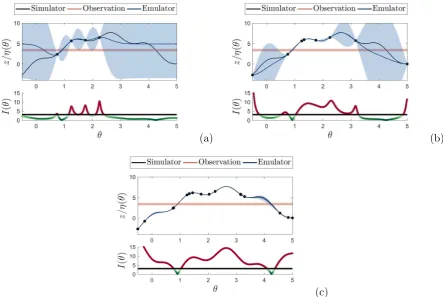
Figure 1. BHM wavesk= 1,2,4 for the numerical example. Top panels show the observational data with ±√Vo+Vm shaded region against the simulator and emulator predictions, trained using the simulator runsη(θk) (·). The bottom panels show the implausibilityI(θks) against the threshold T = 3, where green regions are non-implausible and red implausible. Panel (a), (b) and (c) show waves k= 1,2,4 respectively.
based on the implausibility metric and criteria, with the bounds of the non-implausible region determined. A new wave can then be run with a LHD constructed from these bounds.
Finally, a stopping criteria is constructed, based on two outcomes; all the space is deemed implausible or the emulator variance in the non-implausible region is less than the remaining uncertainties, i.e. Vc,j(x,θnI) < Vo,j +Vm,j, which indicates that the emulator is at least as certain about its predictions as the modeller is with the uncertainties due to model discrepancy and observation variability. The stated approach to BHM can be defined in Algorithm 1.
To illustrate BHM, Algorithm 1 is applied to a simple numerical example — see Fig. 1 (where the sampling stage is replaced with a uniform grid). The examples shows that during each wave new simulator evaluations are added, decreasing the code uncertainty of the emulator. This in turn leads to increased parts of the parameter space begin discarded, until the implausibility metric identifies two non-implausibility regions for this example, i.e. the areas where the simulator crosses the observational uncertainty bounds.
2.1. Approximate Posterior Sampling
5
The technique samples a set of independent draws from an unnormalised proposal distribution
θq ∼ q˜ (where ˜q is the unnormalised proposal) which are subsequently used to form a set of unnormalised weights, shown in Eq. (7). The posterior distribution is then estimated by normalising the weights as presented in Eq. (8).
˜
w(θq) =
p(z|θq)p(θq) ˜
q(θq)
(7)
p(θ|z)≈ 1 w˜(θq) n
Pn
i=1w˜(θq)
(8)
However, as BHM does not involve a likelihood, an approximation is formed as defined in Eq. (9) — the product of multivariate Gaussian distributions over z(x) for the set of inputs
x. This assumes that the sources of uncertainty are approximately normally distributed. The proposal distribution can be formulated as a multivariate Gaussian distribution as presented in Eq. (10).
p(z|θ)≈L(θ) = M Y
j=1
N (z(x)|Ej(GP(x,θ)), Vj(x,θ)) (9)
˜
q(θ) =N (θ|µnI, κΣnI) (10)
WhereµnI and ΣnI are the sample mean and variance-covariance from the non-implausible set after the last wave, and κ is an inflation parameter to ensure good coverage of the space. The choice of priorp(θ) depends on the modellers beliefs from the last wave. However it is often reasonable to assume a constant prior over the final non-implausible set, as it is often a fraction of the original parameter domain. This means the weights in Eq. (8) become ˜w=L(θq)/q˜(θq) where θq are a number of samples from ˜q, with the constant prior essentially truncating the proposal samples to be within the final non-implausible domain.
Lastly the approximate posterior from Eq. (8) can be re-sampled in order generate direct samples from the posterior. This involves drawing Nq samples where the probability of occurrence is defined by the normalised weights w(θq) = ˜w(θq)/n1 Pni=1w˜(θq).
3. Model Discrepancy Inference via Importance Sampling
BHM provides a mechanism for calibrating additive model discrepancy and identifying the approximate parameter posterior. The method does not provide a mechanism for inferring the model discrepancy functional form and correcting output predictions. Here an importance sampling methodology is proposed in order to infer model discrepancy uncertainty, assumed to be distributed as a GP.
Once the approximate posterior distribution is inferred samples θ(i) ∼ p(θ|Z,xz) can be propagated through the emulator such that samples of the calibrated simulator output distribution are obtained p(y(∗i,j)|x∗,yj,xz,θ(i),φˆη,j) — ˆφη,j are the jth emulator’s Maximum Likelihood Estimate (MLE) estimate of the hyperparameters and Z is a matrix of the outputs
zj(x)|j=1:Nout. Here it is assumed that all the emulators accurately capture the simulators functional form meaning the hyperparameters ˆφη,j can be treated as fixed rather than being marginalised; as already assumed within BHM. For this reason ˆφη,j are dropped from notation. The desired calibrated and bias corrected distribution for the jth output is
Algorithm 2 Importance Sampling Model Discrepancy Inference forj= 1 :Nout do
Training; for i= 1 :Ns do
Predictp(y(ji)|yj,xz,θ(i),φˆη,j)
fork= 1 :Nφ do
Sample φ(δ,ji,k)∼q(φ)δ,j ˜
w(ji,k)=p(zj|yj(i),xz,θ(i),φ(δ,ji,k))
end for end for
Normalise weightswj(i,k) = ˜w(ji,k)/PNs i=1
PNφ
k=1w˜ (i,k)
j
Prediction; for i= 1 :Ns do
Predictp(y(∗i,j)|x∗,yj,xz,θ(i),φˆη,j)
fork= 1 :Nφ do
Predict ˆz(∗i,k,j) and Σz(i,k∗,j) from p(z∗(i,k,j)|x∗, Z,yj,xz,θ(i),φ(δ,ji,k))
end for end for
Predict the approximation of p(z∗,j|x∗, Z,yj,xz) via Eqs. (13) and (14)
end for
p(z∗,j|x∗, Z,yj,xz) =
Z Z
p(z∗,j|x∗, Z,yj,xz,θ,φδ,j)p(φδ,j) dφδ
p(θ|Z) dθ (11)
Equation (11) is intractable meaning that approximation methods are required in order to obtain samples from p(z∗,j|x∗, Z,yj,xz). The proposed approach approximates the two integrals in Eq. (11) using importance sampling; although this can also be thought of as Bayesian model averaging [14, 15] — where a set of models are weighted by their evidence.
Importance sampling approximations for the two integrals in Eq. (11) are performed, setting unnormalised proposal distributions for θ and φδ,j. The unnormalised parameter proposal ˜qθ(θ(i)) is defined as the approximate posterior distribution from BHM, such that
θ(i) ∼p(θ|Z,xz) areNsre-sampled parameters, all of which are equally likely, i.e. ˜qθ(θ(i))∝1. The model discrepancy hyperparameter proposal distribution is chosen to be equal to the prior, i.e. ˜qφ(φ(δ,ji,k)) = p(φδ,j(i,k)); where Nφ hyperparameter samples φ(δ,ji,k) are obtained for the ith parameter sample θ(i). These choices of proposal distributions mean that the unnormalised weights become ˜w(ji,k)=p(zj|yj(i),xz,θ(i),φ(δ,ji,k)).
For the jth output the method begins by propagating the ith parameter sample θ(i) ∼
p(θ|Z,xz) through the GP emulator in order to obtain the samples y(ji). Subsequently, for the ith parameter sample, hyperparameter samples φ(δ,ji,k) ∼q˜φ(φ(δ,ji,k)) are used in construct Nφ
GP regression models, mapping from y(ji) to zj. The marginal likelihood of the ith, kth GP model is equal to ˜wj(i,k). This process is repeated such that a set of unnormalised weights and
7
[image:9.595.246.474.109.236.2](a) (b)
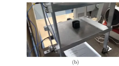
Figure 2. Representative five storey building structure. Panel (a) show the test setup and panel (b) presents an example of the pseudo-damage, added masses, applied to the first floor.
bias corrected predictions, p(z∗,j|x∗, Z,yj,xz), are then approximated as Eq. (12) — where the mean and variance are obtained by the laws of total expectation and variance Eqs. (13) and (14).
p(z∗,j|x∗, Z,yj,xz)≈ N E z∗,j|x∗, Z,yj,xz,V z∗,j|x∗, Z,yj,xz (12)
E z∗,j|x∗, Z,yj,xz =
Ns X
i=1
Nφ X
k=1
wj(i,k)zˆ(∗i,k,j) (13)
V z∗,j|x∗, Z,y
j,xz= Ns X
i=1
Nφ X
k=1
wj(i,k)(Σ(zi,k∗,j)+ ˆz∗(i,k,j)zˆ(∗i,k,j)T)
−E z∗,j|x∗, Z,yj,xzE z∗,j|x∗, Z,yj,xzT (14)
This process is summarised in Algorithm 2. It is noted that other importance sampling based approaches to marginalising the hyperparameters from a GP are adaptive importance sampling [16], where the proposal is iterative amended in order to improve convergence, and Sequential Monte Carlo (SMC) [17]. These techniques could be implemented to provide faster convergence of the approximations.
4. Representative Five Storey Building Structure
Calibration of five bending modes of a representative five storey building structure was performed using BHM in conjunction with the proposed model discrepancy importance sampling approach. Modal testing was performed on the structure made from aluminium 6082 subject to different pseudo-damage extents as shown in Fig. 2. These pseudo-damage extents were added masses
m = {0,0.1, . . . ,0.5}kg fixed to the first floor of the structure demonstrated in Fig. 2b. The structure was excited with 409.6Hz bandwidth Gaussian noise via an electrodynamic shaker, with sample rate and sample time chosen to allow a frequency resolution of 0.05Hz. Accelerometers were placed at each of the five floors in order to obtain the first five bending modes. 40 averages were acquired for each measurement and ten repeats were performed for each damage extent, in order to obtain an understanding of the underlying modal frequency distributions.
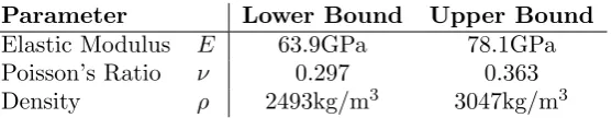
Parameter Lower Bound Upper Bound Elastic Modulus E 63.9GPa 78.1GPa
Poisson’s Ratio ν 0.297 0.363
[image:10.595.162.441.112.166.2]Density ρ 2493kg/m3 3047kg/m3
Table 1. The prior parameter bounds for BHM on the five storey representative building structure.
Uncertainty ω1 ω2 ω3 ω4 ω5
Observational Vo 3×10⁻⁵ 0.02 0.09 0.05 0.01 Model Discrepancy Vm 1.5 0.01 0.01 1 1
Table 2. The process uncertainties defined in the implausibility measure utilised for performing BHM on the five storey representative building structure.
The simulator η(x,θ) was a modal Finite Element Analysis (FEA) model where the five bending natural frequencies were extracted as a set of outputs y. Evaluations of the simulator were acquired for the six damage extents x = {0,0.1, . . . ,0.5}kg and a range of parameter θ
values within a set of prior bounds; set as ±10% of typical material properties for aluminium 6082 as shown in Table 1. Simulator runs for parameter combinations determined by a fifty point, three dimensional GMLHD, were implemented as training data for five independent GP emulators, with a separate ten point three dimensional GMLHD used to generate validation data.
4.1. Bayesian History Matching
BHM was implemented using GMLHDs to provide training data for five independent GP emulators. Each emulator was constructed from linear mean and Mat´ern 3/2 covariance functions. Exploration of the parameter domain was performed via 100,000 samples from uniform distributions over the bounds. A multivariate implausibility (Eq. (4)) was implemented, with the non-implausibility criteria being when the maximum multivariate implausibility for all five outputs (the five natural frequencies) was less than the 99% quantile for a three degree of freedomχ2-distribution (reflecting the size ofxz). The observationalVo,jand model discrepancy
Vm,j uncertainties, set for the first BHM wave are displayed in Table 2 and were estimated from the experimental output variance for the training inputs and from the modeller’s judgement respectively.
The stopping criteria was met after one wave as the code uncertainty for each of the five emulators had an order of magnitude≈10−4. This low level of code uncertainty indicates that
the emulators had captured the simulator behaviour well with diagnostic checks [18] evidencing that the emulators were valid. After the first wave a non-implausible space≈2.3% of the original space was identified.
[image:10.595.148.452.212.252.2]9
[image:11.595.76.512.120.297.2](a) (b)
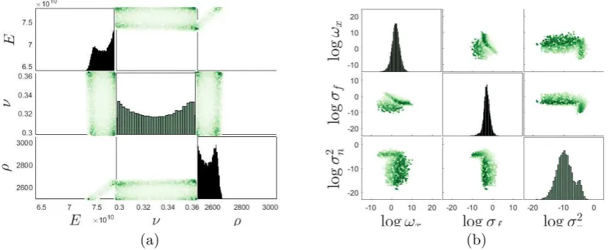
Figure 3. Marginal and pairwise joint posterior distributions for: (a) the parameters identified by the first wave of BHM and (b) the hyperparameters for the fifth natural frequency; where a darker shade represents a higher probability.
and 0.36. These results show the methods ability to account multi-modal behaviour within the defined parameter domain.
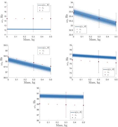
The output distributions for each of the five natural frequencies were obtained via Monte Carlo sampling the posterior parameter distribution. 1,000 samples were taken from the re-sampled parameter posterior distributions and propagated through each of the five emulators in order to obtain realisations of the output distributions. As the code uncertainty across all emulators was extremely low ≈10−4, the emulator mean was taken as deterministic. It is noted
that if the emulator variances were not several orders of magnitude lower than the combined observational and model discrepancy uncertainties to be deemed negligible, posterior sampling of the GP should be implemented (as shown in [19]). The mean predictions of the GP emulators for the 1000 Monte Carlo realisations are presented in Fig. 4 against the observational data used within BHM z(xz) with ±cσ(Vo,j +Vm,j) bounds, where cσ is the standard deviation associated with 99% probability mass of a standard normal (assuming output distributions to be approximately Gaussian). Figure 4 demonstrates that all five outputs are within the defined uncertainty bounds. However, large discrepancies between the experimental observations and simulator (represented by the five emulator’s mean predictions) occur, especially for the first and fifth natural frequencies. This illustrates that the simulator has model form errors, that would lead to incorrect parameter inference if model discrepancy was not considered in the calibration process.
4.2. Model Discrepancy Inference
The proposed importance sampling methodology was applied to the BHM outputs. Here
Nφ = 100 and Ns = 1000, with the model discrepancy GPs being zero mean and Mat´ern 3/2 covariance functions. The hyperparameter priors were Gaussian distributed — logωx,j ∼
N (0,6) (covariance roughness parameter), logσf j2 ∼ N(V(zj),4) (covariance signal variance) and logσ2
nj ∼ N(Vo,j−5,6) (the noise variance) — stating that a low noise and smooth model discrepancy solution is expected.
Figure 4. 1000 samples of the BHM predictive outputs, p(y(∗i,j)|x∗,yj,xz,θ(i),φˆη,j) given
θ(i) ∼ p(θ|Z,xz). The error bars indicate the defined model discrepancy and observation variances.
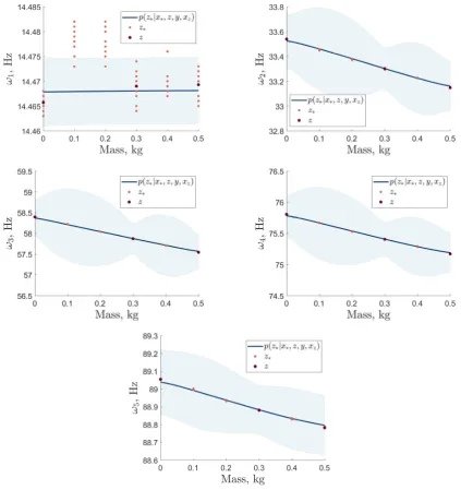
mass states. This is likely due to a lack of information about these point in the training set. It would be expected that with inclusion of these data points predictions would be improved. The posterior distribution over the hyperparameters is estimated from the weights; Fig. 3b demonstrate these distributions for the fifth natural frequency, where the type I and II maximum likelihoods are clearly indicated within the pairwise joint densities, where each refers to the noise and roughness invariant solutions.
11
Figure 5. BHM predictive outputs with the marginalisation of model discrepancy and GP hyperparameters via importance sampling — prior proposal.
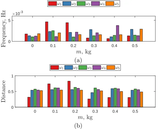
Statistical distance metrics that assess the distance between two distributions were quantified. Firstly, the area metric, the area between the two Cumulative Density Function (CDF)s [20], was applied as shown in Fig. 6a. This metric showed small frequency distances across all predictions, with the 0.1 and 0.2kg mass states for the first natural frequency being the largest. Secondly, Hellinger distances, the integral of the L2-norm between two Probability Density
0 0.1 0.2 0.3 0.4 0.5 0
5 10-3
(a)
0 0.1 0.2 0.3 0.4 0.5
0 0.5 1
[image:14.595.160.438.113.340.2](b)
Figure 6. Statistical distances applied to the bias corrected predictions. Panel (a) are the area metrics when compared to empirical ten point observational CDFs. Panel (b) are the Hellinger distances when compared to KDEs of the observational data. Both metrics are calculated via numerical integration.
5. Conclusions
Model discrepancy must be accounted for, and inferred, when calibrating structural dynamics simulators. This paper presented a BHM methodology for calibrating simulators in the presence of additive, uniform model discrepancy. In addition, an importance sampling based approach has been developed and demonstrated as an effective method for inferring the uncertainty associated with the model discrepancy functional form.
This technique has been applied to a representative five storey building structure where it has been shown to be effective for both calibration and inference of model discrepancy. The importance sampling methodology captured the model discrepancy improving predictive quality for the majority of outputs. However, for the first natural frequency, where the training data was not representative of the functional behaviour, the predictive distributions failed to capture two input points. This would be improved by more informative training data. In addition, due to the high level of uncertainty, the output predictions had a larger variance than the observations leading to large Hellinger distances. These would be improve by increased training observations, or by improving the model form errors within the simulator.
Lastly, further work should be conducted in improving the computationally efficient in the model discrepancy importance sampling. This would allow fewer GP models to be constructed making the approach more practical for scenarios where more observational data is available. Furthermore multivariate GPs should be investigated as priors for the emulators and model discrepancies. This may improve parameter and model discrepancy inferences when there is dependency between outputs.
References
13
[2] Michael Goldstein and Rui Paulo. External Bayesian Analysis for Computer Simulators. Bayesian Statistics 9, (1996), 2012.
[3] Ian Vernon, Michael Goldstein, and Richard Bower. Galaxy Formation: Bayesian History Matching for the Observable Universe. Statistical Science, 29(1):81–90, feb 2014.
[4] Ioannis Andrianakis, Ian R. Vernon, Nicky McCreesh, Trevelyan J. McKinley, Jeremy E. Oakley, Rebecca N. Nsubuga, Michael Goldstein, and Richard G. White. Bayesian History Matching of Complex Infectious Disease Models Using Emulation: A Tutorial and a Case Study on HIV in Uganda. PLoS Computational Biology, 11(1), 2015.
[5] I. Andrianakis, I. Vernon, N. McCreesh, T. J. McKinley, J. E. Oakley, R. N. Nsubuga, M. Goldstein, and R. G. White. History matching of a complex epidemiological model of human immunodeficiency virus transmission by using variance emulation. Journal of the Royal Statistical Society: Series C (Applied Statistics), 66(4):717–740, aug 2017.
[6] Neil R. Edwards, David Cameron, and Jonathan Rougier. Precalibrating an intermediate complexity climate model. Climate Dynamics, 37(7-8):1469–1482, 2011.
[7] Daniel Williamson, Michael Goldstein, Lesley Allison, Adam Blaker, Peter Challenor, Laura Jackson, and Kuniko Yamazaki. History matching for exploring and reducing climate model parameter space using observations and a large perturbed physics ensemble. Climate Dynamics, 41(7-8):1703–1729, 2013. [8] A O’Hagan and JFC Kingman. Curve Fitting and Optimal Design for Prediction. Journal of the Royal
Statistical Society. Series B (Methodological), 40(1):1–42, 1978.
[9] Carl E. Rasmussen and Christopher K. I. Williams. Gaussian processes for machine learning., volume 14. 2004.
[10] Thomas E. Fricker, Jeremy E. Oakley, and Nathan M. Urban. Multivariate Gaussian Process Emulators With Nonseparable Covariance Structures. Technometrics, 55(1):47–56, 2013.
[11] K. Worden, G. Manson, and N. R.J. Fieller. Damage detection using outlier analysis. Journal of Sound and Vibration, 229(3):647–667, 2000.
[12] Pukelsheim. The three sigma rule. American Statistician, 48(2):88–91, 1994.
[13] Holger Dette and Andrey Pepelyshev. Generalized Latin Hypercube Design for Computer Experiments. Technometrics, 52(4):421–429, nov 2010.
[14] Adrian E. Raftery, Tilmann Gneiting, Fadoua Balabdaoui, and Michael Polakowski. Using Bayesian Model Averaging to Calibrate Forecast Ensembles. Monthly Weather Review, 133(5):1155–1174, 2005.
[15] Le Bao, Tilmann Gneiting, Eric P. Grimit, Peter Guttorp, and Adrian E. Raftery. Bias Correction and Bayesian Model Averaging for Ensemble Forecasts of Surface Wind Direction. Monthly Weather Review, 138(5):1811–1821, 2010.
[16] Dejan Petelin, Gasperin Matej, and Vaclav Smidl. Adaptive Importance Sampling for Bayesian Inference in Gaussian Process models. pages 5011–5016, 2014.
[17] Andreas Svensson, Johan Dahlin, and Thomas B. Sch¨on. Marginalizing Gaussian Process Hyperparameters using Sequential Monte Carlo. pages 4–7, 2015.
[18] Leonardo S. Bastos and Anthony O’Hagan. Diagnostics for Gaussian Process Emulators. Technometrics, 51(4):425–438, 2009.
[19] Philipp Hennig and Christian J. Schuler. Entropy Search for Information-Efficient Global Optimization. Journal of Machine Learning Research, 13:1809–1837, dec 2012.
[20] Scott Ferson, William L. Oberkampf, and Lev Ginzburg. Model validation and predictive capability for the thermal challenge problem. Computer Methods in Applied Mechanics and Engineering, 197(29-32):2408– 2430, 2008.