Influence of neighbouring structures on building façade pressures: comparison between full-scale, wind-tunnel, CFD and practitioner guidelines

In

fl

uence of neighbouring structures on building façade pressures:

Comparison between full-scale, wind-tunnel, CFD and

practitioner guidelines

H. Gough

, M.-F. King

, P. Nathan

, C.S.B. Grimmond

, A. Robins

, C.J. Noakes

, Z. Luo

,

J.F. Barlow

a_{Department of Meteorology, University of Reading, United Kingdom} b_{School of Civil Engineering, University of Leeds, United Kingdom}

c_{Department of Mechanical Engineering Sciences, University of Surrey, United Kingdom} d_{School of the Built Environment, University of Reading, United Kingdom}

A R T I C L E I N F O

Keywords:

Façade pressure coefficient Full-scale

Silsoe Wind-tunnel CFD Cubes Ventilation

A B S T R A C T

Façade pressure coefficients are widely used to determine wind-driven ventilation potential for buildings at the design stage. Over nine months we measured façade pressure coefficients under full-scale conditions using the 6 m Silsoe cube in isolation and in a staggered array. Results are compared against a 1:300 wind-tunnel model, a time-dependent computationalfluid dynamics (CFD) model at full-scale and to published pressure coefficients in ventilation design guidance for a range of wind angles.

Across all wind angles, wind-tunnel, CFD and published models tended to underestimate full-scale experi-mental pressure coefficients in magnitude but replicated trends well for a single face on the isolated cube. Agreement was weaker for the array; pressure coefficients are asymmetric with wind direction and results sen-sitive to model set up and measurement strategies. Differences in pressure coefficient across the building compared well in both isolated and array cases, suggesting this is a more robust parameter for models than in-dividual facet data.

It is recommended that building symmetry and surrounding areas should be considered when relying on ventilation guidelines. Scale and computational models are effective to support design for more complex cases; however, it is important to ensure measurement locations are representative and that uncertainties are quantified.

1. Introduction

Predicting ventilation potential in naturally ventilated buildings is a key component in designing buildings that effectively support occupant health and comfort (Wang et al., 2008). However, building geometry, orientation, the thermal environment and local wind conditions make ventilation calculations complex (Chiu and Etheridge, 2007). In urban environments, where a building may be surrounded by neighbouring buildings, the localflowfields may significantly impact the potential effective ventilation rate. Current methods for designing wind driven natural ventilation rely on the knowledge of pressures across the building façade to relate external wind speed, wind angle and openings with ventilation rates (Etheridge, 2002). As such, appropriate pressure data for the building is necessary in order to make reliable assumptions at the

design stage.

Traditionally, during the design stage of large buildings, scale models (including some surrounding buildings) are placed in a wind tunnel and the pressure distributions around the building are measured for various incident wind directions. The resulting pressure coefficients (Cp) can then be used to calculate theflow through ventilation openings at different locations on the façade, using the orifice equation to relateflow rate to wind speed (CIBSE, 2018). Such approaches are also used to produce genericCpdata for different building geometries that are published in the design guidance (CIBSE, 2005) and can be used to carry out ventilation calculations on simpler buildings. These scale-model approaches rely on several assumptions and uncertainties are not always given (Chiu and Etheridge, 2007;Chu et al., 2009). Even for a simple building geometry, wind-inducedflows can be complex and transient (Coceal et al., 2006),

* Corresponding author. Department of Meteorology, University of Reading, Earley Gate, PO Box 243, Reading, RG6 6BB, UK.

E-mail address:[email protected](H. Gough).

Contents lists available atScienceDirect

Journal of Wind Engineering & Industrial Aerodynamics

journal homepage:www.elsevier.com/locate/jweia

https://doi.org/10.1016/j.jweia.2019.03.011

Received 19 December 2018; Received in revised form 8 March 2019; Accepted 9 March 2019

and therefore predicting ventilation rates is difficult. The relation be-tween external and indoor airflow is still an area of much debate around appropriate ventilation prediction strategies (Liddament, 1996) and challenging research due to the lack of full-scale building data (Blocken, 2014). Such limitations motivated the present study.

2. Background

The pressure coefficient (Cp) is a function of the difference between pressure measured on a building's surface and the reference static pres-sure (Δp), the density of the oncoming air (ρ) and the referenceflow velocity (Uref):

Cp¼ _0:5Δ_ρp_U2 ref

(1)

DefiningUrefis complex in an urban area as local wind velocities are wind direction dependent and often only airport data, some distance outside the city, are available. Defining a suitable reference static pres-sure may also be difficult.

Three main methods are used to obtainCpvalues, ventilation rates and airflow characteristics around buildings: full-scale measurements (e.g. Caciolo et al., 2011; Belleri et al., 2014), scale modelling (e.g. Karava et al., 2006; Zaki et al., 2012) and more recently, the use of Computational Fluid Dynamics (CFD) simulations (e.g. Coceal et al., 2007; van Hooff and Blocken, 2013). Often two methods are used in conjunction such as wind-tunnel measurements and CFD simulations (e.g.Yang et al., 2006;Blocken et al., 2012).

The widespread dependence on scale and CFD models highlights the lack of full-scale data available for evaluation of the results. Some fea-tures may not be captured at smaller scales (Richards and Hoxey, 2007). All methods have advantages and disadvantages, with full-scale and scale measurements being costly in terms of personnel and equipment, and CFD models limited by the computational power available, especially if the area of interest is large. CFD and scale models need to be tested against full-scale data to ensure that the model is representative of the full-scaleflow and captures allflow features.

Data are often representative of a specific building and may not be applicable to other structures. With a variety of building designs, loca-tions and research objectives, it is difficult to inter-compare data and as such datasets are not widely utilised by industry. Different building types have been studied, for example, stadia (van Hooff and Blocken, 2010), hospitals (Gilkeson et al., 2013) and schools (Bako-Bir o and Clements-Croome, 2012). Large differences inflow behaviour are found for open, sheltered and courtyard situations within close vicinity (Gao et al., 2012), and the need to use local reference measurements is evident. The urban environment provides particular challenges for predicting the natural ventilation of a specific building, due to the large number of influencing factors on theflow (Dobre et al., 2005), such as: the location of the reference wind speed and direction, local wind speed and direc-tion, wakes of neighbouring buildings, localised heating and cooling and the relative position of neighbouring buildings.

Buildings are often simplified into arrays of cubes in order to reduce model complexity, improve understanding of complexflow features both within and above the cubes and to model how the morphometry of the array affectsflow (Coceal and Belcher, 2004;Coceal et al., 2007;Wood et al., 2009;Carpentieri and Robins, 2015).

Pressure coefficients have been measured at full-scale on individual cubes including work using a 2.4 m cube (Maruyama et al., 2008) and the 6 m Silsoe metal cube (Straw et al., 2000;Yang et al., 2006;Kasperski and Hoxey, 2008;Richards and Hoxey, 2012). However very little work has considered building arrays at full scale. More common is the use of uniform arrays of blocks in a wind tunnel measuring pressure coefficients to infer ventilation rate (Zaki et al., 2012), although non-uniform buildings (Li et al., 2015) are also used along with scale models of real buildings.

This study was conducted as part of the RCC (REFRESH Cube Campaign) project (Gough et al., 2018a) and aims to compare facade pressure data collected at full-scale to both a 1:300 scale wind tunnel model and transient CFD simulations for both an isolated cube and a cube within a limited irregular nine cube array. The full-scale setting allows for detailed investigation into external airflows and the exploration of the influence of wind speed, wind angle and the effect of neighbouring structures on surface façade pressures. Research into the different ventilation measurement methods and influence of the array on cross ventilation using the full-scale site and a CFD simulation are published (Gough et al., 2018a,2018b;King et al., 2017a). The RCC has also been used to explore the effectiveness of using a GPU Lattice-Boltzmann CFD model to simulate urban airflow (King et al., 2017b).

This is thefirst study to systematically compare the three different modelling approaches across all wind angles with a comprehensive full-scale dataset for both an idealised isolated case and urban array case. The results are also compared with the current UK and international pre-vailing wind pressure coefficient design guidelines published by ASH-RAE, AIVC and CIBSE. We aim to provide a better understanding of how to use scale and CFD modelling approaches effectively and provide insight into the application of guidelines for real-world design.

3. Methods

3.1. Full-scalefield campaign (RCC-FS)

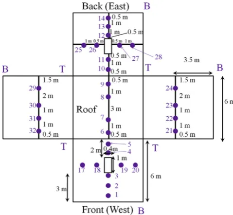
An overview of the RCC–REFRESH cube campaign is given byGough et al. (2018a)and is detailed extensively in Gough (2017). Full-scale observations were undertaken using a cubic test structure (Fig. 1) located at Wrest Park, Silsoe, Bedfordshire, UK (52.01088N, Longitude 0.4121W). From 9th October 2014 to 10th April 2015 a staggered asymmetric array was in place. The isolated cube was studied from 30th May 2015 to 7th July 2015. The instrumented cube (dimensions 6 m6 m6 m) was clad inflat, steel sheets to ensure uniform external surfaces. The front and back faces had removable panels (0.4 m wide by 1 m high, centre point 3.5 m from the ground) so the cube could be both a sealed and a ventilated structure.

Although the surroundings were not uniform there were no topo-graphic features which uniquely affect the site conditions. To the west, farmer'sfields with crop stumps (circa 0.1 m in height) were present. The site is well-characterised (Gough et al., 2018b) and was previously modelled both in the wind tunnel (Richards and Hoxey, 2007) and by CFD (Yang et al., 2006;King et al., 2017a). Nearby structures include two storage tanks (~2 m high and 4 m wide, black triangle,Fig. 1) and a storage shed (black diamond,Fig. 1), which was roughly the same height as the instrumented cube (6 m) 15 m wide and 25 m long with a sloping roof.

An asymmetric staggered array of eight 6 m straw cubes was built around the instrumented cube (Fig. 1). Although the sides and tops of the cubes were not completely smooth, given the focus on meanflow trends, this roughness is assumed to have little, if any, effect on Cp values measured at the test cube. Within the total area of the array (1260 m2) the plan area density (λp) was 25.7% (Fig. 1). The array faced into the expected prevailing wind direction of approximately 240, this is referred to as 0hereafter (Fig. 1).

(2010). The sonic anemometers were inter-compared before and after the experiment; as no drift and minimal differences were observed, no inter-instrument corrections are made.

The cube surface pressure was measured using pressure taps: 7 mm holes located centrally on 0.6 m2steel panels, which were mountedflush onto the cube cladding to minimise their effect on the pressures measured (Fig. 2). Pressure signals were transmitted pneumatically, using 6 mm internal diameter plastic tubes to transducers within the cube. The individual transducers meant that the pressure tap measure-ments were simultaneous at 10 Hz. Honeywell 163PC01D75 differential pressure sensors (pressure taps 1–16) had a range of2.5 inches of H2O

(~498 Pa). Pressure taps 17–32 were Honeywell 163PC01D76 differ-ential pressure sensors and had a range of 5 inches of H2O

(~1245 Pa). All pressure sensors had a manufacturer stated response time of 1 ms.

30 external pressure taps were used with 2 internal pressure taps, as Straw (2000)notes that the internal pressures may vary over time. The 30 external pressure taps used were split across the four faces; four on the roof, four in a horizontal array on the centre line across the North and South faces and nine on the front and back faces, withfive of those in a vertical array and four in a horizontal array (Fig. 2). A reference pressure was measured using a static pressure probe (in house, Richards and Hoxey, 2012), with a reference dynamic pressure measured using a directional pitot tube (in house) at 6 m (building height) alongside the 6 m reference sonic anemometer (Fig. 1). Errors in pressure tap mea-surements are discussed inGough et al. (2018b).

3.2. Wind tunnel set up and measurement technique (WT-RCC)

Scale model experiments of the RCC (RCC-WT) were conducted in the Environmental Flow Research Centre (EnFlo), University of Surrey‘A’ wind tunnel (low speed open circuit). The test section is 0.6 m high, 0.9 m wide and 4.5 m long and is constructed of wood and metal with glass side panels. The roof was weighted down to ensure a proper seal and was constructed from a combination of wood and a movable acetate sheet.

The entirefloor of the working section was lined with 6 mm boards covered in a staggered pattern of small right-angled brackets, 8 mm wide (in the spanwise direction) and 2 mm high, previously used bySnyder and Castro (2002), creating rough surface conditions similar to those of the full-scale site. A Perspex turntable (radius 0.15 m) was set into the roughness boards and centred 2.1 m from theflow inlet (Fig. 3). The wind tunnel angle notation follows that ofFig. 1c (bold font).

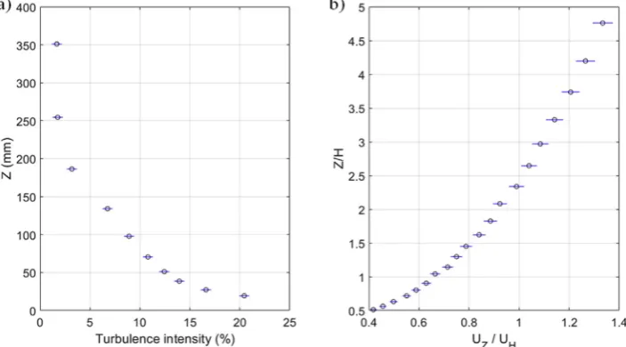
Seven 0.25 mIrwin (1981)spires were used to generate the boundary layer and the height difference between the tunnelfloor and the spires was minimised by using a small metal ramp. The boundary layer thick-ness, measured at 5 points, was 0.15 m above the turntable, with a 0.036 m deep logarithmic layer. The average turbulence intensity at building height of 19%1% is within this error for all tests (Fig. 4). A longitudinal turbulence intensity of 20% at building height was specified byRichards et al. (2001)for the full-scale cube in selected wind condi-tions and in near neutral condicondi-tions (no uncertainty is stated). For the

Fig. 1. RCC full-scale (RCC-FS) study site at Silsoe: a) plan view of main features (unchanged since 2009); b) oblique view into the prevailing wind direction of the cube array, with sonic anemometer locations (text in white background, instruments images in black boxes), storage shed (black diamond) and sewage tanks (black triangle); and c) plan of site with angle notation. The metal cube in (b) and brighter square in (c) are the instrumented cube. Italic angles are meteorological (real) wind angles, with bold angles denoting the naming convention used in this paper. Note that the wide-angle lens distorts the pe-riphery of images. Copyright 2016 Infoterra, Blue Sky Limited and Google Earth. (Gough et al., 2018a,b). (For interpretation of the references to colour in this

figure legend, the reader is referred to the Web version of this article.)

Fig. 2. Location of the pressure taps during RCC on each face of the cube (T,

full-scale site the value of turbulence intensity differs with wind direction (Gough, 2017;Gough et al., 2018a).

The average roughness length (z0) calculated using data within the logarithmic layer for this campaign was 3.3105m1106m (0.0330.001 mm). With a model scale of 1:300, this is equivalent to a full-scale z0 of 0.0115 m0.0003 m (11.5 mm0.3 mm) suggesting

open andflat terrain with a few isolated obstacles and a combination of grass and low crops (Stull, 1988). Given the full-scale site (Section3.1)z0 of 0.006–0.01 m (Richards and Hoxey, 2007), this is regarded as repre-sentative despite the slightly higher wind tunnel value compared to full-scale site. The generated boundary layer (Fig. 4) was found to be similar (within 10%) of the boundary layer used in wind tunnel testing by Richards and Hoxey (2007)and the full-scale measurements from by Richards et al. (2001).

The isothermal wind tunnel simulation neither accounts for the ef-fects of the tree avenue, nearby buildings and woodland at the full-scale site (Fig. 1) nor does it capture the larger turbulence scales due to changing atmospheric stability. The storage shed (Fig. 1) was modelled in the wind tunnel using measurements fromRichardson and Blackmore (1995)and was included for both the isolated and array cases. More detail on the wind tunnel experiments can be found inGough (2017).

The 1:300 scale model of the staggered array, with the pressure tapped cube, was centred on the turntable (Fig. 3). The test section blockage was negligible. The remaining elements were sanded wooden blocks of height 20 mm, previously used byCheng et al. (2007)(Fig. 3). The 20 mm pressure tapped brass cube (also used byCheng et al., 2007) had 42 pressure taps on two opposing sides (referred to as‘front’

and‘back’), with 3 rows of 7 pressure taps on each face (Fig. 5). The height of these rows is different for the two faces, so the cube can be rotated by 180to give 42 pressure measurements on each face. Rotating the cube by 90allows for the pressure data to be captured for the cube sides (‘north’and‘south’in line with the full-scale orientation). The error in the wind direction caused by this rotation was found to be2. Details of the pressure tap measurement setup are included in the Appendix. The reference static pressure was measured at x¼55 mm (0 mm is the centre of the cube), y¼95 mm and z¼300 mm (behind the turntable and in the free stream above cube height) to ensure that it did not disrupt theflow around the array and provided a local reference pressure measurement.

3.3. CFD methodology (RCC-CFD)

A transient Navier-Stokesfinite-volume simulation was used to model the isolated cube and array at full-scale (RCC-CFD) in Ansys Fluent 17.1 (Ansys Canonsburg, PA, USA). The model used a k-ωshear stress trans-port (SST) scale adaptive simulation (SAS) turbulence model, which is a hybrid RANS-LES model that has shown superior results to the more commonly applied steady state RANS model; this is described for this purpose inKing et al. (2017a,b).

A domain based on the full-scale site of (20 m50 m18 m) was modelled with approximately 3Hupstream and 5Hdownstream for the isolated cube as described inKing et al. (2017a,b). The CFD simulation did not include openings in the cube. This bounding is a balance between a dense mesh to maintain the spectral content and the required computing time in order to avoid the decay of turbulent structures. A

Fig. 3. Wind tunnel set up of a) roughness elements, brass cube and Perspex turntable with scales marked and b) the 1:300 scale RCC-WT array.

Fig. 4. a) Average longitudinal turbulence intensity profile for the wind tunnel boundary layer and b) generated boundary layer within the wind tunnel, normalised by

bounding box of 12H168H6H(72 m108 m36 m) was used to account for the larger size of the array.Fig. 6shows the computational domain and mesh characteristics close to the Silsoe cube in the array context. From mesh sensitivity analysis (King et al., 2017a) a grid sizing of 0.01Hat the cube was sufficient to resolve velocity at the side of the isolated cube to within 5% of that measured byHoxey and Richards (1993). Bulkflow cell size increases up to H/10 downstream of the cubes. Final cell counts for the isolated and array cases were ~1.8 million and ~4.3 million respectively. Yþ(a dimensionless variable based onfirst cell size compared to airspeed in thefirst cell) requirements close to the wall are that of URANS: a value of between 35 and 50 was obtained for a grid wall spacing of 0.06 m at the wall.

Site velocity profile measurements are well matched by a logarithmic profile (Richards and Hoxey, 2002):

UðzÞ ¼u_κ*ln

z z0

(2)

FollowingRichards and Hoxey (2002), a reference velocity (Uref) of 2 m s1at z¼6 m and ground roughness lengthz0of 0.01 m were used to define the inlet wind condition. u*

is the turbulent friction velocity (0.13 m s1) andκis von Karman's constant (0.41) (Tu et al., 2018). Inlet turbulence kinetic energy (k) is modelled using (Tu et al., 2018):

k¼ u*2ffiffiffiffiffiffi

Cμ

p (3)

whereCμis the eddy viscosity constant of 0.09. The specific dissipation rate εis based on the turbulent dissipation rateω, given by standard formulations (Richards and Hoxey, 1993):

ε¼_κðzu_þ*3_z

0Þ; (4)

ω¼ ε

kβ* (5)

whereβ*_{is 0.09 (van Hooff et al., 2017).}

Ground roughness length is set to 0.01 m. Sides and top of the domain are modelled as free-slip walls and are far enough away not to impact the

flow around the cube. This is tested by a sensitivity analysis following Blocken and Gualtieri (2012). The downwind outlet is 0 Pa gauge pres-sure in all cases with zero gradient for all other variables. The modelled approachflow velocity profile is similar to the measurements taken at the site byRichards and Hoxey (2002), though errors were not provided.

A second-order upwind scheme is applied to convective terms and a central differencing scheme is applied to diffusion terms. For time inte-gration, a central bounded second-order accurate scheme is utilised. A Courant-Friedrichs-Levy number of 0.08 is used throughout based on Δt¼0.0025,Uref¼2 m s1andΔx¼0.06 m, which is within the range of best-practice used in transient flow simulations (Nozu et al., 2008; Tominaga et al., 2008). An initial steady state simulation is run to create a starting point for the transient simulation using the SIMPLE pressure-velocity coupling scheme (Tu et al., 2018). Pressure interpola-tion, convective terms and the viscous terms of the governing equations are solved with second order discretisation. The transient simulation, using the PISO scheme, is run initially for the amount of time it takes a parcel of air at the inlet to reach the outlet (1 air turn over time) (Tu et al., 2018). The simulations are averaged for 18,000 time steps which cor-responds to aflow time of 45 s. This is sufficient to obtain statistically steady results, as verified by monitoring the evolution of the mean pressure on the Silsoe cube front face using moving averages. Pressure is measured at 10,000 points on each face. Reference pressure is measured at the equivalent location to the reference mast in the full-scale study (Fig. 1).

Fig. 5. Pressure tap measurement points a) used in the wind tunnel. The cube had to be rotated in order to capture 42 points for each face, front side (triangles) and

back side (circles) of the cube, and points matching the full-scale cube are circled (Fig. 1), and b) the 20 mm pressure tapped cube in the wind tunnel.

4. Results

To ensure that the calculated pressure coefficients are unaffected by instrument sensitivity, only full-scale 30 min averages with near neutral stability (0.1<jz/Lj<0.1, wherez/Lis the Obukhov stability param-eter) and a reference wind speed at 6 mUref>3 m s1are used in line with limitations of the pressure tap response time (Richards and Hoxey, 2012). The wind direction (θref) at 6 m is used unless otherwise stated (Fig. 1).

Full-scale measurement errors are derived from instrument error. For wind tunnel measurements the standard error of the averaged data is taken and for CFD data errors are based on the standard deviation over the sampling period of the measurement. All methods use the full-scale

field site co-ordinate system, with a perpendicular wind direction being 0(Fig. 1).

4.1. Comparison of CFD, wind tunnel (WT), full-scale (FS) isolated cube Cpvalues and previous work

To establish whether the current work (RCC) can be considered representative of previous work, Cpvalues measured and modelled for

the isolated cube forθref¼05are compared to: full-scale Cpvalues

previously measured on the Silsoe cube byRichards et al. (2001), an isolated cube in an atmospheric boundary layer (Castro and Robins, 1977) and a 1:40 Silsoe cube model (Richards and Hoxey, 2007). The data digitized from papers have an additional error of ~2%. CFD data are subsampled to 100 points across the vertical line from the front to the back of the cube.

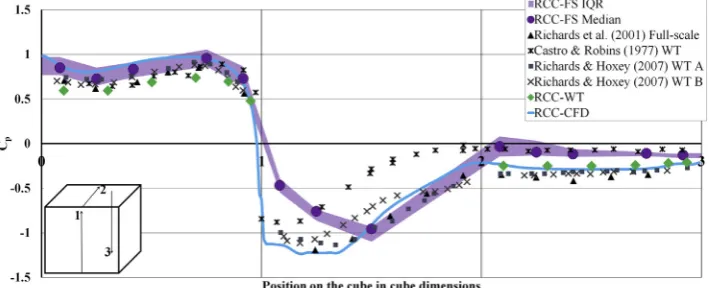
For the front face, the vertical trend in Cpis similar for all datasets

(Fig. 7). The RCC-CFD simulation predicts the highest front face pres-sures, which fall within the range observed at full-scale (RCC-FS), but both are higher than RCC-WT.Richards et al. (2001)compared several studies (both WT and FS) and found a spread in the front face Cpof 0.2,

and thus RCC-WT is in a similar range to the other studies. Suggested causes for the spread were Reynolds number and relative roughness ef-fects (Richards et al., 2001). For this wind direction (θref¼0,Fig. 1), the RCC-FS pressures on both the front and back faces are different to those ofRichards et al. (2001); this may be due to the small number of samples (12 h of 10 min averages for one wind direction) obtained byRichards et al. (2001), meaning it is difficult to determine how representative the case study is of Cpforθref¼05.

The RCC-FS results show good agreement with WT data fromCastro and Robins (1977)for the front and back faces, perhaps due to the their model including a boundary layer meant to simulate the suburban environment, making it more representative of the conditions experi-enced in the full-scalefield for extended periods of time (Fig. 7). The results fromCastro and Robins (1977)have smaller magnitude negative pressure coefficients on the roof of the cube, potentially because the boundary layer and roughness elements upstream produce different wind

shear and turbulence levels at roof height. Roof Cp values are sensitive to the upstream turbulence and the ratio of the cube to the boundary layer depth (Castro and Robins, 1977). For the back face (Fig. 7), the RCC-CFD data agrees better with RCC-WT than RCC-FS data, and lies within the spread of other results, found by (Richards et al., 2001) to be 0.4. The RCC-FS data shows good agreement withCastro and Robins (1977).

The slightly smaller magnitude Cpvalues for the RCC-WT experiment

may be due to the difference in the reference pressure measurement placement and thus the resultant pressure difference.Castro and Robins (1977)andRichards and Hoxey (2007)measured the reference pressure upstream whereas the reference pressure is taken adjacent to the brass cube in the RCC-WT experiment. The reference pressure for the RCC-FS experiment may also be sensitive to wind direction.

Overall, RCC data from all three sources agrees well with previous data in areas where there is small spread–clearly, on the roof there is a large difference between all studies. Bias exists for the back face, where FS data agrees best withCastro and Robins (1977), and CFD and WT data fall within the spread of other studies. Data included here covers a wide range of experimental conditions, with differing turbulence intensities and locations of reference pressure measurements.

4.2. Methodology for comparison of the different datasets

Data availability are quite different for the three data sources. Notably the sample points per face vary between 10,000 for the CFD (potentially unlimited), 42 for the WT and only 9 points in a cross shape for the FS cube (Fig. 2). Thus, features may not be captured by the sparse FS measurement distribution. It is also important to note that U and turbulence intensity vary between the data-sets leading to associated uncertainty in the comparisons.

For the FS front face averageCpis a 30-min arithmetic mean of the 9 pressure from taps forUrefat 6 m (Gough, 2017;Gough et al., 2018a). These are also binned and averaged in 5sectors. Similarly, averages for the WT and CFD data are determined for the 9 FS locations (Fig. 5a) but are 2-min and 45 s averages, respectively. The effect of the array on the pressure coefficient and ventilation rates are discussed inGough et al. (2018a). Here the focus is on the difference between modelling methods and available data.

ASHRAE (American Society of Heating, Refrigerating and Air-Conditioning Engineers, AIVC (Air Infiltration and Ventilation Centre), and CIBSE (Chartered Institute of Building Services Engineers) each have published data for the front face of an isolated building. The CIBSE (CIBSE Guide A, 2018) values are fromLiddament (1996)but corrected from earlier editions. AIVC data are from bothLiddament (1996)and Heijmans and Wouters (2002). ASHRAE's data are based onSwami and Chadra (1988)but has similarities to the AIVC data as both have their origins inWiren (1983). AIVC use three sheltering categories, whereas ASHRAE (Swami and Chadra, 1988) average into one value.Swami and Chadra (1988) adjusted their data around the Cp value measured at

Fig. 7. Comparison of the measured mean

θref¼0 but do not provide the raw measurements before the

adjust-ments in the ASHRAE guidance. The ‘modified’ Swami and Chadra (1988)values (ASHRAE data) treat the cube faces in isolation, whereas Heijmans and Wouters (2002)measure the front, back and sides simul-taneously, capturing the interacting effects of the faces. In standards, wind direction is often split into 45 sectors (CIBSE, 2018,ASHRAE, 2009) with the predicted pressure coefficient of a surrounding building being dependent on a sheltering factor.

Comparison of front faceCpfor the array case is made with the CIBSE 0_{Urban sheltered building’ in the AM10 report (CIBSE, 2018). The} Shielding condition given is‘highly sheltered (i.e. surrounded by ob-structions equivalent to the full height of the building)’(CIBSE, 2018). The front and back face magnitudes are impacted by the reference pressure location but have similar trends. Using front-back differences in Cpmitigates this effect.

4.3. Inter-comparison of RCC full-scale (FS), wind tunnel (WT), CFD and guidelines for the isolated and array cases under various wind directions

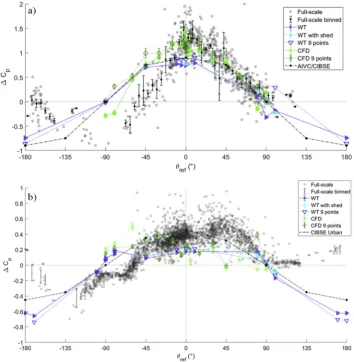
For the isolated cube (Fig. 8a), the 42-point RCC-WT data resembles the FS results, with both having similar trends on the front face: a maximum Cp for θref¼0, a minimum for parallel flow (θref¼90),

becoming negative forθref¼ 90–180. The effect of the storage shed (Fig. 1) can clearly be seen forθref¼90, bringing WT results closer to the

FS measurements, although there are fewer FS data points for this wind direction. There is a large spread of Cp(0.6–1.3) for the FS isolated cube

when exposed toθref¼05. The meanCpfor thisθrefrange is 0.85, with

99.7% of the data being within 0.850.45. Using only nine points on the wind tunnel cube face increases the calculated Cpforθref¼0by 0.1 with little, if any, change for the other measured wind directions regardless of whether the model shed is included.

The RCC-CFD model captures the magnitude of the full-scale results to a greater extent than the wind tunnel, however, it overestimates the drop in front face averagedCpfromθref¼45–90. The Cpvalues are close

to that of the 42-point RCC-WT model forθref¼90 and90(Fig. 8a). The 9-point RCC-CFD data have a larger front faceCpforθref¼0–45, but the difference between the full and 9-point CFD datasets decrease asθref

increases. This suggests that the patterns of negative pressure occurring on the front face forθref¼45–90are much smaller in spatial extent or

weaker in magnitude in RCC-FS than the CFD or WT models.

TheCpvalues for the FS isolated cube are higher, and fall within the 80% bounds set bySwami and Chadra (1988)(ASHRAE) only for some directions between 180<θref<90. Both the AIVC/CIBSE and

ASHRAE results are in good agreement with the RCC-WT results. TheCp minimum is predicted by the AIVC model to occur atθref¼ 90, when

the oncomingflow is parallel. The ASHRAE (Swami and Chadra, 1988) model predicts the minimum value ofCpto occur atθref¼115, when the

flow is impacting on the back face. The minimum binned value for the isolated Silsoe cube occurs aroundθref¼- 90and 115.

For the array case (Fig. 8b) the front faceCpaverages for RCC-WT agree best with RCC-FS data nearθref¼0and 170but show distinctly different patterns with changingθref, notably remaining negative for all

Fig. 8. Comparison of the RCC full-scale (FS)

other angles. Within RCC-WT (cf. to RCC-FS) the trend withθrefis almost

a mirror image, showing that local wind patterns causing suction on the cube are very sensitive to the differences between full-scale and wind tunnelflows. For the array case the inclusion of the storage shed (Fig. 1) in the wind tunnel model has less impact than for the isolated case, the largest change being less than 0.1 aroundθref¼90.

The RCC-CFD data with all sampled points lies mostly within the scatter of the FS data for90 <θref<45, though it is notable how

sensitive this result is to sampling: the 9 point CFD data switches sign, and is closer to the wind tunnel results fromθref¼ 10 to - 60. This

implies that the pressure pattern for90<θref<0is broadly correctly

simulated by the CFD, but the detail of the pattern, when sampled at only 9 points, is displaced, or gradients are sharper than at FS. In the CFD and WT models the tree avenue in this sector (Fig. 1) is not included which could introduce higher roughness and more variability in wind direction

that“smears”out sharp pressure gradients in 30 min averaged FS data.

For θref¼ 90, 45 and 90 there is agreement between the wind

tunnel and the 9-point CFD model. The large negative deviation of RCC-CFD with all datapoints for 60 and 80 suggests that there is large suction towards the corners of the cube that is unrealistic–the 9-point sub-sampling agrees better with FS or WT data.

The RCC-FS and RCC-WT difference for the back face of the isolated cube (Fig. 9a) is likely related to the differing positions of the reference pressure between techniques. A more reduced pressure on the front face corresponds to a lower (i.e. more negative) pressure on the back face, causing an offset for each method. The peak in RCC-WT of 0.5 that occurs at θref¼180 is similar in magnitude to the front face at θref¼0

(Fig. 7a). The full-scale site is also affected by the varying terrain and upstream roughness elements not modelled in the wind tunnel, leading to the clear asymmetry (Fig. 7a). Using 9-point sub-sampled WT data, the back-face Cpforθref¼180increases by 0.1, as seen for the front face at θref¼0, and Cpdecreases by 0.2 forθref¼100(Fig. 9a). Otherwise the

results remain similar. RCC-CFD follows the wind tunnel results for the isolated back face, tending to underpredict by 0.05–0.1, though this difference increases to 0.25 forθref¼75and75likely due to mesh

limitations at this angle (Figs. 9a and6). It is thought that using an adaptive mesh may resolve this and is part of the future work planned with this dataset. CIBSE pressure coefficients for the back face are similar to WT and CFD forθref¼090andθref¼180for the isolated cube,

with the guidelines capturing a similar trend to both WT and CFD, but not FS.

The results of the back face for the array for all methods (Fig. 9b) are similar to the back face of the isolated cube (Fig. 9a). This might be ex-pected as back face of the cube is always on the edge of the array, and thus less affected by the presence of other cubes. The effect of the storage shed on the WT results is less pronounced for the array than for the isolated case, similar to the front face. The RCC-WT and RCC-CFD back face data agree better with RCC-FS than for the front face (Fig. 8b). The 9-point average WT Cpis larger by up to 0.05 for all wind directions but

shape of the curve remains the same. Similarly, sub-sampling the CFD data makes only small differences, suggesting that there might be weaker pressure gradients across the back face.

WT and CFD diverge atθref¼90. This may be related to the storage

shed being not in the CFD model. For the array case the spike in CFD Cpat

θref¼45, is thought to be caused by the mesh size being too large at the

point offlow impact, thus changing the wake and the back faceCp(Figs. 6 and8). Data fromCIBSE (2018)for the sheltered case predicts similar trends to the WT and CFD, like for the isolated case, though magnitudes diverge atθref¼180.

For both the isolated (Fig. 9a) and array (Fig. 9b) back faces the WT model gives symmetrical results withθref, unlike the FS results which are

impacted by the changing roughness with wind direction from obstacles not modelled within the wind tunnel (Section3.2). The CFD results do not show symmetry for the array back face (Fig. 9b) and capture the trend in FS for more negative values for positiveθref. The CIBSE sheltered Cp

values predict similar trends to the WT and CFD for the array case and like for the isolated back face, the magnitudes diverge atθref¼180.

Overall, it is harder to obtain agreement between all three methods for the Cpfront and back face averages for a cube in an array, due to greater

sensitivity of pressure patterns to inevitable differences inflow detail. The difference between face averaged front and back Cp(Fig. 10) is

widely used to predict ventilation rate through openings. Note that this form of presentation is independent of the choice of reference pressure. For the isolated cube the difference is underpredicted by RCC-WT data, though adding the shed improves agreement around 90and using only nine points increases the similarity with RCC-FS data forθref¼0 and

120(Fig. 10a).CIBSE 2018data agrees most with the RCC-WT 9-point data in magnitude and trend. There is little FS data forθref¼ 180but

the wind tunnel data seems to overestimate the peak. Large scatter in the FS results are likely associated with the variable wind directions within the averaging times for both the isolated (Fig. 9a) and array (Fig. 10b)Cp differences. The CFD results lie within the FS scatter from 20 <

θref<90, and sub-sampling to 9 points improves this agreement. The

CFD data shows a symmetrical trend rather than the slight asymmetry seen in the FS data, which is consistent with increased roughness due to the tree avenue decreasing the pressure drop on the cube for70<

θref<20.

For the array case, for45<θref<90the WT results underestimate ΔCp, only capturing some of the lower FS measurements and showing poor agreement atθref¼ 180(Fig. 10b). The CFD results show more

variability and sub-sampling the data reverses the trend with direction, suggesting again that there are sharp gradients in the pressure patterns. The lack of agreement aroundθref¼ 90with FS data for both WT and

CFD shows a localflow at FS that reverses the sign of the pressure dif-ference. However, for θref¼0 45, the CIBSE sheltering data best

agrees with the FS data, before following the trends of the WT and CFD forθref<-90andθref>90. Overall, there is better agreement forΔCp than for individual facets.

5. Discussion

Uniquely, RCC provides a very thorough case study of both isolated and array configurations with three methods from which several impli-cations emerge. The study shows that representing an isolated building as a cube can lead to good agreement (within 25%) between FS, WT and CFD methods to determine pressures across the façade of the building. All three methods show the same trends, and differences are explained by assumptions about boundary conditions, data sampling, and domain limitations. Comparison between the three methods in the array case shows much more mixed results, and the model set up and sampling

strategies have a much more significant influence on the results (differ-ence in values range from 20% to over 200%, especially for oblique angles).

Differences between the three methods (FS, WT, CFD) can be infl u-enced by the number and location of measurement points (Costola et al., 2009). For example, close to cube edges measurement points were ab-sent at FS but preab-sent in the WT and CFD models. For the isolated case, using the 9-point sub-sampling with the WT and CFD model data showed greater similarity (difference reduced by ~10%) to the full-scale results for the front face. This suggests that for better agreement be-tween methods, matching the locations of measurement points is important (Figs. 8and9). However, for the array case, sub-sampling data on individual facets for CFD showed mixed results, with the 9-point sampling agreeing with the WT results but the full CFD data set showing better comparison to FS under certain wind angles. Where WT or CFD models are created to aid interpretation of full-scale data, care must be taken to compare pressure patterns as well as point measure-ments, otherwise they risk becoming misleading, e.g. right pattern, wrong location.

FS results for both the isolated cube and the array show some asymmetry (Fig. 7). This may be caused by the tree avenue (Fig. 1) acting as a windbreak to the oncomingflow, reducing overall wind speed and increasing the turbulence intensity for this wind.

Some differences between the three data sets can be related to up-stream boundary conditions,flow profile and turbulence intensity. The addition of a nearby obstacle in the WT and CFD models generally improvedCpvalues (reduction of 5–15% in the difference in methods) compared to FS. Domain size limitations preclude inclusion of larger obstacles or changes in surface roughness further away. The results imply that cube pressures are sensitive to the correct choice of upstream wind profile even for the array. There is evidence that variability from large scales of turbulence (10%–100%) at FS cause“smearing out”of pressure patterns that are hard to match with WT and CFD models as they generally assume lower turbulence intensity (~20%). As the CFD tur-bulence generator is not truly random some of the pressure variation may be caused by vortex generation rather than a cascade of eddies. For both WT and CFD, the size of the eddies is limited by the domain dimensions. These results imply that future studies should focus on building pressure patterns when exposed to lateralfluctuations or high turbulence intensity as these are more representative of urbanflows.

Individual facet pressure patterns are very hard to match between methods due to great sensitivity of WT and CFD models to details of local

flow and boundary conditions. However, the total pressure drop across the cube, ΔCp, for both WT and CFD is better matched in trend and magnitude to the full-scale data compared to face averaged Cp. In terms

of designing ventilation for real buildings in urban areas, comparison of an individual facet with guideline datasets are reasonable for isolated but poor for the array case, but much improved (reduction of up to 75% of the difference depending on wind angle) when consideringΔCp. As a

practical conclusion, guidelines might advise that this variable be used to estimate the magnitude of pressure drop, and local building layouts with respect to the prevailing wind direction assessed to determine the likely sign on each building facet; i.e. if a building wall faces into the local prevailing wind direction in a neighbourhood it is likely to experience positive pressures.

Comparisons to the guideline data were limited by lack of collection and analysis details. Guidance data needs to be accompanied by more information on how it was created, so that the user can assess its appli-cability, or presented with likely error margins as done in the ASHRAE guidelines. Much of the guideline data are from wind tunnel experiments so lack variable wind conditions of full-scale measurements. It is important to capture the range of variability in pressure coefficients from different building layouts, neighbourhood densities, etc. This could be tackled by systematic experiments (e.g.Hall and Spanton, 2012).

6. Conclusions

Current methods for designing wind-driven natural ventilation rely on the knowledge of pressures across the building façade. As part of the REFRESH Cube Campaign (RCC) project (Gough et al., 2018a), facade pressure data collected at full-scale over a full range of wind conditions are compared to a 1:300 scale wind tunnel model and CFD simulations for both an idealised isolated cube and a cube array representing an urban neighbourhood. This is thefirst study to systematically compare different modelling approaches using a very comprehensive full-scale dataset. From this thorough case study, several implications emerge for modelling and design guidelines.

Within the full-scale dataset there is a large amount of variability in Cp that is not currently seen in the other methods. The wind tunnel (WT), CFD and full-scale (FS) pressure coefficients (Cp) of the isolated RCC cube agree well (within 25% difference) with previous FS (Richards et al., 2001) and WT data (Castro and Robins, 1977;Richards and Hoxey, 2007) measured with the wind normal to the cube. There is good agreement within scatter for the front face (Cpdifference of 0.2–0.7), whilst there

are large but understood differences amongst all studies for the roof (range of 0.7 for Cpvalues). Bias exists for the back face, where FS data

agrees best withCastro and Robins (1977), and CFD and WT data fall within the spread of other studies. The differences in sampling Urefand

Prefalso contribute to differences between methods.

RCCCpfrom WT, CFD and FS are compared for isolated and array cases across the full range of wind angles. Agreement is best for the isolated cube front face, and weaker for the back face (isolated, array) and front face in the array case. For the isolated case, sub-sampling of WT and CFD pressure data to match the location of the 9 taps at FS leads to a reduction of 10% of the difference in Cpfor the front face and made little

difference for the back face. For the array case, sub-sampling of CFD data for the front face leads to different results. These results suggest that matching measured data points is important when comparing methods, but pressure patterns should be compared as well as individual points, especially when they are placed near strong gradients. Adding nearby obstacles caused a reduction of 5–15% in the difference between FS and WT Cpand differences between data for certain wind directions suggest

that matching upstream FS wind profiles and turbulence intensity is important, even for the array case.

The difference between front and back,ΔCp, is compared as this is used in practice to predict cross ventilation rate. For the isolated cube agreement between methods is good for a range of oncoming wind di-rections, with WT and CFD only overestimating values in a wind direc-tion sector known to have increased roughness at FS. For the array case WT and CFD data are in much better agreement but slightly underesti-mate FS values. This suggests that whilst individual façade pressures may be biased by details of WT or CFD modelling set-up,ΔCpis a more robust variable to compare for both isolated and array cases.

Comparison of front faceCpfor all RCC methods with ASHRAE, AIVC and CIBSE guideline data has good trend agreement for the isolated cube, with most WT and CFD datapoints lying within the 80% bounds set by Swami and Chadra (1988)(ASHRAE) and FS data being mostly higher than the guideline data. For the array case there is poor trend agreement as the guideline data are derived using a sheltering factor and do not account for asymmetrical arrays. However, theCIBSE 2018data capture the magnitude ofΔCp well for both the isolated and array cases. Our results suggest that representing a general building in an urban neigh-bourhood through a single pressure data set is not appropriate as the real building orientation, neighbourhood density and height will have a considerable influence on the actual pressures experienced on the façade. Guideline data for buildings within a neighbourhood cannot be“one size

Impact

Façade pressure coefficients in a staggered array are dependent on wind direction and are asymetrical due to sheltering effects. This is not captured in current ventilation design guidelines. An extensive dataset comprising full-scale, wind tunnel and Computational Fluid Dynamics modelling results is described for an isolated cube and a cube within an array.

Declaration

All authors have approved thefinal version of the manuscript being

submitted. This article is the authors' original work, has not received prior publication and is not under consideration for publication else-where. There are no known conflicts of interest.

Acknowledgements

This work was funded by the EPSRC REFRESH (EP/K021893/1 and EP/K021834/1) project (http://www.refresh-project.org.uk/). Thanks to Solutions for Research and John Lally for assistance with the full-scale observations. Support from EPSRC LoHCool (EP/N009797/1) is also acknowledged. Thanks to the team at the ENFLO wind tunnels for their support. Datasets can be found athttps://doi.org/10.17864/1947.143.

Appendix. Details of the pressure acquisition system used in the wind tunnel

The wind tunnel pressure measurement system (Section3.2) could acquire up to 64 (48 used) simultaneously sampled differential pressures at up to 2 kHz. This is an improvement on the analogue system previously used byCheng et al. (2007).

An on-board environmental sensor measures the ambient atmospheric pressure, temperature and relative humidity. A 6-axis inertial measurement unit ascertains the unit's orientation and motion/vibration–a factor for very low range pressure transducers. The system comprises eight banks of up to eight sensors per card (Fig. 11). An EEPROM chip on each card contains information on the pressure transducer present on the card, allowing a single card to contain sensors with a variety of pressure ranges and for cards to be quickly swapped without user configuration. The system is designed to be used with Honeywell TruStability®family of board mount pressure sensors; piezoresistive pressure sensors with digital output fully calibrated and temperature compensated between 0 and 50C for sensor offset, sensitivity, temperature effects, and non-linearity using an on-board application specific integrated circuit. For the lowest range of160 Pa (used in this work) the total error band is2.5% full scale span, reducing to1.75% after auto-zero. The long-term stability after 1000 h at constant temperature is0.5%. Upon power-up, the system performs a self-test of each sensor and all subsystems, returning the system state to the user.

All negative ports on the differential sensors are commoned together to a tunnel reference static tapping. A Scanivalve 48-D circular connector is used to easily connect the system to the pressure tapped cube (Fig. 11). All tubing was 1.0 mm ID3.0 mm OD silicone, with equal lengths going from the connector to each sensor. Since only the time-averaged pressures were required in this work, spectral de-convolution corrections for tubing length and diameter were not implemented.

Associated software written in National Instruments LabVIEW is used to handle the data acquisition and recording, either as a standalone application or as a plug-in for use in combination with other software.

Fig. 11. Overview of the 64-channel pressure tapping system used during this work.

Appendix A. Supplementary data

Supplementary data to this article can be found online athttps://doi.org/10.1016/j.jweia.2019.03.011.

References

ASHRAE (American Society of Heating, Refrigerating and Air-Conditioning Engineers) , 2009. Handbook -Fundamentals, SI edition. ASHRAE Inc., Atlanta, GA, USA. Bako-Biro, Z., Clements-Croome, D., 2012. Ventilation rates in schools and pupils'

performance. Build. Environ. 48, 215–223.https://doi.org/10.1016/j.buildenv.2011 .08.018.

Barlow, J.F., Halios, C.H., Lane, S.E., Wood, C.R., 2015. Observations of urban boundary layer structure during a strong urban heat island event. Environ. Fluid Mech. 15, 373–398.https://doi.org/10.1007/s10652-014-9335-6.

Belleri, A., Lollini, R., Dutton, S.M., 2014. Natural ventilation design: an analysis of predicted and measured performance. Build. Environ. 81, 123–138.https:// doi.org/10.1016/j.buildenv.2014.06.009.

Blocken, B., Geurts, C., Ramponi, R., Blocken, B., 2012. CFD simulation of cross-ventilationflow for different isolated building configurations: validation with wind tunnel measurements and analysis of physical and numerical diffusion effects. J. Wind Eng. Ind. Aerod. 104, 408–418.

Blocken, B., Gualtieri, C., 2012. Ten iterative steps for model development and evaluation applied to computationalfluid dynamics for environmentalfluid mechanics. Environ. Model. Softw 33, 1–22.https://doi.org/10.1016/j.envsoft.2012.02.001. Caciolo, M., Stabat, P., Marchio, D., 2011. Full scale experimental study of single-sided

ventilation: analysis of stack and wind effects. Energy Build. 43, 1765–1773.https:// doi.org/10.1016/j.enbuild.2011.03.019.

Carpentieri, M., Robins, A.G., 2015. Influence of urban morphology on airflow over building arrays. J. Wind Eng. Ind. Aerod. 145, 61–74.https://doi.org/10.1016/ j.jweia.2015.06.001.

Castro, I., Robins, A.G., 1977. Theflow around a surface- mounted cube in uniform and turbulentflows. J. Fluid Mech. 79, 307–335.

Cheng, H., Hayden, P., Robins, A., Castro, I., 2007. Flow over cube arrays of different packing densities. J. Wind Eng. Ind. Aerod. 95, 715–740.https://doi.org/10.1016/ j.jweia.2007.01.004.

Chiu, Y.-H., Etheridge, D.W., 2007. Externalflow effects on the discharge coefficients of two types of ventilation opening. J. Wind Eng. Ind. Aerod. 95, 225–252.https:// doi.org/10.1016/j.jweia.2006.06.013.

Chu, C.R., Chiu, Y.H., Chen, Y.J., Wang, Y.W., Chou, C.P., 2009. Turbulence effects on the discharge coefficient and meanflow rate of wind-driven cross-ventilation. Build. Environ. 44, 2064–2072.https://doi.org/10.1016/j.buildenv.2009.02.012. CIBSE (Chartered Institute of Building Services Engineers), 2018. Guide A- Environmental

Design. London.

CIBSE, The Chartered Institution of Building Services Engineers, 2005. Natural Ventilation in Non-domestic Buildings, Applications Manual AM10. London. Coceal, O., Belcher, S.E., 2004. A canopy model of mean winds through urban areas. Q. J.

R. Meteorol. Soc. 130, 1349–1372.https://doi.org/10.1256/qj.03.40.

Coceal, O., Dobre, a., Thomas, T.G., Belcher, S.E., 2007. Structure of turbulentflow over regular arrays of cubical roughness. J. Fluid Mech. 589, 375–409.https://doi.org/1 0.1017/S002211200700794X.

Coceal, O., Thomas, T.G., Castro, I.P., Belcher, S.E., 2006. Meanflow and turbulence statistics over groups of urban-like cubical obstacles. Boundary-Layer Meteorol. 121, 491–519.https://doi.org/10.1007/s10546-006-9076-2.

Costola, D., Blocken, B., Hensen, J.L.M., 2009. Overview of pressure coef ficient data in building energy simulation and airflow network programs. Build. Environ. 44, 2027–2036.https://doi.org/10.1016/j.buildenv.2009.02.006.

Dobre, A., Arnold, S., Smalley, R., Boddy, J., Barlow, J., Tomlin, A., Belcher, S., 2005. Flowfield measurements in the proximity of an urban intersection in London, UK. Atmos. Environ. 39, 4647–4657.https://doi.org/10.1016/j.atmosenv.2005.04.015. Etheridge, D.W., 2002. Nondimensional methods for natural ventilation design. Build.

Environ. 37, 1057–1072.https://doi.org/10.1016/S0360-1323(01)00091-9. Gao, Y., Yao, R., Li, B., Turkbeyler, E., Luo, Q., Short, A., 2012. Field studies on the effect

of built forms on urban wind environments. Renew. Energy 46, 148–154.https ://doi.org/10.1016/j.renene.2012.03.005.

Gilkeson, C.A., Camargo-Valero, M.A., Pickin, L.E., Noakes, C.J., 2013. Measurement of ventilation and airborne infection risk in large naturally ventilated hospitals. Build. Environ. 65, 35–48.

Gough, H., 2017. Effects of Meteorological Conditions on Building Natural Ventilation in Idealised Urban Settings. PhD thesis. University of Reading, Department of Meteorology.

Gough, H., Sato, T., Halios, C., Grimmond, C.S.B., Luo, Z., Barlow, J.F., Robertson, A., Hoxey, A., Quinn, A., 2018a. Effects of variability of local winds on cross ventilation for a simplified building within a full-scale asymmetric array: overview of the Silsoe field campaign. J. Wind Eng. Ind. Aerod. 175C, 408–418.

Gough, H.L., Luo, Z., Halios, C.H., King, M.-F., Noakes, C.J., Grimmond, C.S.B., Barlow, J.F., Hoxey, R., Quinn, A.D., 2018b. Field measurement of natural ventilation rate in an idealised full-scale building located in a staggered urban array: comparison between tracer gas and pressure-based methods. Build. Environ. 137, 246–256. https://doi.org/10.1016/j.buildenv.2018.03.055.

Hall, D.J., Spanton, A.M., 2012. ADMLC Report 7 Annex A: Ingress of External Contaminants into Buildings–A Review. London.

Heijmans, N., Wouters, P., 2002. IEA Technical Report: Impact of the Uncertainties on Wind Pressures on the Prediction of Thermal Comfort Performances. Brussels. Hoxey, R.P., Richards, P.J., 1993. Flow patterns and pressurefield around a full-scale

building. J. Wind Eng. Ind. Aerod. 50, 203–212.

Irwin, H.P.A.H., 1981. The design of spires for wind simulation. J. Wind Eng. Ind. Aerod. 7, 361–366.https://doi.org/10.1016/0167-6105(81)90058-1.

Karava, P., Stathopoulos, T., Athienitis, A.K., 2006. Impact of internal pressure coefficients on wind-driven ventilation analysis. Int. J. Vent. 5, 53–66.

Kasperski, M., Hoxey, R., 2008. Extreme-value analysis for observed peak pressures on the Silsoe cube. J. Wind Eng. Ind. Aerod. 96, 994–1002.https://doi.org/10.1016/ j.jweia.2007.06.024.

King, M.F., Gough, H.L., Halios, C., Barlow, J.F., Robertson, A., Hoxey, R., Noakes, C.J., 2017a. Investigating the influence of neighbouring structures on natural ventilation potential of a full-scale cubical building using time-dependent CFD. J. Wind Eng. Ind. Aerod. 169, 265–279.https://doi.org/10.1016/j.jweia.2017.07.020.

King, M.F., Khan, A., Delbosc, N., Gough, H.L., Halios, C., Barlow, J.F., Noakes, C.J., 2017b. Modelling urban airflow and natural ventilation using a GPU-based lattice-Boltzmann method. Build. Environ. 125, 273–284.https://doi.org/10.1016/j.b uildenv.2017.08.048.

Li, B., Liu, J., Gao, J., 2015. Surface wind pressure tests on buildings with various non-uniformity morphological parameters. J. Wind Eng. Ind. Aerod. 137, 14–24.https:// doi.org/10.1016/j.jweia.2014.11.015.

Liddament, M., Agence internationale de l'energie, 1996. Air Infiltration, A Guide to Energy Efficient Ventilation. Coventry, UK, Air Infiltration and Ventilation Centre. Maruyama, T., Taniguchi, T., Okazaki, M., Taniike, Y., 2008. Field experiment measuring

the approachingflows and pressures on a 2.4m cube. J. Wind Eng. Ind. Aerod. 96, 1084–1091.https://doi.org/10.1016/j.jweia.2007.06.049.

Nozu, T., Tamura, T., Okuda, Y., Sanada, S., 2008. LES of theflow and building wall pressures in the center of Tokyo. J. Wind Eng. Ind. Aerod. 96, 1762–1773.https:// doi.org/10.1016/j.jweia.2008.02.028.

Richards, P., Hoxey, R., 1993. Appropriate boundary conditions for computational wind engineering models using the k-εturbulence model. J. Wind Eng. Ind. Aerod. 46–47, 145–153.https://doi.org/10.1016/0167-6105(93)90124-7.

Richards, P., Hoxey, R., 2007. Wind-tunnel modelling of the silsoe cube. J. Wind Eng. Ind. Aerod. 95, 1384–1399.https://doi.org/10.1016/j.jweia.2007.02.005.

Richards, P., Hoxey, R., Short, L., 2001. Wind pressures on a 6m cube. J. Wind Eng. Ind. Aerod. 89, 1553–1564.

Richards, P.J., Hoxey, R.P., 2012. Pressures on a cubic building—Part 1: full-scale results. J. Wind Eng. Ind. Aerod. 102, 72–86.https://doi.org/10.1016/j.jweia.2011.11.004. Richards, P.J., Hoxey, R.P., 2002. Unsteadyflow on the sides of a 6m cube. J. Wind Eng.

Ind. Aerod. 90, 1855–1866.https://doi.org/10.1016/S0167-6105(02)00293-3. Richardson, G.M., Blackmore, P.A., 1995. The silsoe structures building: comparison of 1 :

100 model-scale data with full-scale data. J. Wind Eng. Ind. Aerod. 57, 191–201. https://doi.org/10.1016/0167-6105(94)00114-S.

Snyder, W.H., Castro, I.P., 2002. The critical Reynolds number for rough-wall boundary layers. J. Wind Eng. Ind. Aerod. 90, 41–54.

https://doi.org/10.1016/S0167-6105(01)00114-3.

Straw, M., Baker, C., Robertson, A., 2000. Experimental measurements and computations of the wind-induced ventilation of a cubic structure. J. Wind Eng. Ind. Aerod. 88, 213–230.https://doi.org/10.1016/S0167-6105(00)00050-7.

Straw, M.P., 2000. Computation and Measurement of Wind Induced Ventilation. University of Nottingham.

Stull, R.B., 1988. An Introduction to Boundary Layer Meteorology,first ed. Springer. Swami, M.V., Chadra, S., 1988. Correlations for pressure distribution on buildings and

calculation of natural ventilation airflow. In: ASHRAE Transactions, vol. 94. AIVC, pp. 243–266.

Tominaga, Y., Mochida, A., Murakami, S., Sawaki, S., 2008. Comparison of various revised k-εmodels and LES applied toflow around a high-rise building model with 1: 1:2 shape placed within the surface boundary layer. J. Wind Eng. Ind. Aerod. 96, 389–411.https://doi.org/10.1016/j.jweia.2008.01.004.

Tu, J., Yeoh, G.H., Liu, C., 2018. Computational Fluid Dynamics: a Practical Approach, third ed. ed. Butterworth-Heinemann, Oxford.

van Hooff, T., Blocken, B., 2013. CFD evaluation of natural ventilation of indoor environments by the concentration decay method: CO2 gas dispersion from a semi-enclosed stadium. Build. Environ. 61, 1–17.https://doi.org/10.1016/j.buildenv.201 2.11.021.

van Hooff, T., Blocken, B., 2010. On the effect of wind direction and urban surroundings on natural ventilation of a large semi-enclosed stadium. Comput. Fluids 39, 1146–1155.https://doi.org/10.1016/j.compfluid.2010.02.004.

van Hooff, T., Blocken, B., Tominaga, Y., 2017. On the accuracy of CFD simulations of cross-ventilationflows for a generic isolated building: comparison of RANS, LES and experiments. Build. Environ. 114, 148–165.https://doi.org/10.1016/j.buildenv.201 6.12.019.

Wang, A., Zhang, Y., Sun, Y., Wang, X., 2008. Experimental study of ventilation effectiveness and air velocity distribution in an aircraft cabin mockup. Build. Environ. 43, 337–343.https://doi.org/10.1016/j.buildenv.2006.02.024.

Wiren, B.G., 1983. Effects of surrounding buildings on wind pressure distributions and ventilative heat losses for a single-family house. J. Wind Eng. Ind. Aerod. 15, 15–26. https://doi.org/10.1016/0167-6105(83)90173-3.

Wood, C.R., Arnold, S.J., Balogun, A.A., Barlow, J.F., Belcher, S.E., Britter, R.E., Cheng, H., Dobre, A., Lingard, J.J.N., Martin, D., Neophytou, M.K., Petersson, F.K., Robins, A.G., Schallcross, D.E., Smalley, R.J., Tate, J.E., Tomlin, A.S., White, I.R., 2009. Dispersion experiments in central London: the 2007 DAPPLE project. Bull. Am. Meteorol. Soc. 90, 955–969.https://doi.org/10.1175/2009BAMS2638.1. Wood, C.R., Lacser, A., Barlow, J.F., Padhra, A., Belcher, S.E., Nemitz, E., Helfter, C.,

Famulari, D., Grimmond, C.S.B., 2010. Turbulentflow at 190 m height above London during 2006–2008: a climatology and the applicability of similarity theory. Boundary-Layer Meteorol. 137, 77–96.

Yang, T., Wright, N., Etheridge, D., Quinn, A., 2006. A comparison of CFD and full-scale measurements for analysis of natural ventilation. Int. J. Vent. 4, 337–348. Zaki, S.A., Hagishima, A., Tanimoto, J., 2012. Experimental study of wind-induced