Performance Improvement of a Microbial Fuel Cell based on Model Predictive Control

Int. J. Electrochem. Sci., 10 (2015) 737 - 748

International Journal of

ELECTROCHEMICAL

SCIENCE

www.electrochemsci.org

Performance Improvement of a Microbial Fuel Cell based on

Model Predictive Control

Liping Fan1,*, Jun Zhang2, Xiaolin Shi1

1

Shenyang University of Chemical Technology, Shenyang, 110142, China

2

Hangzhou Red Cross Hospital, Hangzhou, 310003, China

*

E-mail: [email protected]

Received: 15 October 2014 / Accepted: 21 November 2014 / Published: 2 December 2014

Microbial fuel cell is a kind of promising new source of green energy. Because of its complicated reaction mechanism and its inherent characteristics of time-varying, uncertainty, strong-coupling and nonlinearity, there are complex control challenges in modelling and control of microbial fuel cells. This paper studies on performance improvement of microbial fuel cells by the approach of model predictive control. A numerical simulation platform for microbial fuel cell is established, and a traditional model predictive controller is designed for MFC first; then model predictive controllers which use Laguerre function and exponential data weighting are designed subsequently to compare with the traditional model predictive controller. Simulation results show that the proposed improved model predictive controller modified by exponential data weighting can give the system both good steady-state behavior and satisfactory dynamic property.

Keywords: Microbial fuel cell; model predictive control; exponential data weighting; constant voltage

transmission

1. INTRODUCTION

Energy resource is an important material basis for the survival and development of human society [1, 2]. Conventional fossil fuels have been largely used and are gradually dying up. Meanwhile, massive environmental pollution has been brought on by productive gaseous and solid waste when conventional fossil fuels are burned in the process of power generation [3]. Therefore, there is an increasing need for renewable energy in our society, pollution-free energy sources with high energy conversion efficiency and null pollutant emissions are attempted to explore and exploit [4].

technology to meet increasing energy needs. Microbial fuel cells have many potential advantages over traditional methods of generating electricity [5]. The great advantage of the microbial fuel cell is the direct conversion of organic waste into electricity. It enables high conversion efficiency and efficient operation at ambient. Microbial fuel cell has current and potential uses in wastewater treatment, desalination, hydrogen production, remote sensing, pollution remediation, and as a remote power source [6]. The applications of MFCs will help to reduce the use of fossil fuels and allow for energy gain from wastes, and they will help to bring the world to become a sustainable and more eco-friendly place [7].

MFCs are complex biological electrochemical reaction systems. Many factors such as environmental temperature, substrate concentration, biological environment and load disturbance will have a significant impact on its performance [8, 9]. Therefore, before put it into a large number of applications, some problems of microbial fuel cell such stability, reliability, electricity production efficiency must be solved first.

The complexity of a microbial fuel cell makes it difficult to improve its performance. So far, almost all researches on microbial fuel cells are still focused on the structure or material option of the microbial fuel cell itself, to realize performance optimization by controlling is rarely considered. Advanced control technology is an alternative solution to optimize the performance of the microbial fuel cell. Model predictive control (MPC) is an optimization strategy for the control of constrained dynamic systems. It is an effective method to solve complex industrial process control [10, 11].

Model predictive controller is considered to control the MFC to maintain a constant output voltage in our work. This paper is organized as follows. The mathematical model for a typical microbial fuel cell is described in Section 2. Section 3 presents a brief description of designing three kinds of model predictive controllers for MFC. Simulation results are presented in section 4 to confirm the effectiveness and the applicability of the proposed method. Finally, our work of this paper is summarized in the last section.

2. MODEL OF A MICROBIAL FUEL CELL

Electricity generation in MFCs has been modelled by a few researchers. Picioreanu et al described the integration of IWA’s anaerobic digestion model (ADM1) within a computational model of microbial fuel cells [12]. Pinto et al presented a two-population model describing the competition of anodophilic and methanogenic microbial populations for a common substrate in a microbial fuel cell [13]. Picioreanu et al described and evaluated a computational model for microbial fuel cells based on redox mediators with several populations of suspended and attached biofilm microorganisms, and multiple dissolved chemical species [14]. Kato et al developed a one-dimensional, multi-species dynamic model for the biofilm of the microbial fuel cell [15]. These models are concentrated on bio-catalytic activities. Complexity of the system and involvement of many model parameters causes poor accuracies in the suggested model.

balances, a MFC model based on a two-chamber configuration is developed to simulates both steady and dynamic behavior of a MFC, including voltage, power density, fuel concentration [16]. This is a comprehensive model for a two-chamber microbial fuel cell. So, the simulation platform in this paper is established mainly based on Zeng’s MFC model, and some modelling methods described in some other references are used for making some modification [17, 18].

The origin of voltage in MFC can be understood by considering the chemical reactions occurring at cathode and anode compartments given as follows

+ -2 2 2 2

(CH O) +2H O2CO +8H +8e (Anode) (1)

-

-2 2

O +4e +2H O4OH (Cathode) (2)

The reaction rates of the anode and cathode chamber can get by Butler-Volmer expression:

0 AC

1 1 a

AC AC

= exp( F ) C

r k X

RT K C

 

 (3) 2

2 2

O 0

2 2 c

O O

exp[( 1) ]

C F

r k

K C  RT

  

 (4)

in which F is the Faraday constant; R is the gas constant; T is the cell operating temperature; CAC and X are the concentrations of acetate and biomass in the anode compartment, respectively; CO₂is

the concentration of dissolved oxygen in the cathode compartment; ηa is the anodic over potential; ηc is

the over potential at the cathode; α is the charge transfer coefficient of the anodic reaction; β is the charge transfer coefficient of the cathodic reaction; 0

1

k is the rate constant of the anode reaction at

standard conditions (maximum specific growth rate); 0 2

k is the rate constant of the cathode reaction under standard conditions; KAC is the half velocity rate constant for acetate; KO2 is the half velocity rate

constant for dissolved oxygen. Water concentration is assumed constant.

Assuming that both the anode and cathode compartments can be treated as a continuously stirred tank reactor, the mass balances of the four components in the anode can be described as

in AC

a a AC AC m 1

d

( )

d

C

V Q C C A r

t   

(5)

in CO2

a a CO2 CO2 m 1

d

( ) 2

d

C

V Q C C A r

t   

(6)

in H

a a( H H) 8 m 1

dC

V Q C C A r

dt   

(7)

in

a a m ac 1 a dec x

d

( )

d

X X X

V Q A Y r V K X

t f



   (8) The charge balances at the anode can be described as

a

a cell 1

d

3600 8

d

C i Fr

t

 _{  (9)}

The mass balances in the cathode can be described as

2

2 2

O in

c a O O m 2

d

( )

d

C

V Q C C A r

t   

(10)

in OH

c a OH OH m 2

d

( ) 4

d

C

V Q C C A r

t   

(11)

in M

c c M M m M

d

( )

d

C

V Q C C A N

t    (12)

The charge balances at the anode can be described as

c

c cell 2

d

3600 4

d

C i Fr

t



In the above equations, the subscripts ‘a’, ‘c’, and ‘in’ denote the anode, the cathode and the feed flow, respectively. V, Q and Am are the volume of the compartment, the feed flow rate, and the

cross-section area of membrane, respectively; fx represents the reciprocal of the wash-out fraction, Yac

is the bacterial yield, and Kdec is the decay constant for acetate utilisers. CM is the concentration of M+

ions and NM is the flux of M+ ions transported from the anode to cathode compartment via the

membrane, icell is the current density.

If the ohmic drops in the current collectors and electric connections are negligible, and the cell resistance is solely due to the resistances of the membrane and the solution, then the output voltage Vfc

of MFC can be defined as

0

fc a c ohm

V U      (14)

in which U0 is the cell open circuit potential. The ohmic drops can be described as

m cell

ohm ( m aq )cell

d d

i

k k

   (15)

where dm is the membrane thickness, km is the electrical conductivity of membrane, kaq is the electrical conductivity of the aqueous solution and dcell is the distance between anode and cathode in the cell.

Thus the main processes of the microbial fuel cell are modeled. Based on the above described mathematical model, a Matlab/Simulink simulation model of a two-chamber microbial fuel cell is set up, and it can be used to simulate the running states of a microbial fuel cell in various conditions. Main parameters used in the simulation model are given in Table 1.

3. MPC AND ITS IMPROVEMENT FOR MFC

In order to design a MPC controller for the microbial fuel cells, a basic increment-input-output model such as the following equation is considered to be used in the designing process.

( 1) ( )

m m m

m m m m

m m

( 1) 1 ( )

( )

( 1) ( )

( )

( ) [1 ]

( )

x k A x k B

m T

C

C B

y k C A y k

u k

x k A O x k B

y k

y k O

x k



  

     

 _{ }

_{ }    _ 

       

 

 _{ }



 

(16)

in which u k( )is defined as

1

( ) ( ) ( 1) (1 ) ( ) ( )

u k u k u k q u k qu k

        (17)

and q denotes a forward shift operator,   _{q (1 q}1_{) denotes the increment operator.}

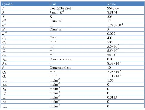
Table 1. Model parameters

Symbol Unit Value

F Coulombs mol-1 96485.4

R J mol-1K-1 8.3144

T K 303

km Ohm-1m-1 17

dm m 1.778×10-4

kaq Ohm-1m-1 5

dcell m 0.022

Ca Fm-2 400

Cc Fm-2 500

Va m3 5.5×10-5

Vc m3 5.5×10-5

Am m2 5×10-4

Yac Dimensionless 0.05

Kdec h-1 8.33×10-4

fx Dimensionless 10

Qa m3h-1 2.25×10-5

Qc m3h-1 1.11×10-3

in AC

C molm-3 1.56

in CO2

C molm-3 0

Xin molm-3 0

in H

C molm-3 0

2

in O

C molm-3 0.3125

in M

C molm-3 0

in OH

C molm-3 0

In order to overcome these shortcomings in conventional MPC, MPC with laguerre and exponential data weighting function are designed and compared for the two-chamber MFC. The z-transforms of the discrete-time laguerre networks have the following relationship [19-21]

  1  1 1

1

k k

z a

z z

az



 



  

 (18)

where a is the scaling factor, N is the number of terms, k is from 1 to N and 0 ≤ a < 1 for stability of the network. Let li(k) denote the inverse z-transform of i( , )z a , in which i is from 1 to N.

This set of discrete-time laguerre functions are expressed in a vector form as L(k)=[l1(k), l2(k),…,

lN(k)]T, and the laguerre sequences can be computed as:

( 1) ( )

L k HL k (19) in which

2

2 3

2 2 3 N-3 1 1

0 0 0 0 1

0 0 0

0 0

(0) 0

( 1)N N ( 1)N ( 1)N N

a

a a

a a a

H L

a a a a

a a a a



 



  

  

    

   

   _ 

   

    

 _    _ 

   

   

   

 _{ }   _ 

   

and 2

1 a

  . The expression of Laguerre function is a simple one which can make programming easier and reduce the calculating burdens; besides, it has a good effect on the parameterization, hence reduces the number of parameters required in modelling the control trajectory. At time ki, the control trajectory u k( ), i u k(i1), u k( i2),…u k( ik)… is regarded as the impulse response of a stable dynamic system. Thus, it can be approximated by a discrete polynomial function. Laguerre function is famous for its orthogonality, so u k( ) can be obtained by using Laguerre function.

What’s more, when the scaling factor is chosen at 0, the laguerre functions are equal to the expression of the traditional control variable, which is to say, Laguerre functions control strategy include the traditional MPC strategy. More precisely, at an arbitrary future sample instant k,

i j i j 1

( ) ( ) ( )

N

j

u k k c k l k



  



with ki being the initial time of the moving horizon window and k being the future sampling

instant. N is the number of terms used in the expansion, cj (j=1, 2, . . . , N) are the coefficients, and they

are functions of the initial time of the moving horizon window ki. Let [c c1 2 cN]T , and

T i

( ) ( )

u k k L k 

   can be obtained.

The traditional predictive formulation can be described as

P P P

P C

P P P

P

-1 -2

i P i i i i

-i

-1 -2

i P i i i i

-( ) ( ) ( ) ( 1

( 1)

( ) ( ) ( ) ( 1

N N N

N N

C

N N N

N N

x k N k A x k A B u k B u k

A B u k N

y k N k CA x k CA B u k CB u k

CA                      ） ） C i C ( 1)

B u k N 

(22)

After integrating Lagurge functions, they can be modified as

1

- -1 T 0

1

- -1 T 0

( ) ( ) ( ) , ( )

( ) ( )

m

m m i

i i i i i

i m

m m i

i i

x k m k A x k A BL i y k m k

CA x k CA BL i

           





where NP is the prediction horizon, NC is the control horizon, x k( im ki) and y k( im ki) are the

predicted state variables and the predicted output at ki + m with given current plant information x(ki).

Then a new expression of the cost function can be obtained

T T

2 ( )i

J     x k (24)

where T

L 1 ( ( ) ( ) ) P N m

m Q m R

    



 



1 1 T 0 ( ) ( ) m m i i

m A BL i

   







with _{QC C}T _.

To find the minimum of Eq. (24) without constraints, 1 _{is assumed existent. Then the optimal}

solution of the parameter vector η can be obtained by letting the partial derivative of the cost function approach to zero.

It is found that the condition number of the matrix  increases as the prediction horizon NP

increases. For a microbial fuel cell system, we assume that a=0.5, N=8, RL =0.1I. Here I is an unit

matrix. When NP is equal to 50, the condition number of the matrix  is 1.6748×107. When NP

increases to 100, the condition number increases to 2.4248×108, and when NP is 200, the condition

occur, and this numerical problem becomes severe when the plant model itself is unstable or when the dimension of the matrix A is large.

An exponentially weighted moving horizon window can convert the numerically ill-conditioned matrix  into a numerically well-conditioned in the presence of a large prediction horizon and could deal with great changes of the plant which originally get serious problems.

Define the sequence of exponentially weighted state variable and incremental control as

P

1 2 T

P

ˆ _{[ ( 1 ), ( 2 ), ,} j _{( ),} N _{( )]}

i i i i i i i i

X  x k  k  x k  k  x k j k  x k N k (25)

P

0 1

P

ˆ [ ( ), ( 1), , j ( ), N ( )]T

i i i i

U  u k  u k  u k j  u k N

         (26)

When  1, the weights decrease with the increase of sample j, thus the exponential weights de-emphasizes the state x(ki + j| ki) at the current time and less emphasis on those at future times. when

1

  , the situation just opposite, which de-emphasizes future times more than current time. As can be seen from Eq. (25) to Eq. (26), the key improvement is in that of the future states, and control variables are no longer have equal weights.

By using these exponentially weighted variables, the exponentially weighted cost function is expressed in terms of the transformed variables. The result is summarized as

P P

T T

1 0

ˆ N _{ˆ( ) ˆ( )} N _{ˆ( ) ˆ( )}

i i i i i L i

j j

J x k j k Qx k j k u k j R u k j

 







where Q and RLare weight matrices, x kˆ( _ij k_i) and u kˆ( _ij) are governed by the following

difference equation:

ˆ( _i 1 _i) Aˆ( _{i i}) B ˆ( _i )

x k j k x k j k u k j

 

       (28)

4. RESULTS AND DISCUSSION

In order to verify the control effect of these designed controllers, simulation operations of the MFC system with these controllers are carried out. For the purpose of designing MPC controller, Least Square Technique is used to identify the state space model of the microbial fuel cell described in the Section 2, and the identification solutions of the coefficient matrices are

 T  

d d d

0.9163 0.9972

, 0.4718 0.9163 , 133.757 0

0.8366 0.0055

A _ _ B  C 



  (29)

According to the principle of MPC, the parameter matrices corresponding to the basic increment-input-output model described in Eq. (16) can be derived as

 T  

122.5615 133.3825 1

0.9163 0.9972 0 , 3.1066 0.4718 0.91636 , = 1 0 0

0.8366 0.0055 0

A B C

 

 

_{ } 

 _ 

 

(30)

Hessian matrix, which is a square matrix of second partial derivatives of a scalar-valued function, often used to reflect the health status of a system. A system will be unhealthier when the Hessian matrix’s determinant is larger. The Hessian matrix for the microbial fuel cell system in this paper is + L

T

R

  . For the traditional model predictive control, when NP=20, NC=4, RL=0.8I, the

condition number of the Hessian matrix is 608140; when NP=50, the condition number of the Hessian

obvious that with the increase of the prediction horizon, the system performance getting worse and worse.

After amending the control algorithms with exponential data weighting functions, it is found that when a=0.5, N=10, RL=0.1I, =1.5, NP=50, the condition number of the Hessian matrix is 7550.

When NP=100, the condition number of the Hessian matrix is 7660.3 and when NP=200, the condition

number of the Hessian matrix is 7680.5. It is obvious that the system performance has been obtained a lot of improvement.

For a microbial fuel cell system, acetate concentration and temperature have great impacts on the output voltage. So, the feed flow rate of the cathode chamber and the anode chamber were selected as control variables and the influent acetate concentration and temperature as the disturbances, respectively. Three control strategies, including traditional MPC with reduced horizon control, improved MPC with Laguerre functions and improved MPC with exponential data weighting, are designed and compared in this paper.

When the plant is running under the traditional MPC, the predictive horizon is 20, the control horizon is 2, and the output weight is a unit matrix. When the plant is running under the MPC with laguerre functions substituting the control variables (LMPC) and under the exponentially weighted corrected MPC (EMPC), the two core factors are a is 0.3 and N is 4, the predictive horizon is 48, the weighting T

QC C, and RL=0.3I. What’s more,  is chosen as 1.5 in the MPC with exponentially

weighted corrected control strategy. The sampling time of the three control strategies is 1s.

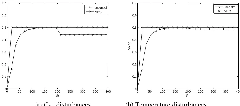
The output curves between the uncontrolled nonlinear system and those under MPC controller are compared first. Here, the operation status with the feed of the cathode chamber as input is simulated. The output voltage of the MFC is set at 0.5V, Qc is selected as the control variable. Two

kinds of disturbances are studied, one is that the concentrations of acetate CAC drops from 1.56molm-3

to 1.2molm-3 at the time of 200h, and the other is that the temperature reduces from 313K to 303K at the point of 200h. The output voltage curves for the traditional MPC (TMPC) controller and the original uncontrolled system are compared in Fig.1.

0 50 100 150 200 250 300 350 400 0

0.1 0.2 0.3 0.4 0.5 0.6 0.7

t/h

V

fc/

V

uncontrol MPC

0 50 100 150 200 250 300 350 400 0

0.1 0.2 0.3 0.4 0.5 0.6 0.7

t/h

V

fc/

V

uncontrol MPC

(a) CAC disturbances (b) Temperature disturbances

It can be seen from Fig. 1 that when there is no control action is applied, the MFC system needs a long time to get steady, and the output voltage has an obvious deviation from the setting value. However, when MPC is used to the system, the output voltage could follow the setting point in a short time, even though there exists a load disturbance.

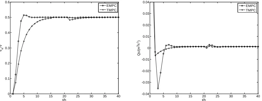
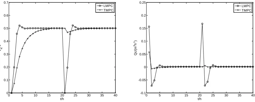
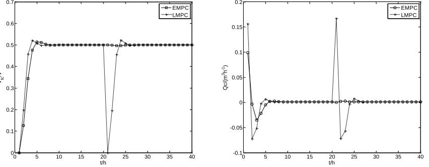
Simulation curves corresponding to temperature variation are shown in Fig. 2 to Fig. 4, the temperature drops from 313K to 303K at the time of 20h. The curves corresponding to acetate concentration changing are shown in Fig. 5 to Fig. 7, where CAC is reduced from 1.56molm-3 to

1.2molm-3 at 20h. In these figures, ‘TMPC’ stands for the traditional MPC strategy, ‘LMPC’ stands for improved strategy with Laguerre functions and ‘EMPC’ stands for the improved strategy with exponential data weighting.

Some phenomena can be observed from Fig. 2 to Fig. 7. Compared with general MPC, MPC with Laguerre functions make the MFC system present faster response and higher accuracy in stability. However, the overshoot and oscillation at perturbation point caused by MPC with Laguerre functions are more evident than that caused by general MPC.

0 5 10 15 20 25 30 35 40

0 0.1 0.2 0.3 0.4 0.5 0.6

t/h

Vfc

/V

LMPC TMPC

0 5 10 15 20 25 30 35 40

-0.1 -0.05 0 0.05 0.1 0.15 0.2

t/h

Q

c/

(m

3h -1)

LMPC TMPC

Figure 2. Comparison curves between TMPC and LMPC (T disturbances)

0 5 10 15 20 25 30 35 40

0 0.1 0.2 0.3 0.4 0.5 0.6

t/h

Vfc

/V

EMPC TMPC

0 5 10 15 20 25 30 35 40

-0.04 -0.03 -0.02 -0.01 0 0.01 0.02 0.03 0.04

t/h

Q

c/

(m

3h -1)

EMPC TMPC

0 5 10 15 20 25 30 35 40

0 0.1 0.2 0.3 0.4 0.5 0.6

t/h

Vfc

/V

EMPC LMPC

0 5 10 15 20 25 30 35 40

-0.1 -0.05 0 0.05 0.1 0.15 0.2

t/h

Q

c/

(m

3h -1)

EMPC LMPC

Figure 4. Comparison curves between LMPC and EMPC (T disturbances)

0 5 10 15 20 25 30 35 40

0 0.1 0.2 0.3 0.4 0.5 0.6 0.7

t/h

Vfc

/V

LMPC TMPC

0 5 10 15 20 25 30 35 40

-0.1 -0.05 0 0.05 0.1 0.15 0.2 0.25

t/h

Q

c/

(m

3h -1)

LMPC TMPC

Figure 5. Comparison between TMPC and LMPC (CAC disturbances)

However, MPC with exponential data weighting can make the MFC system present faster response, smaller overshoot and higher steady-state accuracy than general MPC, and it also can give more control effect than MPC with Laguerre functions.

By analysing of Fig.1 to Fig.7, we can also find some fact results. Both substrate concentration and environmental temperature are important factors that influence the operation performance of a microbial fuel cell. By real-time adjustment of the feed flow rate in cathode, the output voltage of the microbial fuel cell can be controlled at the given value even though it suffers from perturbations. Whether it is disturbance in substrate concentration or environmental temperature, the model predictive controller can resist the disturbance influence well.

can resist the influence of disturbances on the output voltage of MFC effectively. Further, the control scheme offered by this article is based on the advanced control technology, which is almost cannot be seen in references published so far. It is an effective way to improve the performance of microbial fuel cells by means of advanced control technology.

0 5 10 15 20 25 30 35 40

0 0.1 0.2 0.3 0.4 0.5 0.6 0.7

t/h

Vfc

/V

EMPC TMPC

0 5 10 15 20 25 30 35 40

-0.04 -0.03 -0.02 -0.01 0 0.01 0.02 0.03 0.04

t/h

Q

c/

(m

3h -1)

EMPC TMPC

Figure 6. Comparison curves between TMPC and EMPC (CAC as disturbances)

0 5 10 15 20 25 30 35 40

0 0.1 0.2 0.3 0.4 0.5 0.6 0.7

t/h

Vfc

/V

EMPC LMPC

0 5 10 15 20 25 30 35 40

-0.1 -0.05 0 0.05 0.1 0.15 0.2

t/h

Q

c/

(m

3h -1)

EMPC LMPC

Figure 7. Comparison curves between LMPC and EMPC (CAC as disturbances)

4. CONCLUSIONS

ACKNOWLEDGEMENTS

This work was supported by the Science and Technology special fund of Shenyang City under Grant F14-207-6-00, and the Science and Technology Research Project of Liaoning Education Department under Grant L2012140.

Reference

1. S. Das and N. Mangwani, J. Sci . Ind. Res. India, 69 (2010) 727. 2. B. E. Logan, Appl. Microbiol. Biot., 85 (2010) 1665.

3. J. Pukrushpan, A. Stefanopoulou and H. Peng, IEEE Contr. Syst. Mag. 24 (2004) 30.

4. C. Kunusch, P. F. Puleston, M. A. Mayosky and J. Riera, IEEE T. Contr. Syst. T., 17 (2009) 167. 5. S. Kaytakoglu and L. Akyalm, Int. J. Hydrogen Energ., 32 (2007) 4418.

6. A. Ashoori, B. Moshiri and A. K. Sedigh, J. Process Contr., 19 (2009) 1162. 7. L. F. Domınguez and E. N. Pistikopoulos, Ind. Eng. Chem. Res., 2 (2011) 609.

8. B. E. Logan, B. Hamelers, R. Rozendal, U. Schroder, J. Keller, S. Freguia, P. Aelterman, W. Verstraete And K. Rabaey, Environ. Sci. Technol., 40(2006) 5181.

9. X. Wang, J. Tang, J. Cui, Q. Liu, J. P. Giesy and M. Hecker, Int. J. Electrochem. Sci., 9 (2014) 3144.

10. A. Ashoori, B. Moshiri, A. K. Sedigh and M. R. Bakhtiari, J. Process Contr., 19 (2009) 1162. 11. J. H. Lee, Int. J. Control Autom., 9 (2011): 415-424.

12. C. Picioreanu, K. P. Katuri, I. M. Head, M. C. M. Loosdrecht and K. Scott, Water Sci. Technol., 57(2008) 965.

13. R. P. Pinto, B. Srinivasan, M. F. Manuel and B. Tartakovsky, Bioresource Technol., 101 (2010) 5256.

14. C. Picioreanu, I. M. Head, K. P. Katuri, M. C. Loosdrecht and K. Scott, Water Res., 41 (2007) 2921.

15. Kato M. A., C. I. Torres and B. E. Rittmann, Biotechnol Bioeng., 98 (2007) 1171. 16. Y. Zeng, Y. F. Choo, B. H. Kim and P. Wu, J. Power Sources, 195 (2010)79.

17. C. Picioreanu, M. C. Loosdrecht, T. P. Curtis and K. Scott, Bioelectrochemistry, 78 (2010)8 18. J. M. Correa, F. A. Farret, L. N. Canha, M. G. Simoes, IEEE T. Ind. Electron. 51 (2004) 1103. 19. L. Wang, J. Process Contr., 14 (2004) 133.

20. L. Wang, Model predictive control system Design and implementation using MATLAB, Springer, London (2009).

21. S. C. Patwardhan, S. Manuja, S. Narasimhan and S. L. Shah, J. Process Contr., 16 (2006):157-175. 22. X. Zhu, J. C. Tokash, Y. Hong and B. E. Logan, Bioelectrochemistry, 90 (2013): 30-35.

23. H. C. Boghania, J. R. Kim, R. M. Dinsdaleb, A. J. Guwyb and G. C. Premier, Bioresource Technol., 140 (2013): 277-285.