S ta b ility R e s u lts for F e e d b a c k C o n tro l
S y ste m s
A thesis submitted for the degree
of Doctor of Philosophy of
The Australian National University
W ynita May Griggs
2007
This thesis contains no material which has been accepted for the award of any other degree or diploma in any university. To the best of the author’s knowledge and belief, it contains no material previously published or written by another person, except where due reference is made in the text.
ABSTRACT
Several new stability results for system feedback interconnections are presented in this dissertation.
First, input-output stability results that capture a “blending” of the well-known small gain and passivity theorems, are provided. In the frequency domain, a system assumption of “small gain” over certain frequency intervals (as opposed to the entire frequency range) and “passivity” over the remaining frequency intervals (as opposed to the entire frequency range), is placed on each of two, stable, linear time-invariant (LTI) systems in a feedback interconnection. It is shown that input-output stability of the feedback interconnection follows. The frequency-dependent system assump tion and associated input-output stability result are obtained by using a notion of dissipativity.
A “mixed” small gain and passivity assumption is then defined for causal, non linear systems in the time domain. An associated input-output feedback stability result is observed by placing a bound on the feedback system error and output sig nals in terms of bounded input signals.
sta-Abstract
bility robustness condition presented in this dissertation provides a single constraint on a controller (in terms of the generalized robust stability margin) such that all
plants in the uncertainty set are (sufficiently guaranteed to be) stable.
ACKNOWLEDGEMENTS
I would like to express my sincere appreciation to Dr. Alexander Lanzon (formally of the Department of Information Engineering, Research School of Information Sci ences and Engineering (RSISE), The Australian National University (ANU); and National ICT Australia (NICTA)), and to Prof. Brian Anderson (of the Depart ment of Information Engineering, RSISE, ANU; and NICTA), for supervising my progress during the four years of my PhD candidature. Their knowledge and guid ance has been invaluable. I would also like to thank Dr. Michael Rotkowitz, who recently joined the Department of Information Engineering, for his contribution to my supervision during the final few months. 1 am grateful to Prof. Matthew James (of the Faculty of Engineering and Information Technology), and to Prof. David Hill and all of the other academic staff of the Department of Information Engineering with whom I have had discussions of a technical nature.
I would also like to thank the general staff of the ANU College of Engineering and Computer Science for their help with m atters of an administrative or IT nature - especially Mrs Rosemary Shepherd and Mrs Lesley Goldburg, Mrs Debbie Pioch and Ms Suzanne Van Haeften, and Mr James Ashton and Mr Peter Shevchenko. Thanks to Miss Lilangie Perera who, during her summer scholar experience at the Department of Information Engineering, wrote the Matlab code for the example given in Section 5.6 of this dissertation.
CONTENTS
A b s tr a c t... i
A cknow ledgem ents... iii
Table o f C o n ten ts... v
Notation and A c r o n y m s...vii
1. Introduction... 1
1.1 B ac k g ro u n d ... 1
1.2 Aim and M o tiv atio n s... 4
1.2.1 Problem 1: “Mixed” small gain and passivity properties . . . . 4
1.2.2 Problem 2: Linear time-varying uncertain sy ste m s... 7
1.3 Organization of the D issertatio n ... 10
2. Basic Stability R e s u l t s... 11
2.1 Input-output Stability R e s u lts ... 11
2.2 The LTI i'-gap Metric and Associated Stability R e s u lts ... 13
2.2.1 Generalized Robust Stability M a r g i n ... 14
2.2.2 The LTI i'-gap Metric ... 14
2.2.3 Stability Results ...14
3. A “M ixed” Property for Linear Time-invariant S y s te m s... 17
3.1 In tro d u ctio n ... 17
3.2 System Descriptions ...20
3.3 The Feedback In terco n n ectio n ... 25
3.4 Main Stability T h e o r e m ... 27
3.5 C o n clu sio n s... 32
4. Nonlinear Systems with “M ixed” P r o p e r tie s... 33
4.1 In tro d u ctio n ... 33
4.2 Feedback System Description ... 37
4.3 The “Mixed” Small Gain and Passivity P ro p erty ... 38
vi Contents
4.5 C o n clu sio n s...45
5. The Structured L T V Uncertainty Stability P r o b le m... 47
5.1 In tro d u ctio n ... 47
5.2 The Scaled Small Gain C o n d itio n ...50
5.3 The Scaled LTI iz-gap Metric C ondition... 53
5.4 A LMI Feasibility P ro b le m ... 56
5.5 Solution A lg o rith m ... 64
5.6 Numerical E x a m p le ... 66
5.7 C o n clu sio n s... 70
6. A Special Case o f the Scaled LTI v-gap Metric C on d itio n... 71
6.1 In tro d u ctio n ... 71
6.2 Problem S e t - u p ...72
6.3 A “Worst-case” LTI iz-gap M e tr ic ... 74
6.4 The Stability Robustness C o n d itio n ... 77
6.5 C o n clu sio n s... 78
7. Concluding C o m m e n ts...81
7.1 C o n clu sio n s... 81
7.2 Future D ire c tio n s...82
Appendix' 85 A. The Induced R ea liza tio n... 87
A.l Induced Realizations for L F T s ...87
A.2 Internal S t a b i l i t y ... 91
A.3 Linear Time-Varying Internal S ta b i l i t y ... 93
B. Apt + Bf1Ff1 is H u r w i t z... 97
NOTATION AND ACRONYMS
R real n u m b e rs
R + n o n -n e g a tiv e real n u m b e rs
C co m p lex n u m b e rs
(^ynxri m a tr ix of com plex n u m b e rs w ith m row s a n d n colu m n s j th e im a g in a ry u n it, ie: j = y / —l
R e ( s) real p a r t of s G C
a co m p lex c o n ju g a te of a co m p lex n u m b e r a
3 th e re ex ists
V for all
su ch t h a t
G belongs to
:= defined by
□ en d of p ro o f
< less th a n
< less th a n or eq u a l to
> g re a te r th a n
> g re a te r t h a n or eq u al to
< n o t less th a n
-> m ap s to; te n d s to
=> im plies
is im p lied by is e q u iv a len t to
x G ( a , 6) a < x < b w h ere a, x, b G R x G ( a , 6] a < x < b w h ere a, x, b G R x G [a , 6) a < x < b w h e re a, x, b G R x G [a , b] a < x < b w h ere a, x, b G R m in{ } m im im u m e le m en t of a se t m ax { } m a x im u m ele m en t of a se t
lim x^ a f ( x ) lim it of th e fu n c tio n f ( x ) a s x te n d s to a in f X€x f ( x ) in fim u m of th e fu n c tio n f ( x ) over x G X SUPxGA- f ( x ) s u p re m u m o f th e fu n c tio n f ( x ) over x G X
1 • 1 a b s o lu te value; n o rm
viii Notation and Acronyms
0 z e r o o p e r a t o r
/ i d e n t i t y m a t r i x o f c o m p a t i b l e d im e n s i o n s ; i d e n t i t y o p e r a t o r
I n i d e n t i t y m a t r i x o f d i m e n s i o n n x n [a ij\ i jt h e l e m e n t o f m a t r i x A
A T t r a n s p o s e o f m a t r i x A A - 1 in v e r s e o f m a t r i x A d e t ( A ) d e t e r m i n a n t o f m a t r i x A
d i a g ( A i , . . . , A n ) b lo c k d i a g o n a l m a t r i x o r o p e r a t o r
Fu( A , B) u p p e r l i n e a r f r a c t i o n a l t r a n s f o r m a t i o n o f m a t r i c e s A a n d B Fi( A , B ) lo w e r l i n e a r f r a c t i o n a l t r a n s f o r m a t i o n o f m a t r i c e s A a n d B A * B R e d h e f f e r s t a r - p r o d u c t
£ P( R ) , C P{ R + ) s p a c e o f f u n c t i o n s { / : R —► R } s u c h t h a t t —> \ f ( t ) \ p is i n t e g r a b l e o v e r R , R + r e s p e c t i v e l y ; t y p i c a l l y p = 1, 2, o o
c2( M ) f r e q u e n c y d o m a i n H i l b e r t s p a c e o f s q u a r e i n t e g r a b l e
f u n c t i o n s o n jR i n c l u d i n g o o
n
2 s u b s p a c e o f C 2(jWi) w i t h f u n c t i o n s a n a l y t i c in R e ( s) > 0 (ie: o p e n r i g h t - h a l f p l a n e )F o c i M ) f r e q u e n c y d o m a i n B a n a c h s p a c e o f f u n c t i o n s t h a t a r e
( e s s e n t ia l ly ) b o u n d e d o n jR i n c l u d i n g o o
H oo s u b s p a c e o f / ^ ( j R ) w i t h f u n c t i o n s t h a t a r e a n a l y t i c a n d b o u n d e d in R e ( s ) > 0
n
s e t o f p r o p e r r e a l r a t i o n a l t r a n s f e r f u n c t i o n m a t r i c e s'j^rnxn s e t o f p r o p e r r e a l r a t i o n a l t r a n s f e r f u n c t i o n m a t r i c e s w i t h m ro w s a n d n c o l u m n s
p r e f ix 7Z s u b s p a c e o f r e a l r a t i o n a l f u n c ti o n s , eg: VSHoo
X p r o d u c t d o m a i n
I Q C i n t e g r a l q u a d r a t i c c o n s t r a i n t L F T l i n e a r f r a c t i o n a l t r a n s f o r m a t i o n L H S l e f t - h a n d s id e
L M I l i n e a r m a t r i x i n e q u a l i t y L T I l i n e a r t i m e - i n v a r i a n t L T V l i n e a r t i m e - v a r y i n g M I M O m u l t i - i n p u t , m u l t i - o u t p u t R H P r i g h t - h a l f p l a n e
R H S r i g h t - h a n d s id e
1. INTRODUCTION
1.1 Background
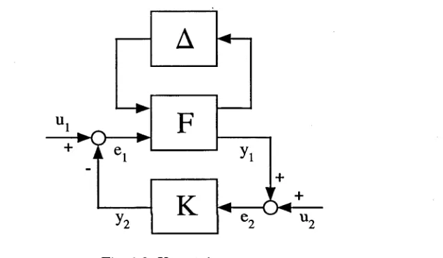
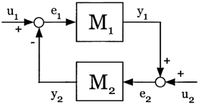
Stability results for feedback control systems are provided in this dissertation. Feed back is a basic concept of control theory. O utput variables of a system to be con trolled are measured, and this information is processed to generate an input to the system to be controlled such th at the overall set-up behaves in some desired fashion. A model applicable to most feedback systems is shown in Fig. 1.1. Here, U\ and U2 denote (external) input signals, e\ and denote error signals, and y\ and y2 are output signals. The notation K is associated with the controller and the notation P is associated with the system to be controlled. The feedback control system pictured in Fig. 1.1 is referred to as a negative feedback control system.
Fig. 1.1: Feedback control system.
Feedback is used for a number of reasons. One of these is to reduce the effect of any unmeasured disturbances acting on the system [86]. Another is to reduce the effect of any uncertainty about the system dynamics [86]. That is, an aim of using feedback is to minimize the effects of lack of knowledge about a system which is to be controlled. In the absence of uncertainty then, there may be no need for feedback, and decisions could be made “open-loop” [95]. However, systems (plants, sensors or actuators) are not free of uncertainty [95].
Feed-2 1. Introduction
back system well-posedness is essential as it relates to whether a mathematical model is adequate as a description of a physical system. More accurately, it corresponds to a question of existence and uniqueness of solutions to the equations
which describe the feedback system shown in Fig. 1.1, together with the equations
(That is, it corresponds to a question of existence and uniqueness of solutions for , ^2, 2/i, 2/2 for each choice of u i , u 2) [6,39,84,85,95]. It is usual in the defini
tion of well-posedness to further require that the errors and the outputs depend on the inputs in a non-anticipatory way; and that the errors and the outputs depend, on finite intervals, Lipschitz continuously on the inputs. (Lipschitz continuity is a smoothing condition for functions that is stronger than regular continuity. In tuitively, a Lipschitz continuous function is limited in how fast it can change: a line joining any two points on the graph of this function will never have a slope steeper than a certain number called a Lipschitz constant of the function.) Ref erences [6, 39, 84, 85, 95] provide conditions to impose on P and K to guarantee well-posedness of the feedback-loop. Well-posedness is not discussed in detail in this dissertation; it is assumed of most feedback interconnections under consideration.
Stability is a desired property of a feedback control system. The study of sys tem stability has a rich history and there are many different notions of stability of systems. In all cases, the idea of determining stability involves determining whether a system is well-behaved in some sense, given a set of system equations.
The different notions of stability are often based on the way a physical system is mathematically described. Two important ways of mathematically describing phys ical systems are as follows. The first way is to give an internal description of the physical system. This approach uses the physical laws and internal interconnections governing the system as the basis of the mathematical model. Accordingly, this description generally takes the form of an ordinary differential equation or a partial differential equation. Also, one works with a set of intermediate variables (related to the concept of state). As a result, there are two parts to mathematical models that internally describe systems: a dynamical part, which describes the evolution of the state under the influence of the inputs; and a memoryless part, which relates the output to the state (and sometimes to the instantaneous value of the input as
e i = ui — y2
e2 = u2 + y\
(1.1)
(1.2)
1.1. Background 3
well).
Stability, in relation to the internal (or state-space) description of a system, is regarded as an internal property. The system is considered as excited by an initial condition, and boundedness or convergence of the state for future time is taken as the basic stability requirement. In other words, stability in the state-space descrip tion sense is concerned with the behavior of trajectories of a system when its initial state is near equilibrium; the object is thus to draw conclusions about the behav ior of a system without actually focusing on particular solution trajectories. From a practical viewpoint, stability in this sense is im portant because external distur bances such as noise, wind and component errors are always present in a real system to perturb it from equilibrium.
One of the founders of stability theory in the internal description sense was the Russian mathematician A. M. Lyapunov [62]. He introduced many of the basic definitions of stability th at are in use today, and also proved many of the fundamental theorems. Some extraordinary contributions to the field were made by V. A. Yakubovich, V. M. Popov and R. E. Kalman (see [55, 74, 97] for exam ple). Modern systems theory relies heavily on the state formulation for synthesis techniques, as illustrated by some of the highlights of modern control theory: for example, Pontryagin’s maximum principle [73]; the regulator problem for linear sys tems [57]; and the Kalman-Bucy filtering theory [56,58].
The input-output approach is the second way to mathematically describe a phys ical system. Here, the mathematical model usually takes the form of an operator equation expressing the relationship between the inputs (the variables to be ma nipulated) and the outputs (the variables of interest). Such a description is often obtained from some representative experiments. Significantly, the input-output ap proach relates external variables: the system is viewed as a “black box” and the description does not depend in any way on the notion of state. In other words, this approach requires minimal knowledge of the physical laws governing the system and of the interconnections within the “black box” . The input-output description provides the benefits of abstraction: because it is free of details about the internal description, basic results in system theory can be viewed more easily. In system design, this approach facilitates designing for a prescribed response to a specified class of inputs.
4 1. Introduction
of the output in terms of the norm of the input.) The successful development of input-output stability theory occurred much more recently than the development of Lyapunov theory. It was pioneered by I. W. Sandberg [79] and G. Zanies [100,101] in the 1960’s.
Relationships between the internal and input-output notions of stability exist: J. C. Willems, for example, illuminated some of these relationships in [91] (the input-output and state space representations of systems are not interchangeable, however [99]). For instance, the circle criterion, Popov criterion, passivity theorem and small gain theorem are a few of the important stability results obtained over the last few decades. These results have counterparts in each of the internal and the input-output approaches (although the abstract results on passivity and system gain emerged via input-output methods; for example, see [102,103]).
1.2 Aim and Motivations
The aim of this dissertation is to propose several stability results for feedback system interconnections, and in so doing, expand on the feedback control system stability theory available. Two distinct stability problems are addressed. The first is posed and solved based on the input-output systems theory approach. Internal, or state- space, system descriptions are considered in the second problem. A brief description of each of the two problems is provided below, with motivation for their study, and summaries of some of the key techniques used in this dissertation to solve them. A review of some of the key methods used in the literature to solve similar problems is also provided where appropriate.
1.2.1 Problem 1: “M ixed” small gain and passivity properties
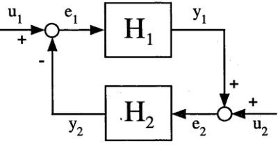
The first problem involves determining input-output stability of a negative feedback interconnection as shown in Fig. 1.1 (or as shown below in Fig. 1.2). The abstract reasoning of the input-output approach has lead to the development of some very important stability theorems such as the small gain theorem [100, 101] and the passivity theorem [15,78,100,101]. It is possible to set up a general input-output framework which supports results such as these. Consider the negative feedback interconnection shown in Fig. 1.2. The input, error and output signals are functions of time, defined for t > 0; and they take values in some (real-valued) normed space. Recall that two of the four equations describing the feedback system shown in Fig. 1.2 were given by (1.1) and (1.2). The symbols M\ and M2 are operators acting on their respective inputs e\ and e2 to produce outputs y\ and 2/2, respectively. Then the input-output stability problem is to show that if U\, 112 belong to some class of
1.2. Aim and Motivations 5
class of functions.
Fig. 1.2: Negative feedback interconnection.
Typically, input-output stability results are obtained by assuming th at systems have specific properties associated with them. For instance, the small gain theorem ensures stability provided that the product of the gains of the two systems in the feedback interconnection is less than one. The passivity theorem guarantees stabil ity, for example, if both systems in the feedback interconnection are passive, and one of them is input strictly passive with finite gain. Of course, there exist many situations where stability cannot be determined by use of the small gain or passivity theorems because the assumptions required on systems as stated in the theorems do not appropriately match the properties of the actual systems in the feedback inter connection in question. In this dissertation, small gain and passivity properties are
“blended” in an appropriate way as to create a (super) class of system assumptions (which captures systems described by small gain concepts and passivity concepts). Input-output stability results of feedback interconnections are consequently derived.
Obtaining such results has practical applicability. For instance, it has been ob served that high frequency dynamics can frequently destroy the passivity property of an otherwise passive system. A celebrated controversy in adaptive control [77] depended on the observation th at passivity conditions, normally forming part of the hypotheses used in the proofs of convergence of certain adaptive control algorithms, should not be assumed to be valid in practice (because high frequency dynamics of ten neglected for modelling purposes will always be present in a real system). Failure of the passivity condition invalidated the applicability of the associated theorem on the algorithm convergence to most real-life applications, and left a cloud hanging over the real-life use of the algorithm. Simulations of [77] confirmed that adverse be havior could occur when high frequency dynamics were explicitly taken into account.
6 1. Introduction
adaptive systems of the type examined in [77]; that is, where “passivity” properties hold only for low frequency signals. Stability is established if additionally (and in a rough manner of speaking), “gains” are small at high frequencies (ie: a small gain property in the sense of the small gain theorem holds in the frequency band where the passivity condition fails). Thus, an important class of applications in which passivity and small gain ideas have to be “blended” has been illustrated.
Extensions to stability-associated results to accommodate system properties in specific frequency bands have recently been developed. For example, [51] extended the “static” concept of dissipativity to a “dynamic” , frequency-dependent frame work for linear time-invariant (LTI) systems.
Dissipativeness is a property, presented in this thesis as an input-output property of a general dynamical system, which captures concepts such as passivity and finite gain. The study of dissipative systems was initiated by J. C. Willems [93] in order to tie together ideas common to network theory and feedback control theory, as well as thermodynamics and mechanics. (Beyond the dissipative systems theory associ ated with network synthesis of the 1930s, this work can be seen as evolving from a series of studies, beginning with the Kalman-Yakubovich lemma [55, 96] and its applications [5,7,22,94], which can be interpreted as exploring the usefulness of the concept of passivity or positive real transfer functions.) In [93], dissipativeness was defined as essentially a generalization of the property of passivity via an inequality based on a state-space description. In other words, dissipativeness was introduced as a concept which reflected something of the internal properties of the system.
1.2. Aim and Motivations 7
The paper [47] provides another example of where extensions to stability as sociated results to accommodate for system properties in specific frequency bands have been developed. The paper [47] generalized the Kalman-Yakubovich-Popov lemma to establish a relationship between a frequency domain inequality in a fi nite frequency range, and a linear matrix inequality (LMI) condition. (The stan dard Kalman-Yakubovich-Popov lemma treats frequency domain inequalities, which characterize various properties of dynamical systems, for the entire frequency range only.) See also [48-50,81,98] for results regarding restricted frequency ranges.
On another note, the use of integral quadratic constraints (IQCs) to describe systems in feedback interconnections was introduced in [67] as a powerful method of determining closed-loop stability. The result assumes that one of the systems in the feedback interconnection is described by a LTI operator, while the other system represents the “trouble-making” (nonlinear, time-varying or uncertain) components of the feedback loop. The stability theorem [67, Theorem 1] then captures the clas sical small gain and passivity/dissipativity theorems under the proviso th at one of the two cascaded systems in the loop is LTI.
The “blended” small gain and passivity properties described in this thesis are referred to as “mixed” small gain and passivity properties. In the first instance (mo tivated by a desire to accommodate for frequency range specific systems properties), a LTI “mixed” small gain and passivity frequency domain property is defined using the notion of dissipativity. It is shown th at (finite-gain, and hence) input-output stability of a feedback interconnection consisting of two multi-input, multi-output (MIMO) LTI systems with “mixed” small gain and passivity frequency domain prop erties is guaranteed. The interconnected dissipative systems approach (as opposed to an IQC approach, which would seem readily possible) is used, as the methodology paves the way for a similar result when the systems are nonlinear. Consequently, a “mixed” small gain and passivity time domain property is defined for nonlinear systems, and it is shown that input-output stability of a feedback interconnection consisting of two nonlinear systems with these “mixed” properties is certain.
1.2.2 Problem 2: Linear time-varying uncertain systems
uncertain-8 1. Introduction
ties, or when the plant contains a number of uncertain parameters.
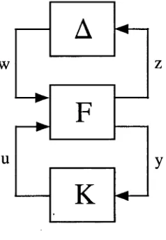
The second problem addressed in this dissertation involves determining internal stability of a system subject to bounded linear time-varying (LTV) uncertainties, given that a nominal feedback interconnection, consisting of a LTI system P and a LTI controller K as shown in Fig. 1.1, is internally stable. Often it is suitable to describe such a problem using a linear fractional transformation (LFT) framework, as shown in Fig. 1.3, where F(s) is a transfer function matrix th at describes the relationship between the nominal LTI plant P and the structured LTV uncertainty denoted by A.
Fig. 1.3: U ncertain system .
This type of stability problem has been studied intensively in the literature. For instance, [8] reduced the problem (where A was possibly nonlinear) to a question of existence of a quadratic Lyapunov function of a certain structure. The existence of the Lyapunov function was determined by solving a convex optimization prob lem. In [71], where complex-valued uncertainty was considered, quadratic stability (which is related to the existence of quadratic Lyapunov functions) was shown to be equivalent to a scaled H ^ norm condition when the structured uncertainty consisted of only two diagonal blocks. (The equivalence for more than two blocks is not in general true [71].)
[image:17.529.131.449.284.469.2]1.2. Aim and Motivations 9
The paper [66] considered structured slowly time-varying uncertain gains and ob tained a sufficient frequency domain condition for stability when pairs of the un certain gain and its derivative belonged to a given convex set. A sufficient stability condition (that could be formulated in terms of LMIs) was derived in [9], and was shown to be less conservative than a standard scaled small gain stability condition when the uncertainty structure contained real, repeated, time-varying parameters (ie: when sub-blocks of the uncertainty structure shared the same scalars). Obtain ing this condition did not require the use of IQCs [54], or the explicit construction of a quadratic Lyapunov function [71]; but followed from basic properties of the struc tured singular value (although the results are closely related to notions of quadratic stability - [71] used the quadratic stability approach to derive the condition for the case where all of the parameters are complex).
In [83], a computational approach was developed for designing a globally optimal controller th at was robust to time-varying nonlinear perturbations in the plant. The controller design problem was formulated as an optimization with bilinear matrix inequality constraints, and solved to optimality by a branch-and-bound algorithm (see [24] for instance). A branch-and-bound scheme was also used in [59] to obtain a globally optimal solution to a robust synthesis problem.
The main contribution of this thesis in regards to the stability robustness prob lem shown in Fig. 1.3 (where A is structured LTV uncertainty, and F and K are LTI) concerns the development of a sufficient scaled LT1 lz-gap metric stability ro bustness condition. This scaled LTI zz-gap metric condition is an extension of a standard, necessary and sufficient, scaled small gain condition (which is described in [17,20,80]). An advantage of the scaled LTI zz-gap metric condition is that, apart from a comparison with a generalized robust stability margin as the final part of the stability test, the solution algorithm implemented to test the condition is indepen dent of the controller.
10 1. Introduction
the z/-gap metric [3,87,88] exist. Analytical computations of the metrics in these cases are generally not possible.
1.3 Organization of the Dissertation
2. BASIC STABILITY RESULTS
This chapter presents important stability results and associated mathematical pre liminaries from the literature th at are relevant to this thesis.
2.1 Input-output Stability Results
A desired property of a feedback interconnection of two systems is th at the inter connection is input-output stable [95]. To determine stability, one typically places assumptions on the two systems in the interconnection; and shows that, if the closed- loop system’s inputs belong to some class of functions (such as the Cp spaces), then the errors and outputs also belong to the same class of functions [19]. To illustrate, a negative feedback interconnection is shown in Fig. 4.1, where H \ and H2 are operators acting on the errors e\ and e2, respectively, to produce outputs y\ and y2, respectively.
Fig. 2.1: Input-output stability framework.
[image:20.529.169.369.438.543.2]12 2. Basic Stability Results
“mixed” small gain and passivity properties, discussed later in this thesis.)
We select our working signal space to be the £ 2-space in particular (although fre quently the £p-spaces in general are considered). Recall that £ 2[0, oo) is a Lebesgue space with inner product defined as
where the superscript (•)' denotes the vector transpose. The norm of functions in £ 2[0,oo) is denoted by || • ||, where | | / | | 2 := ( / , / ) . For T G [0, oo), Py denotes the truncation operator. That is, for a function /(£), 0 < t < oo,
For convenience, the notation f r := P r f is used. Then £ 2e denotes the extension of the space £ 2[0, oo), defined by C2e := { / : f c G £ 2[0, oo) VT G [0, oo)}.
D efinition 1. [64, Definition 6.5] A system, or more precisely, the mathematical representation of a physical system, is defined to be a mapping H : £ 2e —> £ 2e, that satisfies the so-called causality condition
D efinition 2. [64, Definition 6.6] A system H : £ 2e —> £ 2e is said to be input-output
C2~stable if, whenever the input belongs to £ 2[0, oo), the output is once again in
£ 2[0, oo) (ie: H is input-output C2~stable if H f G £ 2[0, oo) whenever f G £ 2[0, oo)).
For simplicity, input-output £ 2-stability will be referred to as input-output sta bility, or simply stability, when the context is clear.
Theorem 1. (Sm all Gain T heorem ) [19] Consider the feedback interconnection
shown in Fig. 2.1. Let H\, / f 2 : £ 2e —> C2e• Let e i,e 2 G £ 2e and define U\ and u2 by
(Hf('))r =
(Hf T(‘))T
for all f G £ 2e and all T G [0, oo).
U\ — e\ + / / 2e2
u 2 — e 2 — H \ e \ .
Suppose that there are constants 771,772, e\ > 0, e2 > 0 such that
\\(H\ei)T\\ < eilleirll +771
2.2. The LTI v-gap Metric and Associated Stability Results 13
VT G [0, oo). Under these conditions, if e\e2 < l, then
II^ItII ^ (1 — ^162) 1 (II^fclT’ll + e211^27"II + ^2 + e2rh) (2-1)
||e2r|| < (1 - €i€2)~1 (||w2t|| + €i||uit|| + 771 + e ^ ) (2.2)
VT G [0,00). Furthermore, if ||wi||, ||u2|| < 00 then e i,e 2 and 2 / 1, y2 have finite norms, and the norms of the errors are bounded by the right hand sides of (2.1) and (2.2), provided all subscripts T are dropped.
Proof of the small gain theorem is provided in [19]. Before proceeding with a statement of the passivity theorem, we define ( f , g ) r ' = (fr^gr) and note that
{ f r , gr ) = ( f r , g) = (f,
9r)-Theorem 2. (P assivity 9r)-Theorem ) [19] Consider a feedback system as shown in Fig. 2.1 and described by
e\ — U\ — H2e2
e2 = u2 + t f j f i i
where Hi, H 2 : C2e —* C2e- Assume that for any u \,u 2 G £ 2[0, 00), there are solu tions e i,e 2 G T2e- Suppose that there are constants e\, ip, li, f)\, k2, f)2 such that
|I(#i/ )t|| < eill/rll + Vi
(.f,H J )T >h\\fT\\2 + fh
( W U ) T > h \ \ ( H 2 f ) T \ ? + fh
V / G C2e, VT G [0,oo). Under these conditions, if
l\ k2 ~> 0 (2.3)
then U\,U2 G >C2[0, 00) imply that e\, e2, H \e\, H2e2 G T 2[0, 00).
For a proof, see [19].
Rem ark 1. When k2 — 0, (2.3) requires that 11 > 0; then the theorem holds if H\ is input strictly passive with finite gain and H2 is passive.
The notions of passivity, input strict passivity and finite gain are formally defined in Chapter 4.
2.2 The LTI is-gap Metric and Associated Stability Results
14 2. Basic Stability Results
2.2.1 Generalized Robust Stability Margin
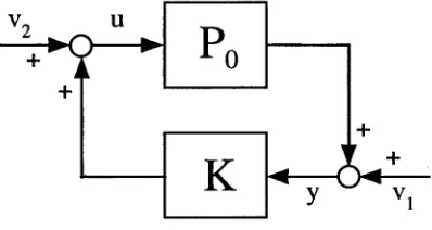
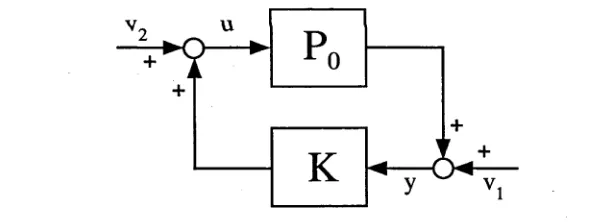
Let a feedback interconnection consisting of a nominal LTI plant Pq and a LTI controller K, as shown in Fig. 2.2, be denoted by [Pq,K ]. This interconnection is said to be internally stable if it is well-posed and each of the four transfer functions mapping the signals v\ and to y and u are stable; that is, they belong to TTHoo [104, Lemma 5.3]. The generalized robust stability margin bp0iK [30,75,86] is given by
b p 0 , K := p o ) ( / - K P 0)~l ( I K )
if [P0. K] is internally stable; and by 5p0,x := 0 otherwise. It is also possible to define bopt(Po) supK bp0tx [86]. It is shown in [30] th at bopt(Po) < 1 for any Pq.
+ < > — ►
Fig. 2.2: Internal stability of [Pq,K \.
2.2.2 The LTI v-gap Metric
A convenient formulation of the i'-gap metric, 6„(Po,Pi), between two systems P0,P i G 7Znxm, is given by: 6u(P0j P\) := H G i G o l l o o if
det(GlGo)(ju)
7^ 0 Vo; G(—00,00) and wno(det(G’jGro)) = 0; and by 6l/(P0, Pi) := 1 otherwise [86,90]. Here
Gi,Gi denote normalized right and left graph symbols, respectively, for plants P;,
i = 0,1 (where an account of normalized right and left graph symbols is given in [86]); and wno(g) denotes the winding number about the origin of g(s) (or num ber of encirclements of the origin made by p(s)), as s follows the standard Nyquist D-contour (see [86, Section 1.2.2] for more details). An efficient state-space method for computing 6„(P0j P\) is provided in [86, Appendix A.2].
2.2.3 Stability Results
[image:23.529.164.363.313.419.2]2.2. The LTI v-gap Metric and Associated Stability Results 15
bp^K > bp0^K ~ öu(Po, Pi); (2.4)
and by the stronger inequality
arcsin bpx_p > arcsin bp0_x — arcsin<5„(Po, Pi)
(the second inequality implies the first) [86,90]. Inequality (2.4) demonstrates that a feedback interconnection [Pi, K] is internally stable provided (the feedback inter connection [P0,K] is internally stable, and) 5v{Pq,P \) is strictly less than bp0tg. In fact, for a given controller K th at achieves bp0tx (where bp0^ > ß > 0), the set {P : öu(Pq, P) < ß] is a neighborhood or “ball” of systems about P0 that are guar anteed to achieve a generalized robust stability margin of at least bp0 ^ — ß with K .
These points correlate with part (i) of the following lemma.
Lem m a 1. [86, Remark 3.11]
(i) Given a nominal plant Po E 1Znxm, a controller K € 7£mxn and some number
ß E (0,6opt(P0)), then [P\,K] is internally stable for all plants P\ E R,nxm satisfying 6U(P0, Pi) < ß if and only ifbp0j< >
ß-(ii) Given a nominal plant Po E lZnxrn, a perturbed plant P\ E 7Znxm and a positive
number ß < b^ßPo), then [Pi,K] is internally stable for all controllers K E
JZmxn satisfying bp0^ > ß if and only if Ö„(P0, Pi) < ß.
Part (ii) of the above lemma states that any plant at a distance greater than ß
3. A “MIXED” SMALL GAIN AND PASSIVITY FREQUENCY
DOMAIN PROPERTY FOR LTI SYSTEMS1
3.1 Introduction
Two of the most important results in the input-output stability theory of intercon nected systems are the small gain and passivity theorems. The small gain theorem states th at if the product of the gains of two stable systems is less than one then the feedback interconnection of the two systems is stable [19,32,64,104] (see Theorem 1). The passivity theorem guarantees stability of a feedback interconnection of two stable systems if, for instance, both of the systems are passive, and one of them is input strictly passive with finite gain [19,32,64,82] (see Theorem 2). Of course, there exist many situations where stability of an interconnection cannot be guaran teed by use of the small gain or passivity theorems alone because the properties of the systems in the feedback-loop in question are not compatible. One instance is the adaptive control example given in Section 1.2.1.
The idea of merging the passivity and small gain theorems to provide stability results for feedback interconnections containing systems belonging to a class that encompasses those dealt with by the small gain theorem and passivity theorems alone, would therefore be extremely useful. For example, consider two open-loop, causal, stable, single-input single-output (SISO) systems with LTI transfer functions, say
m i(s) = (s + l)(s + 2)
and
ma(s) = (s + 3)(s + 4)
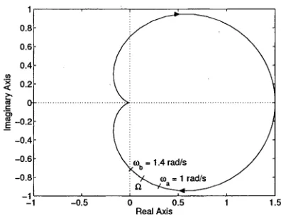
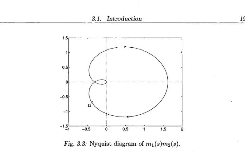
with Nyquist diagrams shown in Figs. 3.1 and 3.2. It is clear that, if in some frequency range [0, Q] the systems are passive (ie: the real part of each of the transfer functions is positive), and if in the frequency range [$2, oo) the product of the amplitudes of the transfer functions is less than one, then there is no way that
18 3. A “Mixed” Property for Linear Time-invariant Systems
the Nyquist diagram of the cascade would encircle the point —1 + j0. Accordingly, the closed-loop would be stable. (Indeed, as depicted in Figs. 3.1 and 3.2, such an Q
exists, and the Nyquist diagram of mi(s)rri2(s) shown in Fig. 3.3 does not encircle
- 1 + j O . )
= 1.4 rad/s = 1 rad/s
Real Axis
Fig. 3.1: Nyquist diagram of m i(s).
= 1 rad/s = 1.4 rad/s
Real Axis
Fig. 3.2: Nyquist diagram of m2(s).
Obviously, however, m i(s) and rri2(s) are not of a form that allows treatm ent
of closed-loop stability by the small gain or passivity theorems. Furthermore, one could not simply scale one of the systems with transfer functions rai(s) or rri2(s)
[image:26.529.162.360.206.358.2]3.1. Introduction 19
Fig. 3.3: Nyquist diagram of mi (5)7722(s).
result in an increase to the other system’s gain. T hat is, absolute feedback-loop gain is constant. Similarly, multipliers (or weights) cannot always be used to transform a feedback-loop such that the passivity theorem can be applied. There do exist transformations in the literature th a t transform a passive system to a system with gain less than one; and vice versa [19,64], Using this idea, one could consider finding (frequency-dependent) transformations that transform “mixed” small gain and pas sive systems (as illustrated by systems with transfer functions m i(s) and m 2(s)) into either systems with small gain properties, or systems with passive properties, alone. These transformations would also have to preserve stability as far as the closed-loop goes. Initial investigations hint th at such transformations in general may be difficult to find.
In this chapter, the idea of merging passivity and small gain concepts in the frequency domain for LTI systems is developed. This chapter considers causal, stable, MIMO systems, connected in a negative feedback-loop as illustrated in Fig. 3.4, where each system has associated with it a “mixed” small gain and passivity frequency domain property (demonstrated by the systems described by transfer functions rai(s) and rri2{s) above). We exploit the notion of dissipativity, initiated
[image:27.529.73.466.73.317.2]20 3. A “Mixed” Property for Linear Time-invariant Systems
are the subject of Chapter 4), as they are for their intrinsic interest.
Fig. 3.4: Feedback interconnection of M\ and M2.
Preliminaries The results of this chapter are best viewed in the frequency domain.
We consider frequency domain signals / € H2, where H2 denotes the real frequency domain Hardy space in which
11/11
=
j~J'(iu)
and the superscript (•)* denotes the complex conjugate transpose. is a Hilbert space under the inner product
<^> =
2?
t
J
7Z denotes the set of proper real rational transfer function matrices. For a transfer function matrix G 6 71, G*(s) is defined to mean G(—s)T. C ^ is a Banach space of matrix- (or scalar-) valued functions that are essentially bounded on jR. The Hardy space, 7-foo, is the closed subspace of Coo with functions th at are analytic and bounded in the open right half-plane (RHP), with norm denoted || • Hoc. In other words, Pioo is the space of transfer functions of stable, LTI, continuous-time systems. TZHoo denotes the subspace of Hoo whose transfer functions are proper and real rational, and consequently, are analytic and bounded in the closed RHP.
3.2 System Descriptions
[image:28.529.161.369.164.271.2]3.2. System Descriptions 21
which system M is: a) “input and output strictly passive” ; b) “input and output strictly passive and with gain less than one” ; or c) “with gain less than one” . This property will be referred to as the “mixed” small gain and passivity frequency do main property of a system M . W hat is meant by a system being input and output strictly passive on a frequency interval, and/or having gain less than one on a fre quency interval, is defined below. The standard notions of input and output strict passivity and system gain which refer to the full j u -axis are also provided.
D efinition 3. [19,82] Consider a causal system with transfer function matrix M G
IZTiao. This system is input and output strictly passive if 31 > 0, k > 0 such that
(Mx, x) > /||x ||2 + k\\M x\\2 (3-1)
Vx G 772. The system is said to be input strictly passive if (3.1) is satisfied with k = 0; output strictly passive if (3.1) is satisfied with l — 0; and passive if (3.1) is satisfied with k = l = 0.
In [44,45,70], input and output strict passivity is referred to as very strong passivity (VSP).
D efinition 4. Consider a causal system with transfer function matrix M G TCH^o
and consider frequencies in the interval [a,b]. Call the system input and output strictly passive on the frequency interval [a, 6] if 31 > 0, k > 0 such that
( M x , x ) [ a,b\ > + k \ \ M x \ \ 2[aM (3.2)
V x G H 2 , w h e r e , g i v e n x , ? / G H 2 ,
1 f b
( y ^ x )[a,b}: = ^ J x * ( j u ) y { j u j ) d u (3.3)
a n d
I K O I I
m :=((‘M O W
(3.4)The system is said to be input strictly passive on the frequency interval [a, b] if (3.2)
is satisfied with k = 0; output strictly passive on the frequency interval [a, b] if (3.2)
is satisfied with l = 0; and passive on the frequency interval [a, b] if (3.2) is satisfied with k — l = 0.
Recall that a system with transfer function matrix in TCH^ gives output in H2
whenever its input is in 7-f2. We thus define the gain of the system as follows.
D efinition 5. Consider a causal system with transfer function matrix M G TCHoo.
The gain of the system is defined as
7f2}-22 3. A “Mixed” Property for Linear Time-invariant Systems
If e < 1, then the system is said to have gain less than one; if e < 1, then the system is said to have gain less than or equal to one.
D efinition 6. Consider a causal system with transfer function matrix M G RTLoo
and consider frequencies in the finite interval [a, b}. Define the system gain over the
frequency interval [a, b\ to be
e := infje G R+ : \\Mx\\[aM] < e||a;||[a,6] \/x G R 2},
where ||(-)||[a,6] is defined by (3.4).
If e < 1, then the system is said to have gain less than one on the frequency interval [a, &]; if e < 1, then the system is said to have gain less than or equal to one on the frequency interval [a, b].
Finite frequency intervals [a, b] are considered in the above definitions of input and output strict passivity on a frequency interval and system gain on a frequency interval. However, infinite frequency intervals [a, b), (a, b\ or (a, b), where a or b may be equal to Too, may be considered by taking improper integrals in (3.3) and (3.4) where appropriate.
The notion of dissipativity is used to describe the “mixed” small gain and passiv ity frequency domain property of a system M as follows. First we give a definition of a dissipative system.
D efinition 7. Consider a causal system with transfer function matrix M G
RHoo-Denote the system ’s input and output signals, e G R 2 and y G R 2, respectively. The
system is said to be dissipative with respect to the real triple (Q{u), S(u ), R (u)) if
(y, Q{uj)y) + 2(y,S(u)e) + (e, R{uj)e) > 0
Ve G TL2, where Q{w>) and R(ca) are self-adjoint at every u (ie: Q(co)T — Q(uj) and R(u>)T = R (uj)) and Q{u>) is also negative semi-definite at every u.
Define a real, continuous, (even) function of frequency that is: i) equal to one on frequency intervals for which M is considered “input and output strictly passive” ; ii) equal to zero on frequency intervals for which M is considered to have “gain less than one” ; and iii) is strictly greater than zero and strictly less than one on frequency intervals for which M is considered “input and output strictly passive with gain less than one” . Denote this function a(u). Then the “mixed” small gain and passivity frequency domain property of system M can be described by letting
Qm(u) := Q{uj) = —(ka(u) + 1 - a(u;))/
Sm(uj) := S (u ) = a(u;)/
3.2. System Descriptions 23
in Definition 7, where e < 1, l > 0 and k > 0. The statement that system AI is dissipative with respect to the triple (Qm(^),5 'rn(ai),y?TO(w)) means that
{y, Q my) + 2(y,Sme) + (e,i?me) > 0 (3.5)
Ve G U 2.
To see that the desired “mixed” property of a system M is accurately described using the notion of dissipativity as above, note that the left-hand side (LHS) of (3.5) is equal to
1
- - / Qm{u)e*(ju)M*(juj)M(juj)e(juj)dLJ
1
+ — / Sm(u)e*(juj)[M*(juj) + M {ju )]e (ju )d ijj
J' —oo— OO '•OO
1
f c
+ — / Rrr,(uj)e*(juj)e(ju)duj.
2 7 r J- o o
(3.6)
Let us continue by illustrating with a simple example. Suppose that system M
has gain less than one on the frequency intervals (—oo, — Ub] and [1^ ,00); is input
and output strictly passive and has gain less than one on the frequency intervals (—aJb, —Lda) and (u a,uJb); and is input and output strictly passive on the frequency interval [—o;a,a;a]. For instance, for the system described by the transfer function m i(s) in Section 3.1, we could take u a = 0.924 and cu*, — 1.414.
Breaking the integrals from —00 to 00 of (3.6) into integrals from —00 to — a;&,
—Ub to — a>a, — iüa to u>ai ua to cjfc and Üb to 00; grouping the integrals from each
respective frequency range together and adding the integrands; and substituting into the integrands values of <a(u;) = 1 for the integrals from — u a to u;a, and a(u>) — 0 for the integrals from —00 to —tJb and a t o 00, gives
~*~27T
1
r°°
- / e*(e2/ - M ‘ M)edw
2?r JLOb
1 r b
— / e*(QmAI*AI + S ^ A I * T AI) A- Rm)edij J^ JuJa
1 r a
+ — / e*(AI* + M - kAI* AI - ll) e d u
2 ^ J — U Ja
l r ~ “ a
+ 7T / e*(QmAI*AI + Sm(M* + AI) + Rm)edu 2 7 r J -- U J buj„
-UJb
+ — [ e*(e2I — AI*AI)edu.
j— 0 0
(3.7)
(3.8)
(3.9)
(3.10)
24 3. A “Mixed” Property for Linear Time-invariant Systems
Integrals (3.7) and (3.11) are greater than or equal to zero since M has gain less than one on the frequency intervals (—oo, —ajb] and [a;*,, oo). Integral (3.9) is greater than or equal to zero since M is input and output strictly passive on the frequency interval [—u;a,u;a]. It remains to show that integrals (3.8) and (3.10) are greater than or equal to zero. Note th at integral (3.8) is equal to
i r^b i r^b
— / ae*(M* + M - kM*M - ll)e d u ± — / (1 - a)e*(e2I - M*M)edco,
which is greater than or equal to zero because 0 < a(u) < 1 and M is both input and output strictly passive and has gain less than one on the frequency interval (uja,Ub). Similarly, integral (3.10) is greater than or equal to zero.
We conclude the section with a comment on the division of the frequency range.
R e m a rk 2. The division of the frequency range — oo < u < oo into intervals for which a system M is: a) “input and output strictly p a s s i v e b ) “input and output strictly passive and with gain less than one”; or c) “with gain less than one” should be interpreted to mean to divide the frequency range —oo < u < oo into intervals for which a system M is a) “input and output strictly passive” (and may or may not have “gain less than one”); b) “input and output strictly passive and with gain less than one”; or c) “with gain less than one” (and may or may not be “input and output strictly passive”).
For example, consider Nyquist diagrams of transfer functions of SISO systems with the “mixed” small gain and passivity frequency domain property, such as rai(s) and m2(s) given in Section 3.1. Remark 2 indicates that it is not required
that the divisions of the frequency range occur precisely at those frequencies for which the Nyquist diagrams cross the unit circle and the ju;-axis. For example, the Nyquist diagram of rai(s) indeed crosses the unit circle at frequencies ±0.924 and crosses the ju;-axis at frequencies ±1.414, and so one could take u a = 0.924 and Ub = 1.414. However, the notion of using dissipativity to describe the “mixed” small gain and passivity frequency domain property of a system still holds if we take
1.414 > ub > ua > 0.924.
3.3. The Feedback Interconnection 25
both of the systems may or may not have “gain less than one”); or b) “input and output strictly passive and with gain less than one” ; or c) “with gain less than one” (and one or both of the systems may or may not be “input and output strictly passive” ). For instance, consider the interconnection of the two systems described by the transfer functions m i(s) and m ^ s) given in Section 3.1. These systems are “input and output strictly passive with gain less than one” on, say, the common frequency intervals ( — 1.4, —1) and (1,1.4) (as shown in Figs. 3.1 and 3.2). It would therefore be satisfactory to set u a — 1 and Ub = 1.4.
Discussion on the relaxation of the requirement of “input and output strict pas sivity on a frequency interval” for one of the systems in the feedback-loop occurs later. This discussion is important because the situation is analogous to the pas sivity theorem’s supposition that one system be input and output strictly passive, while the other system may simply be passive. We also discuss, by giving an ex ample, how multipliers (or weights) can be used to scale the interconnection when one or both of the original systems in the feedback-loop do not exhibit the “mixed” small gain and passivity frequency domain property, hence increasing the system class size for which the results presented here are applicable.
3.3 The Feedback Interconnection
We now consider the feedback interconnection of two systems M\ and M2, as shown
in Fig. 3.4, which are each dissipative in the sense of Definition 7 (keeping in mind Remark 2 and the comments made in the second last paragraph of the previous section). Let the (Q(u), S(uj), R(uj)) triple associated with system Mi, i = 1,2, be given by
Qi(u) = -(kiCt(uj) + 1 - a(u))I (3-12)
S{(u) = a( u) I (3.13)
Ri(v) = (e?(l - a(u)) - liOt(u))I (3.14)
where a(u;) is as described previously. In the spirit of [40,44,69,70], where con stant (Qi ,Si ,R i) triples are considered as opposed to frequency-dependent triples, we show th at the interconnected system is also dissipative (in a sense to be de scribed). This description of dissipativity of the closed-loop provides us with a tool to prove finite-gain stability of the interconnection (which is realized in the next section).
We denote the interconnection of systems M\ and M2 by Msys. So M\ and M2
are interconnected via
26 3. A “Mixed” Property for Linear Time-invariant Systems
e2 = u 2 + y 1 (3.16)
as indicated in Fig. 3.4. The input and output signal space for M sys is the product space 7i2 x H 2, and the elements of the input and output signal space are u (u\)
and y :== ( y\ ), respectively. Note that inner products in these spaces are derived by summing inner products in the component spaces.
Assume that the system M sys is well-posed in the sense of [104]. Write (3.15) and (3.16) in the compact form
(3.17)
where H := ( q ). Define
Q : =
S :=
R : =
Then, similarly to [40,44,69,70], it can be shown that M sys is ( Q, S , R) dissipative, where
— u — Hy
QiM
00
Q2{u)SiM
0
0
S 2(u)äi
M
0
0
R 2 {lo)Q : = Q + H t R H - S H - HtSt
( - q i l 0 \
" V
0
- & 1 )
with qi := (1 - e\){l - a(u;)) + (ki + l2)ot(uj) > 0, q2 := (1 - ef)(l - a(a>)) + (k2 + li)a(u) > 0 and
S : = S - H t R
( a(u)I Stl \
\ - h i ot(u)i )
with Si 63(1 — q(o;)) — l2a(uj), s2 := ef(1 — a(u;)) — by adding inequalities {yii QiVi) + 2(2/0 Siei) + (e*, R ^ i ) > 0
with 2 = 1,2 and substituting (3.17) in as follows:
(2/1 > QiVi) + (2/2, Q22/2) + 2(2/1, ‘S'iei) + 2(7/2, S2e2) + (ei, R\e\) + (e2, R2e2) > 0
<2/, Qy) + 2(2/, Se) + (e, Re) > 0
(2/, Qy) + 2(7/, Su - SHy ) + (7L - H y, Ru - RHy) > 0
3.4. Main Stability Theorem 27
+ 2(y, —H J Ru) + (u, Ru) > 0
^ (y, Qy) + 2(y, Su) + {u, Ru) > 0.
3.4 Main Stability Theorem
It is now shown that input-output stability of the interconnected system Msys (as described in the previous section) is always guaranteed.
T h e o re m 3. Consider two causal systems with transfer function matrices M\ E
TZHoo and M2 E 7ZHoo which are interconnected as shown in Fig. 3.f. Furthermore,
suppose that systems M\ and M2 are dissipative in the sense of Definition 7 with
respect to the triples (Qi(co), Si(u), Rt(u)), i = 1,2, given at the beginning of Section 3.3. Then the interconnection of the systems, denoted Msys, is finite-gain stable.
Proof. Note th at Q := —Q is positive definite. As in [40,44,69,70], but considering frequency-dependent (as opposed to constant) Q, it is shown that, since Q is positive definite, Msys is finite-gain stable.
From Definition 7, the statement that Msys is (Q, S, R) dissipative means that
(2/, Qy) ~ 2(y, Q l*Su) < (u, Ru)
Vu E TI2, w’here S ;= Q- ^S. The matrix R 4- STS is a symmetric matrix, equal to
Then R + STS is orthogonally similar to a diagonal matrix, ie:
R{u) + § {u )TS{u) = U{u)tD(lo)U{u),
and so there always exists a finite scalar k > 0 such th at R -1- STS < k2I, ie: U{uj)tD(u)U(lo) < k2I = k2U(u)tU(u) and
( Ai(cj) — k2 0 \
U(u)T U(uf) < 0.
0
A
p ( u ) - K 2y
So 3k > 0 such that
28 3. A “Mixed” Property for Linear Time-invariant Systems
Vu G 7i2.
Inequality (3.18) is equivalent to
(y ,Q^ Q^ y) - 2(y ,Q^ Su) + (u , S TS u ) < k2(u,u)
\\ & y ~ Su\\2 < k2\\u\\2
^
II
QSy -
5w|| < /c||it||.
It follows easily that110*1/11 < ( « + l|S||oo)IH|. (3.19)
Finally, note th at y = (Q^)~l Q^y implies that ||y|| < ||Q “ *||oo||0*2/||j or HQ^H“ 1 M < \\Qh\\- Then, from (3.19),
IIÖ^I|-1|MI<(«+Plloc)||n||
^ ||y|| < fc|M|,
where
fc :=
||(5_ a | | 00( K +
IISIloo).
□
That is, by setting the (Q(uj), S (cj), R(u>)) triples associated with systems Mi and M2 to be equal to the triples given by (3.12), (3.13) and (3.14), mathematical
descriptions in terms of dissipativity can be given to describe the “mixed” small gain and passivity frequency domain property of each of the systems. With respect to the interconnection of the two systems, these mathematical descriptions allow for the frequency range — 00 < u < 00 to be divided into intervals for which both systems
M\ and M2 are: a) simultaneously “input and output strictly passive” (and may or
may not have “gain less than one”); b) simultaneously “input and output strictly passive and with gain less than one” ; or c) simultaneously “with gain less than one” (and may or may not be “input and output strictly passive”). Given the dissipative property of systems Mi and M2, it was shown th at the interconnected system Msys is (Q, S, R) dissipative; and since Q is negative definite, then M sys is finite-gain stable.
Suppose we let ki and k2 from (3.12) be equal to zero. (We could say that this
corresponds to relaxing input and output strict passivity on a frequency interval, to input strict passivity on a frequency interval.) Note that Q remains negative defi nite and so finite-gain stability of Msys is still guaranteed. Alternatively, let U and
I2 from (3.14) be equal to zero (which we could say corresponds to relaxing input
and output strict passivity on a frequency interval, to output strict passivity on a frequency interval). In this case, Q also remains negative definite and so finite-gain stability of M sys is still guaranteed. Alternatively still, let ki and /1 (or /c2 and Z2) of