(Im) Perfect robustness and adaptation of metabolic networks subject to metabolic and gene-expression regulation: marrying control engineering with metabolic control analysis

gene-expression regulation: marrying control

engineering with metabolic control analysis

He

et al.

M E T H O D O L O G Y A R T I C L E

Open Access

(Im)Perfect robustness and adaptation of

metabolic networks subject to metabolic and

gene-expression regulation: marrying control

engineering with metabolic control analysis

Fei He

, Vincent Fromion

and Hans V Westerhoff

Abstract

Background:Metabolic control analysis (MCA) and supply–demand theory have led to appreciable understanding of the systems properties of metabolic networks that are subject exclusively to metabolic regulation. Supply–demand theory has not yet considered gene-expression regulation explicitly whilst a variant of MCA, i.e. Hierarchical Control Analysis (HCA), has done so. Existing analyses based on control engineering approaches have not been very explicit about whether metabolic or gene-expression regulation would be involved, but designed different ways in which regulation could be organized, with the potential of causing adaptation to be perfect.

Results:This study integrates control engineering and classical MCA augmented with supply–demand theory and HCA. Because gene-expression regulation involves time integration, it is identified as a natural instantiation of the

‘integral control’(or near integral control) known in control engineering. This study then focuses on robustness against and adaptation to perturbations of process activities in the network, which could result from environmental perturbations, mutations or slow noise. It is shown however thatthistype of‘integral control’should rarely be expected to lead to the‘perfect adaptation’: although the gene-expression regulation increases the robustness of important metabolite concentrations, it rarely makes them infinitely robust. For perfect adaptation to occur, the protein degradation reactions should be zero order in the concentration of the protein, which may be rare biologically for cells growing steadily.

Conclusions:A proposed new framework integrating the methodologies of control engineering and metabolic and hierarchical control analysis, improves the understanding of biological systems that are regulated both metabolically and by gene expression. In particular, the new approach enables one to address the issue whether the intracellular biochemical networks that have been and are being identified by genomics and systems biology, correspond to the

‘perfect’regulatory structures designed by control engineering vis-à-vis optimal functions such as robustness. To the extent that they are not, the analyses suggest how they may become so and this in turn should facilitate synthetic biology and metabolic engineering.

Keywords:Metabolic control analysis, Control engineering, Transcriptional regulation, Synthetic biology, Robustness

* Correspondence:hans.westerhoff@manchester.ac.uk

1_{The Manchester Centre for Integrative Systems Biology, Manchester}

Interdisciplinary Biocentre, University of Manchester, Manchester M1 7DN, UK

4_{Department of Synthetic Systems Biology and Nuclear Organization,}

Swammerdam Institute for Life Sciences, University of Amsterdam, Science Park 904, NL-1098 XH Amsterdam, The Netherlands

Full list of author information is available at the end of the article

Background

With the development of quantitative functional genomics approaches, it has become possible to analyse the cellular adaptation of cell physiology to altered environmental conditions experimentally, by monitoring changes in fluxes, metabolites, proteins or mRNAs. Such adaptations tend to occur at multiple regulatory levels if not simultan-eously, then subsequently, depending on the time scales of observation [1-3]. In principle, an adaptive change in the rate of an enzyme (or flux) can be mediated by changes in (i) the concentration of metabolites (e.g. substrates, prod-ucts and effectors) with direct, cooperative and allosteric effects on the activity of the enzyme [4], (ii) changes in the concentration of the enzyme through gene-expression al-terations, and (iii) covalent modification via signal trans-duction. The first is termed metabolic (or enzymatic) regulation. The second is known as gene-expression (me-diated) regulation and the third as signal-transduction (mediated) regulation. Because of similar properties, the latter two types of regulation have been considered to-gether under the term‘hierarchical regulation’[2,5,6]. Al-though in this paper only the former two types of adaptive changes will be discussed explicitly, because of the above-mentioned similarities, the third type is addressed impli-citly. Until now, significant progress has been made on the modelling of genome-scale metabolic networks in micro-organisms integrating metabolic and gene-expression regulation [7,8]. The steady-state properties of a number of representative metabolic regulatory mechanisms, such as end-product inhibition, have been investigated substan-tially both in terms of metabolic control analysis (MCA) [9,10] and by the supply–demand theory championed by Hofmeyr and Cornish-Bowden [11-13]. In order to take gene-expression regulation into account, hierarchical con-trol analysis (HCA) [14,15] has been developed as an ex-tension to MCA, but it has not yet been linked up with the supply–demand theory. Developing such a link would seem useful as in quantitative experimental studies gene-expression regulation turned out to be as important as metabolic regulation [1,2,5,16].

The adaptive changes of reaction rates through meta-bolic and genetic regulation are usually due to feedback and/or feed-forward mechanisms. In biology, there is a perception that evolutionary optimization has made these mechanisms perfect. If this were so, this would suggest that such mechanisms might be identical to‘ per-fect’ regulatory mechanisms designed by control engin-eering [17]. Indeed, Csete and Doyle [18] have suggested that such a convergent evolution of engineering and biology may have occurred. In particular, they came with an integral control structure containing both an actuator unit (corresponding to an integrator) and a controller/ sensor unit. They showed that this regulatory structure would lead to a phenomenon called perfect adaptation

and then proposed that such structures should be com-mon to biology. In systems biology contexts, several bio-chemical processes have been discussed in terms of their control system structures. For example, robust perfect adaptation in bacterial chemotaxis signalling system, in mammalian iron and calcium homeostasis, and in yeast osmoregulation, have been interpreted as integral feed-back control systems [19-22], without however proving that they corresponded precisely to the very same regu-latory topology or even performance. A recent study identified the three different types of control structures used in control engineering, i.e. proportional, integral, and derivative control, in the regulation of energy me-tabolism [23]. With the exception of [22], the above work focused only on metabolic regulation, whereas [22] did not compare metabolic regulation with gene-expression regulation. In this study, the integration of metabolic and gene-expression regulation plus the in-tegration between Metabolic Control Analysis and Control Engineering will be investigated.

Control engineering has examined which network structures may make adaptation of a network upon a sustained perturbation of a network component,‘perfect’. Perfection was defined as the phenomenon that some important system variables (known as ‘controlled vari-ables’) should be completely robust to the perturbations, i.e. with steady states values unaffected by the perturba-tions. Such perfect robustness can be achieved when a time integrator is applied to any variation of the con-trolled variable (or system error). This control feature is known as ‘integral control’. Through this time integral, the network would continue to change until the con-trolled variable is restored completely to its initial value. Because there must be some compensation for the per-turbation, a different system variable then has to move away from its initial state. This so-called ‘manipulated variable’ is non-robust (fragile) to the perturbation, but enables the controlled variable to be robust.

If the control action is proportional to the variation of the perturbed variable itself, or a function thereof that is zero when that variation equals zero, the ultimate devi-ation of the controlled variable from its value before the perturbation, will be nonzero. This is the so-called ‘ pro-portional control’ of control engineering. Perturbations may also result in a sustained oscillation of the con-trolled variable and to prevent this from happening, the third type of control focused on by control engineering can be useful, i.e. so-called‘derivative control’, which will not be discussed in this paper, but has been exemplified in reference [23].

the same phrase of perfect adaptation. One such case is that all steps in a metabolic pathway are regulated iden-tically, i.e. their activities being modulated by the same factor. Tyson et al. [24] referred to this as perfect adap-tation, but the mechanism hinges on precise regulation of various steps, we would suggest to refer to this as

‘perfect regulation’since the adaptation part is not cru-cial. Kacser and Acerenza [25] called this the universal method for metabolic engineering. Fell and Thomas [26] proposed that this may be a common motif in biological regulation and Adamczyk et al. [27] elaborated it into the stealthy engineering principle. This paper will not discuss this perfect regulation mechanism, but focus on the robust perfect adaptation mechanism operating through integral control loops.

In this work, we shall try to bridge two rather uncon-nected approaches in analysing regulation of network properties. The one is that of control engineering which has devised networks structures that lead to perfect or im-perfect adaptation. The other is that of biochemistry with MCA and supply–demand theory, as well as true-to-life examples of intracellular biochemical networks involving both metabolism and gene expression. We shall focus on pathways synthesizing precursors for macromolecule syn-thesis (proteins, nucleic acids) in which that precursor often inhibits an enzyme early in the pathway, both directly and through gene expression. Such end-product regulatory structures allow for some simplifications [28]. This makes them suitable for illustrating our relatively simple conclu-sions that are however valid more generally. We shall hypothesize that because a time integration of protein syn-thesis is involved, gene-expression regulation should be a prime example of integral control, whilst metabolic regula-tion is our candidate for the role of proporregula-tional control. We shall then interpret both these steady-state robustness properties and the control properties in terms of a new hierarchical supply–demand framework.

Methods

Kinetic description and classical control analysis

In this section, we demonstrate that the unique steady state of a metabolic network under regulations can be analysed by both the kinetics-based analysis and by metabolic (or hierarchical) control analysis. A hierarch-ical supply–demand theory linking hierarchical control analysis with classical supply–demand analysis, is devel-oped for when gene-expression regulation is active. As a result the steady state properties of a metabolic network subject to various regulatory mechanisms can be ana-lysed within a unified theoretical framework.

Basic regulatory architecture and kinetic analysis

The overall regulatory behaviour of a pathway can be decomposed into a number of elementary structures.

Feedback inhibition by end-product has been reported for quite a few metabolic pathways, particularly in anab-olism [29]. Another regulatory motif is the feed-forward activation of downstream enzymes (see Appendix A and [30]). In addition, in many metabolic pathways one or a few reactions are product insensitive. The reactions cata-lyzed by hexokinase, phosphofructokinase, and pyruvate kinase in mammalian glycolysis [31] and several steps in the central carbon metabolism in B. subtilis[28], consti-tute examples. The activities and concentrations of some of these enzymes are regulated by allosteric effectors, co-valent modification or transcription. In this study we take a linear pathway with metabolic and gene-expression regulation of the first reaction through the end metabolite as the example of choice [28] (Figure 1). The first reaction (catalyzed by enzyme E1) is assumed to be insensitive to

its immediate product. With this example we will be able to illustrate the essence of the principles we are after.

The following differential equations describe this end-product regulation pathway:

_

x2ð Þ ¼t E1ð Þt ⋅f1ðx1ð Þt ;xnð Þt ;p tð ÞÞ−E2ð Þt ⋅f2ðx2ð Þt ;x3ð Þt Þ

_

x3ð Þ ¼t E2ð Þt ⋅f2ðx2ð Þt ;x3ð Þt Þ−E3ð Þt ⋅f3ðx3ð Þt ;x4ð Þt Þ

⋮ ⋮ ⋮

_

xnð Þ ¼t En−1ð Þt ⋅fn−1ðxn−1ð Þt ;xnð Þt Þ−Enð Þt ⋅fnðxnð Þt Þ

_

E1ð Þ ¼t g xnð ð Þt Þ−kED⋅E1ð Þt

ð1Þ

Here, we assume that the concentration of the sub-strate x1is not influenced by the pathway and that only

E1 is regulated through gene-expression. xi is the

con-centration ofithmetabolite, andfidescribes the kinetics

of theithreaction. Parameterpcorresponds to other fac-tors that could affect the activity of the first enzyme, e.g. co-factors or external metabolic modulators. Such effects on other enzymes are not addressed here. The gene ex-pression functiongis here assumed to depend on the ul-timate metabolite only, the latter acting on the synthesis of the first enzyme. More realistic situations involving the dynamics of mRNA will be discussed in later sec-tions. This paper is relevant for gene-expression regula-tion in general, i.e. includes regularegula-tion at the level of transcription, translation and post-translational modifi-cation, but our examples will mostly deal with only one type of these at a time and mainly consider transcription regulation. kED is the degradation rate constant of the

first enzyme. In fast growing organisms and for stable proteins kED may merely represent the dilution effect

due to cell growth and division (i.e. kED=μ, μ denoting

the specific growth rate) [5,28], but in other cases it will depend on proteolysis, which will be discussed later.

By definition of the steady-state in living cells [32],x1(t)

constants and equal toE2;…;Enrespectively. Accordingly, if such a constant steady-state regime exists, and it is the unique solution of the following equation:

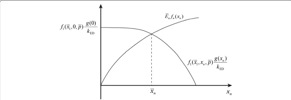
f₁ðx1;xn;pÞ⋅ gð Þxn

kED ¼

En⋅f_nð Þxn ð2Þ

which only depends on the first and the end enzyme features and is only a function of the end product con-centration xn. Usually, both f1ðx1;xn;pÞ and g(xn) are

monotonically decreasing functions of xn, which

de-scribe the negative, metabolic and gene-expression regulation, respectively. Likewise, fn(xn) is usually a

monotonically increasing function of xn. As shown by

Equation (2), the steady-state regimen corresponds to the intersection of the two functions, and is unique due to the monotonic characteristics off1,fnandg, as

illus-trated in Figure 2.

Alternatively, if theithreaction (i> 1) is product insensi-tive but the first reaction is not, thenf1is re-defined and it

also becomes a function of x2, while the kinetic function

of theithstep only depends onxi. It can be proven that at

steady state, x2 then only depends on functions f2,…,fi

and is independent of fi+ 1,…,fn−1. This conclusion is

both theoretically attractive and practically useful, because the steady state properties of an otherwise complex meta-bolic pathway may only depend on a limited number of enzyme features [33]. This is a case where the complexity of a pathway is limited; its flux and the concentrations of the upstream metabolites are only controlled by the prop-erties of the upstream enzymes and the corresponding genes.

We will now examine how metabolic control analysis and supply–demand theory deal with these types of metabolic control structures.

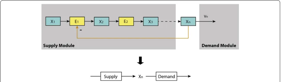
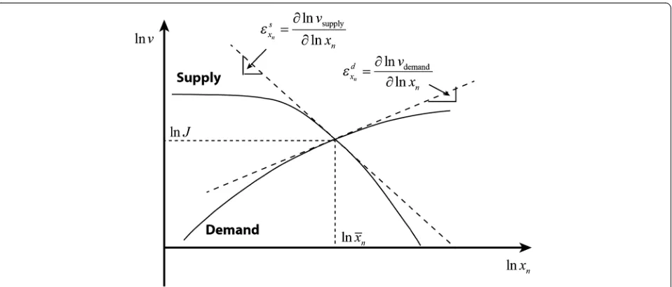
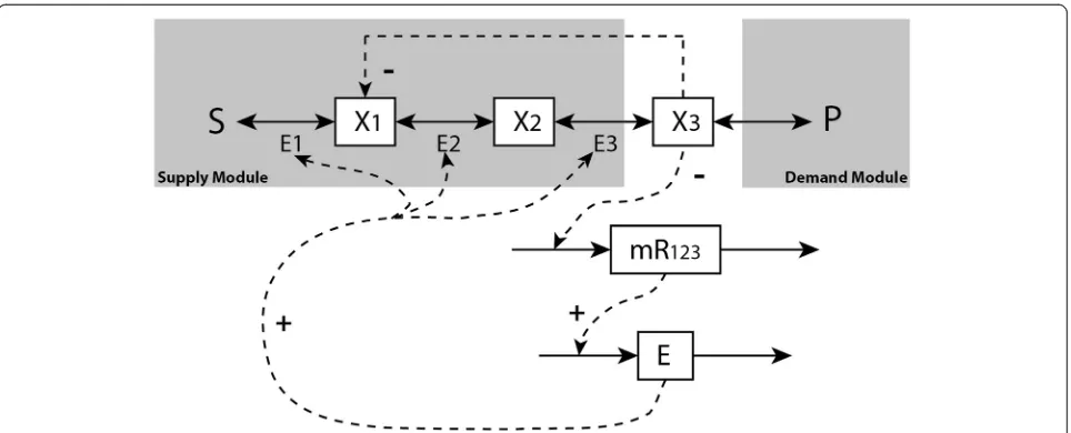
Metabolic regulation: MCA and the supply–demand theory Metabolic Control Analysis (MCA) has mostly dealt with the steady state properties of the metabolic part of Figure 1The end-product module with gene-expression and metabolic regulation.x1,x2,…,xnrepresent the concentrations of metabolites in the pathway;E1,E2,…are the concentrations of enzymes catalysing each reaction. For illustration, only the enzyme of the first reaction (E1) is

assumed negatively regulated via both metabolic (allosteric) effect and gene-expression regulation through the end productxn.

schemas such as the ones mentioned in the previous subsection. Modular MCA [34] has divided metabolic networks of this type into modules with relatively au-tonomous activities, connected through well-identified metabolites. In the supply–demand theory, Hofmeyr and colleagues [12,13] have used a similar simplification to demonstrate much of the essence of the regulation of cell function. According to the latter, the metabolic part of the end-product pathway in Figure 1 can be parti-tioned into a two-step linear pathway with supply and demandblocks as shown in Figure 3.

The concentration and flux control coefficients of metabolic control analysis measure the steady state change in the concentration of a metaboliteXand fluxJ, respectively, in response to a change in the activity of a process i. That change in activity may be effected by changing a parameterpi(e.g. concentration of an

inhibi-tor) that is specific for stepi:

CX i ¼

∂lnX ∂lnp_i

∂lnvi ∂lnp_i

¼∂_∂lnX

lnvi

CJ_i¼ ∂lnJ ∂lnp_i

_∂

lnvi ∂lnp_i

¼ ∂lnJ

∂lnvi

ð3Þ

The vi is an activity rather than the rate of reaction i

at steady state. When the parameter pi is changed, vi is

not equal to the resultant change of the steady-state rate of reaction i; it is the change in that rate only if all the other variables that affect that rate been kept constants. The concentration control coefficients of the aforemen-tioned supply–demand system can then be defined as Cxn

s ¼∂lnð Þxn =∂lnvsupply and C_dxn¼∂lnð Þxn =∂lnvdemand,

and the flux control coefficients, CJ_s and CJ_d similarly. These control coefficients describe the control exercised by a specific reaction or enzyme on the overall system variables or fluxes, while the‘local’regulatory properties of individual enzymes are quantified by the elasticity co-efficients, such as

εs xn¼

∂lnvsupply

∂lnxn ; ε

d xn ¼

∂lnvdemand

∂lnxn ð4Þ

εs xn andε

d

xn measures how the reaction rates of thesupply anddemandblocks are influenced by the end product con-centrationxn. Because the rates are those of blocks rather

than of single enzymes, these elasticities are named‘overall elasticities’ [32]. They can be further expressed into more, though not quite elemental elasticity coefficients:

εs xn¼c

J1

1 ⋅εvx1nþc J1

n−1⋅εvxnn−1

εd xn¼ε

vn xn

ð5Þ

where εv1

xn denotes the total elasticity of the first reaction with respect to xn through the metabolic regulation. The

lowercase flux control coefficientscnow refer to the local control within the supply module only (if seen as if in isola-tion withxnfixed). They can be obtained from summation

and connectivity theorems as control coefficients of the module (see Appendix B). When assuming the first reac-tion is product insensitive, thesupplymodular elasticity in (5) can be further simplified as

εs xn¼c

J1

1 ⋅εvx1n ð6Þ

In such a case, the first enzyme has the full control of flux (i.e. rate-limiting step) within the supply module, such thatcJ1

1 ¼1 and

εs xn¼ε

v1

xn ð7Þ

Using the summation and connectivity theorems in MCA, all the four concentration and flux control cients can be expressed in terms of the elasticity coeffi-cients (see Appendix B). For the concentration control of the supply step and the flux control of the demand step this becomes, using (5) and (7):

Cxn

s ¼

1 εd

xn−ε s xn

¼_εvn1 xn−ε

v1

xn

CJ_d¼CJ_vn¼ ε s xn εs

xn−ε d xn

¼ 1

1þ εd xn=ε

s xn

¼ 1

1þ εvn xn=ε

v1

xn

j j

ð8Þ These equations show that if the first reaction has complete flux control within thesupplymodule, the con-trol of steady state end-product concentration and flux are only functionally depend on two elasticity coefficients, i.e. the ones that correspond to the first and last reactions. When the feedback is very strong, i.e. εv1

xn ≫ε vn

xn , the con-trol of the demand flux CJ_d is close to 1. The MCA and supply–demand simplification thereof discussed in this section partially explain the state-steady properties of the aforementioned full regulatory system, but only for the case of metabolic regulation. When including the gene-expression regulation, a more complete interpretation can be achieved by using the hierarchical control analysis and a new‘hierarchical supply-demand’theory as investigated in the next subsection.

Gene-expression and metabolic regulation: hierarchical supply–demand theory

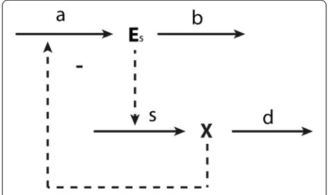
Westerhoff and coworkers have developed hierarchical control analysis (HCA), an extension of MCA that can take gene-expression regulation and signal transduction into account [14,26]. We shall here implement this by extend-ing the meanextend-ing of the elasticity coefficients in the previous subsection to include regulation through gene expressions.

When considering the metabolic part of the network alone, i.e. if gene expression were always the same, the control on the concentration of intermediateX in a sup-ply–demand system follows (8). If the roles of the synthe-sis and degradation of metabolic enzymes are considered explicitly, as illustrated in Figure 4, HCA has to be intro-duced, and the corresponding hierarchical control coeffi-cient becomes:

HX_s ¼ ∂lnX ∂lnvsupply¼

1 εd

X−

_εs

X

ð9Þ

Capital His here used for the hierarchical control co-efficients as defined in Table 1. εs

X is an“overall” elasti-city coefficient, including a classical ‘direct elasticity’ only related with metabolic responses (i.e. εs

X similar to the εs

xn defined in the MCA in (8)) and an‘indirect elas-ticity’due to gene-expression regulation:

_εs

X ¼εsXþεsEs⋅c Es a⋅εaX

ð10Þ

The lower case cis used for ‘metabolic control coeffi-cients’, i.e. control coefficients that only take the local network (metabolic, or gene expression but not their combination) into account. εs

Es is often equal to 1, i.e. when the rate of the reaction in isolation is proportional to the concentration of the enzyme catalyzing it.

Using metabolic control analysis for the gene expres-sion part of the network, the control coefficient of the protein synthesis reaction with respect to the concentra-tion of the protein synthesized is:

cEs

a ¼

1 εb

Es−ε a Es

ð11Þ

Combining the above expressions, one can express the hierarchical coefficient quantifying the control exerted by the supply enzyme on the concentration of the meta-bolic intermediate X in terms of all the elasticity coeffi-cients in the network:

HX s ¼

1 εd_X−εs

X− εs

Es⋅ε a X

εb Es−εaEs

¼ 1

εd

Xþð−εsXÞ þ εs

Es⋅ −ε a X ð Þ

εb Esþð Þ−εaEs

¼−HX d

ð12Þ The terms in parentheses are usually positive. The equation shows that the control by supply (i) decreases with the absolute magnitudes of the elasticities with re-spect toXof the supply, of the demand, and of the pro-tein synthesis, but (ii) increases for increasing elasticities of the protein synthesis and degradation reactions with respect to the concentration of the enzyme. The equa-tion also shows that for finite non-zero magnitudes of the elasticities, the hierarchical control coefficients for control by supply may be decreased by elasticities in the gene-expression network, but is usually not brought

Figure 4Illustration of hierarchical control.The lower part represents a metabolic supply_–demand system, in which the supply is catalyzed by enzymeEs(or enzymes stemming from an operon).

The upper part describes the synthesis of enzymeEsin process a

down all the way to zero. The same applies to the con-trol by demand, which is equal to minus the concon-trol by supply.

Now let us recall the end-product module with both metabolic and gene-expression regulatory feedbacks of Figure 1. As the end product (xn) regulates the first reaction

through both metabolic regulation and gene-expression regulation, the corresponding‘overall’elasticity (see Table 1) of the first reaction can be expressed as:

_εv1

xn ¼ε v1

xnþε v1

E1⋅c

E1

vTrans⋅ε

vTrans

xn

ð13Þ

where εv1

xn denotes the elasticity through metabolic regula-tion,cE1

vTransdenotes the control of gene expression (i.e.

tran-scription and translation) on the concentration of the first enzyme [15,35]. By replacing the εv1

xn in (7) with the more complete expression (13), i.e. using εs

xn ¼ _εv1

xn, the hier-archical control coefficientHxn

s can be expressed into elas-ticity coefficients, in a similar manner as (12). Since both metabolic and gene-expression regulation constitute nega-tive feedbacks,εs_xn is negative and becomes more negative with increasing xn due to increasing product inhibition.

εd

xn is positive and decreases asymptotically to zero with increasing xn. Therefore, the relationship between

the reaction rate and end product concentration can be described in terms of the elasticities as depicted in Figure 5. Figure 5 explains the unique steady-state results obtained from classical steady state analysis (see Figure 2).

An illustration of the supply–demand relationship similar to Figure 5 has been presented in [13]. However, here we extend the interpretation of the system and cor-responding elasticity coefficients to the more general case that includes gene-expression regulation. As an ex-tension to the classical supply–demand theory, the ana-lysis given in this section can be named the‘hierarchical supply-demand’theory.

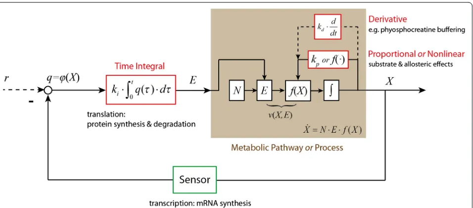
Control engineering

The discipline of Control Engineering first identifies a so-calledcontrolled variable, which it sees as the output of the system. In metabolic biochemistry, output often relates to a flux, but can also be the concentration of an important metabolite in the pathway. Control engineer-ing next examines the various categories of mechanism that may contribute to the capability of the network of Table 1 The list of symbols and definitions

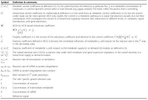
Symbol Definition & comments

Cf_i orcf

i Metabolic control coefficients as defined in (3).fis the system function of interest (i.e. a particular flux,Jj, or a metabolite concentrationX). Lowercasecis used to represent control within a local network (e.g. supply module). The indexirefers the process that is controlling.

Hf

i Hierarchical control coefficient. Its mathematical definition is in the same form as metabolic control coefficients in (3), but the system under study can be more general. MCA only studies the control in a metabolic pathway or a signal transduction cascade, but not their combination. HCA investigates the control in a hierarchical regulatory network with interactions at different levels, i.e. metabolic, signal transduction, and gene-expression.

ℜf

i MCA (or HCA) based robustness coefficient.

ℜf

i≡ 1

∂lnf

∂lnei

≡1

Cf i

or 1

Hf i

.

Ff

i Fragility coefficient. It is the inverse of the robustness coefficient and identical to the control coefficient.Ffi≡∂∂lnlnefi≡

1

ℜf i≡

Cf i or Hfi: εvj

xi Elasticity coefficient defined in MCA. It denotes the immediate influences of metabolitexiwith respect to the reaction rate in thej

th_step

in the pre-steady state. εs

xi orε

d

xi Elasticity coefficient of metabolitexiwith respect to the metabolic supply (s) or demand (d) module, as defined in (4).

_εvj

xi,ε

s xi

(orεd xi)

The overall elasticity (see [32]) for a reaction step under both metabolic and gene expression regulation, or the overall elasticity in a hierarchical supply or demand module.

vTrscor

vTrnl

Reaction rate of transcription or translation

vRDorvED Reaction rate of mRNA or protein degradation

kRDorkED mRNA or protein degradation rate constant

ki_proteolysis Rate constant ofithorder proteolysis μ The cells’specific growth (division) rate E Concentration of enzyme

X or xi Concentration of intermediate metabolite

R Concentration of mRNA

maintaining the controlled variable close to its original steady state value when the system is subject to a sus-tained perturbation. The ‘error (function)’ is the devi-ation (δX) of the value of the controlled variable (X) from its value before the perturbation, or the difference to a reference signal r. The network ‘adapts’to the per-turbation of the controlled variable, i.e. to the error function, in a so-called‘control action’. RNA polymerase plus the ribosomes that together translate changes in the concentration of metabolites to changes in gene expres-sion, or direct metabolic regulation of the activity of an enzyme correspond to such control actions. The output of the control action (or of the ‘controller’) is often named the manipulated variable. In metabolism, reac-tion ratesv(X,E) are variables manipulated either by the concentration of metabolites (f(X)) or by the tion of the enzyme that catalyses the reaction concentra-tion (E). A mechanical control system often includes an actuatorthat converts the control signal into some kind of mechanical motion. For a biochemical system dis-cussed in this study, this may correspond to the enzyme catalysing the reaction synthesizing or degradingX. Usu-ally there exists asensormeasures the controlled variable and translates its error function into the input signal of the controller. In a gene-expression regulation, the tran-scription factor can be regarded as the sensor.

The three most widely used categories of control are the proportional, integral, and derivative (PID) control mechanisms [17]. They differ depending on whether the control system’s response is a function of the ‘error function’ itself, the time integral thereof or the time derivative thereof, respectively. In systems biology literature, the proportional control mechanism

has already been referred to in terms of metabolic regulation [19,20,23] (e.g. feedback inhibition). However, when Control Engineering discusses proportional control mechanisms, response is proportional to the error func-tion. In actual biochemistry, enzyme activity is rarely a linear function of the concentrations of metabolites X, which includes the enzyme’s substrate, its product and allosteric modifiers. MCA accommodates this nonlinearity by allowing the elasticity coefficient to differ from 1. Metabolic regulation by the‘error function’, is part of the nonlinear dynamics of the process or system, i.e. f(X), both conceptually and in the mathematical modelling. It would seem therefore that the proportional control of Control Engineering can be nonlinear in biochemical networks.

Integral control action through the accumulation of molecules in the metabolic process has also been reported [19,20,23]. Here the systems response should be a function not of the error function itself but of the integral of that error function. In the present study we examine gene-expression regulation from this point of view, since pro-tein synthesis requires time integration and depend on the error function, and because changes in protein concentra-tion directly affect the rate of the reacconcentra-tion the protein may catalyzes. We may expect that this integral control some-how corresponds to the ‘indirect elasticities’ of HCA. Whether indeed gene-expression regulation corresponds to an exact (or ideal) integral control mechanism will be further discussed in the Results and Discussion section. Whether there exists a derivative control action and whether it relates to a specific type of regulation in a meta-bolic pathway will not be investigated in this paper. Refer-ence [23] already identified an example.

Considering the dynamics of a metabolic system, we can write the time dependence of the concentrations of its metabolites as:

_

X ¼N⋅v Xð ;EÞ ¼N⋅E⋅f Xð Þ ð14Þ

N is the stoichiometry matrix. E is a diagonal matrix with the concentrations of the enzymes that catalyse the various reactions along its diagonal. f(X) is a vector function of the concentrations of the metabolites and kinetic parameter values. The regulated metabolic path-way can be described in terms of a closed-loop feedback control system, as indicated in Figure 6, in whichkp, ki

and kd are the PID control parameters. We here note

that Figure 6 and subsequent figures refrain from bio-chemical detail. This is because the analysis in the present paper aims at obtaining a set of conclusions with general significance. Being specific in the schemes we use as illustrations would detract from this aim.

When considering a sustained perturbation γ∙δp (e.g. change in a parameter p) and denoting by δthe (small) deviation from the steady state prior to this perturb-ation, the time dependent variation in the metabolite concentrations may be observed:

δX_ ¼N⋅δv Xð ;EÞ ¼N⋅Ess⋅f′ð ÞX⋅δXþN⋅f Xð Þss⋅δEþγ⋅δp

ð15Þ

The subscript ss refers to the steady state values. By substituting the time integration of gene expression, i.e.

ki⋅Z t 0

qð Þτ ⋅dτ, for δE, and assuming the proportional

and derivative actions a part of the metabolic process (14),

δX_¼N⋅Ess⋅f′ð ÞX ⋅δXþN⋅f Xð Þss⋅ki⋅ Z

0

δφð ÞX ⋅dtþγ⋅δp

ð16Þ

This describes the overall dynamics of a closed-loop metabolic system under perturbation as a sum of three terms. The first term of these is a nonlinear function of (or in first order proportional to) the perturbation of the controlled variable (i.e. the error function)δX. This term describes all the direct elasticities, including non-regulatory system kinetics such as substrate and product effects, and (other) metabolic regulation such as allosteric activation. The second term corresponds to a time integral of a func-tion of the perturbafunc-tion of the controlled variable δX, and can also depend on other system variables as discussed in the Results and Discussion section.

We shall now examine whether these two terms in the equation (16), correspond to the proportional and integral control loops of Control Engineering.

Results and discussion

A simple example of combined metabolic and

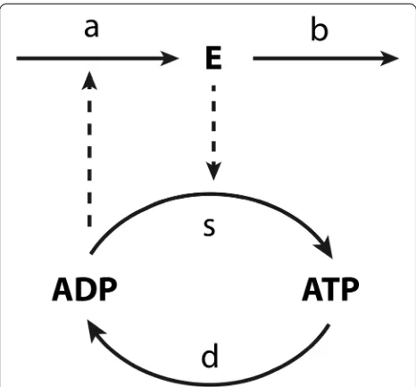
gene-expression regulation of an important intracellular process: ATP (energy) metabolism

Let us consider the simple example given in Figure 7, i.e. a two-step pathway with ATP and ADP as combined intermediate and with the expression of the gene encod-ing the first enzyme E increasing in proportion to the concentration of ADP. The‘moiety conservation sum’C is the sum of the concentrations of ATP and ADP and a constant here (i.e. C= [ATP] + [ADP]) because the reac-tions only convert the one into the other. The metabolic regulation addresses the interplay between the supply and demand processes (sandd).

The dynamics of ADP and enzymeEare here assumed to follow mass action kinetics:

d ADP½ =dt¼−ks⋅E⋅½ADP þkd⋅ðC−½ADPÞ

dE=dt¼ka⋅½ADP−kb⋅E−k0

ð17Þ

The degradation of the enzyme is here written as the sum of two terms, which will serve to emphasize the im-plication of this degradation to be independent (forkb= 0)

or dependent (for k0= 0; see below) on the enzyme

con-centration. The first order degradation rate reflects the

assumption that there is a rather unspecific protease activ-ity for which the particular enzymeE we are considering here is a minority substrate. The zero order degradation would reflect a case where there is a specific protease system for enzymeE(e.g. an ubiquitination followed by a generic protease) that is saturated by the already high concentration of the enzyme relative to theKMof the

ubi-quitin transferase. In (17) all rate constants are considered non-negative and k0= 0 wheneverE is non-positive. The

closed-loop control system structure of the pathway can be represented as in Figure 8.

The control system diagram suggests that the ADP concentration is the controlled variable and the en-zyme concentration E a manipulated variable in the gene-expression control loop. The zero order degrad-ation rate k0 can be treated as a reference signal to

the system. The metabolic regulation is included as a part of the ADP kinetic process. By considering a perturbation of kd from its steady state value (i.e.

δkd), and reformulating the kinetics of ADP and E

(see Appendix C), we have

δ½ADP: ¼−ðks⋅EssþkdÞ⋅δ½ADP−ks⋅½ADPss⋅ Z ∞

0 ka⋅δ½ADP−kb⋅δE

ð Þ⋅dt

þC−½ADP_ss ⋅δkd

ð18Þ Comparing this to a general closed-loop control system (16), with ADP forX, we recognize on the right-hand side first a proportional response term, then an integral response term, and then the perturbation term. The proportional response corresponds to the direct

‘elasticity’ of the supply and demand reactions with re-spect to the error functionδ[ADP], which is a metabolic and instantaneous regulation. The integral response is related to the protein synthesis and degradation and thus to gene-expression regulation.

When the degradation of enzyme is zero order in terms ofE(i.e. whenkb= 0), the gene-expression regulation

be-comes an ideal integral control loop, and the metabolic network can exhibit robust perfect adaptation to the exter-nal or parametric perturbations. This can be understood by requiring (18) to be valid in a steady state, i.e. with time independent values for [ADP] andE.Because the time in-tegral reaches to infinity this requires that the argument of the integral, i.e.ka⋅δ[ADP]−kb⋅δE, must equal zero. The

mechanism for this perfect adaptation is that after the per-turbation the concentration of the enzyme will vary until it makes the time dependences equal zero by itself, forgo-ing the more usual process in metabolic regulation that changes in the controlled variable arrange for the steady state to be re-attained in the presence of the sustained perturbation.

For the more general case where the enzyme degradation may depend on the enzyme’s concentration, the (hierarch-ical) control of the enzyme level by the demand reaction can be expressed in terms of the kinetic parameters and the steady-state ADP concentration (see Appendix C):

HE_kd ¼ ∂lnE ∂lnkd¼

ks⋅ka

kb ⋅ ½ADPss

2

kd⋅Cþks⋅½ADP_ss 2⋅ka kb

¼1− 1

1þks⋅ð½ADPssÞ 2

kd⋅C ⋅ ka kb

ð19Þ

The flux control exercised by the demand reaction is quantified by:

HJ_kd ¼ ∂lnJ ∂lnkd¼1−

ADP

½ ss C

1þks⋅ð½ADPssÞ 2

kd⋅C ⋅ ka kb

ð20Þ

Both the control of enzyme level and the control of de-mand flux by the perturbation equal 1 minus a hyperbolic function of kb. For the ideal integral control scenario of kb= 0, the enzyme concentration E tracks the activity of

the pathway degrading ATP perfectly, i.e. HE

kd¼1. More importantly, the pathway flux perfectly tracks the perturb-ation in the demand flux andHJ_k

d ¼1. This is the case of robust perfect adaptation. For other cases whenkb≠0, the

adaptation of the pathway to the perturbation will not be perfect and both control coefficients are smaller than 1.

Also the robustness coefficient [36] of the ADP con-centrations vis-à-vis perturbations in the demand reac-tion can be expressed in terms of kinetic constants and the concentration of ADP (see Table 1 for definition):

ℜ½ADP

kd ¼

1

∂ln½ADP

∂lnkd

¼kd⋅Cþks⋅ ½ADPss

2

⋅ka kb C−½ADP_ss

⋅kd

ð21Þ

Only ifkb= 0,kd= 0, or [ATP]ss=0, the ADP and ATP

are perfectly robust (ℜ½_kADP_d ¼∞) versus perturbations.

The fragility [36] of the ADP concentrationvis-à-vis per-turbation in the demand reaction, which is the inverse of the robustness, can be quantified by the concentration control coefficient for the concentration of ADP with re-spect to the degradation process. It reads as:

F½_kADP d ≡1=ℜ

ADP

½

kd ¼

∂ln½ADP ∂lnkd ¼

C−½ADP_ss

Cþ½ADP_ss 2⋅ks⋅ka kd⋅kb ð22Þ

This fragility is a hyperbolic function of the first order degradation rate constant of the enzyme and hence zero when that degradation is zero-order (see Figure 9 for il-lustration). The fragility has the ATP/(ADP + ATP) ratio as its maximum value (hence the minimum robustness equals the (ADP + ATP)/ATP ratio). Half maximum fra-gility is attained for:

kb¼ ½ADPss

2

C ⋅

ks⋅ka

kd ð23Þ

This means that the fragility may be low for a substan-tial magnitude of the first order rate constant of protein degradation if the rate constant for protein synthesis is also high. The control coefficients for the enzyme level HE

kd and the demand flux H J

kd attain a maximum of 1 and a value of ½ when the fragility of ADP is half maximal.

These conclusions can be generalized somewhat by directly implementing HCA and hierarchical supply– de-mand result given in (12). For the above model the elas-ticity coefficients assume the following magnitudes:

εs ADP

½ ¼εa½ADP¼ε s E ¼1

εa E¼0

εd ADP

½ ¼−

ADP

½

C−½ADP

ð24Þ Figure 8Control system structure of ATP energy metabolism.k0andkbare the zero and first order protein degradation rate constants.kais

For the robustness of the ADP concentration vis-à-vis increased demand one then finds:

1 H½_dADP¼−ε

d ADP

½ þεs½ADPþ εs

E⋅εa½ADP εb

E−εaE

¼_C−C

ADP

½ þ

1 εb E

ð25Þ

This shows that robustness is infinite if the enzyme degradation reaction is zero order (i.e. εb

E¼0), and that the robustness becomes smaller with increasing order (elasticity) of this reaction.

The most important conclusion here is that there is no discontinuity in the ability of integral control loops to lead to good adaptation. The closer the degradation of the enzyme that enables the adaptation is to a zero-order reaction, the stronger its tracking of the perturb-ation in the demand flux, and the higher the robustness of the variable that is to be kept homeostatic. Important perhaps is the phenomenon that the robustness is not determined by the magnitude of the degradation reac-tion but by its kinetic order (i.e. elasticity of effective Hill coefficient). The corresponding conclusions pertain to the tracking of the demand by the enzyme level E and the control of the pathway flux by the demand reaction.

A further issue in control engineering is the robustness of systems versus perturbations at various frequencies. In engineering, an airplane wing has to be robust to vari-ations of air pressures at high frequencies, as well at low frequencies. In order to achieve this combined robust-ness, different control loops may have to be put in place simultaneously, although a trade-off limits what one can

do [18]. In systems biology, this can be illustrated for the end-product feedback regulation in Figure 1. If the flux demand of the pathway increases rapidly, the concentra-tion of the end product decreases rapidly and as a result of the direct allosteric product inhibition effect, the ac-tivity of the first enzyme will increase quickly too. This metabolic control of enzyme activity is a fast actuator of the system. However, if there is a further increase in the flux demand, the first enzyme may‘lose’its control cap-acity since its activity may be approaching its maximum capacity (kcat). At this stage, the system may then

undergo a second ‘adaptation’ through gene expression which should be expected to be slower because the cell has to produce enzyme, but still ultimately lead to an increase in the concentration of the first enzyme. This increase should then decrease the direct metabolic stimulation of the catalytic activity of the enzyme dis-cussed above. In this sense, the regulation of the first en-zyme of the pathway is bi-functional in dynamic terms [18]: The metabolic regulation rapidly rejects high fre-quency perturbations but possibly with small amplitude or capability, while the gene-expression regulation is slow to adapt, but may be able to reject very large con-stant perturbations.

Conditions for integral and pseudo-integral control: end-product pathway

In this section, we recall the end-product module ex-ample (of which the simple ATP metabolism exex-ample is a special case) to analyse gene-expression regulation in a more general metabolic pathway. In particular, the con-ditions will be identified for which the gene-expression regulation constitutes ideal integral control or pseudo-integral control will be discussed. A simple but represen-tative end-product example is given in Figure 10, i.e. a linear pathway with three metabolites, where for all the three enzymes the gene expression is regulated by the last metabolite. The kinetic model of this example with all the parameters is provided in [5].

Gene transcription and translation are modelled here explicitly by further including the dynamic function of mRNA as

_

R¼vTrsc−vRD¼gTrscð Þx3 −kRD⋅R

_

E ¼vTrnl−vED¼gTrnlð ÞR −kED⋅E ð

26Þ

HeregTrnl(R) =kTrnl⋅Ris a function of mRNA

concen-tration R. kED essentially consists of three parts. One

term is due to dilution, which is proportional to the spe-cific cell growth rate μ. The other terms correspond to proteolysis, as below:

kED¼μþk1proteolysisþk 0

proteolysis=E ð27Þ

The final term denotes the zero order proteolysis as would be caused by proteases that are saturated with the protein of interest. We here assume that the specific growth rateμis independent of the activity of the path-way under study, an assumption that is sometimes but not always realistic. Since after multiplying with E the last term is independent of the protein concentration, it is convenient to move this term into the protein syn-thesis function gTrnl(R). Hence, the new protein

degrad-ation rate can be defined as,

kED¼μþk1proteolysis ð28Þ

and the protein dynamics can be re-written as,

_

E ¼g_Trnlð ÞR −kED⋅E

¼ kTrnl⋅R−k0proteolysis

−μþk1_proteolysis⋅E ð29Þ

In the exponential growth phase or if proteolysis is first order (i.e. kED≠0), the above pathway example

corresponds to a pseudo- or non-integral control scenario. The control structure of the regulatory system is then given by Figure 11. The dynamics of the ‘sensor’ is decomposed here by addressing both transcription and the translation through mRNA. At steady state, often gTrnl(R)ss=kED⋅Ess≠0. Therefore, after

perturb-ation of a system parameter (i.e. kinetic constants), the new steady state values of x3, R, and gTrnl(R) will

no longer be the same as the old steady state values, which indicates that then the regulatory system does not achieve perfect adaptation. However, when kTnD is

very small, near-perfect adaptation behaviour should be observed.

An ideal integral control scenario will happen only when cell enters a stationary phase and there only exists zero order proteolysis, i.e. kED¼μþk1proteolysis¼0 . In

such case, at steady state, gTrnl(R)ss≡0 due to integral

control, and R and x3 will also always keep the same

constant values at steady state, no matter how the sys-tem parameters are perturbed. The adaptation of the system is then perfect in the sense of making the system properties R and x3 robust against the perturbations.

The functions gTrnl(·) and gTrsc(·) can also be

multivari-ate, i.e. contain other system variables. Only if those var-iables do not depend functionally on the protein concentration (E), the adaptationvis-à-vis perturbations of the system kinetic parameters will remain perfect.

The ideal integral control scenario that we considered above led to the perfect robustness of certain system variables with respect to certain (external or parametric) perturbations. A second aspect of the perfect adaptation scenario is the perfect tracking by a second system vari-able of perturbations. Perfect tracking means that the relative change in the variable is identical to the relative change in the perturbing parameter. If the parameter is the activity of a process, then this means that the corre-sponding control coefficient is equal to 1. The perfect tracking of references and the perfect robustness of con-trolled variables to perturbations are two aspects of inte-gral control systems, i.e. the two features can be observed simultaneously for the same system. A specific pathway then shows perfect robustness of a system vari-ablevis-à-vis multiple perturbations (or parameters) but perfect tracking with respect to only a limited set of pa-rameters (e.g. a reference signalr).

Figure 10A linear end-product pathway with gene-expression and metabolic regulation.The metabolites are denoted byxi, mRNA by mR and enzymes by E. S and P are the external metabolites. Metabolitex3inhibits the rate of enzyme 1 through metabolic regulation and the

For the aforementioned example, the zero order proteoly-sis can be regarded as a‘reference’signalr¼k0_proteolysis. Ef-fectively perturbation of this rate constant corresponds to an external perturbation of protein synthesis. The effect is that even at an ideal integral control case, i.e. whenkED= 0,

the steady state concentration of mRNA will not become 0. Rather, it will always‘track’the referencer(i.e.R=r/kTrnl≠

0) wheneverE_ss¼0. The reference tracking control system structure is included in Figure 11 with referencerreferred to by a dashed arrow, and withgTrnl(R) then representing

kTrnl⋅R.

Practical concerns and assumptions on degradation rate constant kED

In general, kED¼μþk1proteolysis>0 . It may seem that

the condition of integral control can be approached, when either i) kED< < α with α a very small positive

value, or ii) kED< < kTrnl (or kED· E< < gTrnl(R)). In the

latter case, for the level of protein to remain bounded, there should be a background degradation rate of the protein independent of the concentration of that protein. This would be so if:

μþk1_proteolysis≪k0_proteolysis=E ð30Þ

During the exponential growth phase of bacteria such asE. coliless than 1% of a protein may be degraded dur-ing a cell division cycle [37]. Consequently the major term in the protein degradation is the dilution term μ and this term is generally very small. Indeed, by defin-ition, eμ⋅T= 2, whereT is the doubling time of the bac-teria and then μ= ln2/T. Practically, the smallest value

for T is close to 20 minutes [38], which corresponding to the fastest growth rate ofE. coli:

μ≈ln 2=ð2060Þ ¼5:810−4 s−1 ð31Þ

Such a growth rate in microbes such as E. coli and yeast, which is fast for organisms but slow at the time scale of RNA and protein synthesis, produces a small ef-fective degradation rate constant for the proteins. Below we shall see whether such a small degradation rate constant suffices to produce near-perfect adaptation behaviour in practice, which would be interpreted as a quasi-perfect integral control system.

Simulation study

In this section, both the integral and the non-integral con-trol scenarios are simulated based on the example given in Figure 10 with all the kinetic parameters given in [5]. Three different systems are considered, withkED= 0, 0.2, and 0.4,

respectively. All three systems are simulated from the same initial condition. The concentration changes of mRNA, E andx3are shown in Figure 12. After a period of time (e.g.

30 seconds) the three systems reach different steady states. Then at 50 seconds we perturb one system parameter (i.e. the kcat of the third reaction) by 20% for all three cases.

After a while the three systems reach new steady states. After perturbation only the system with zero order protein degradation (i.e.kED= 0), returns to the same steady state

values for mRNA and x3 as those before perturbation,

which indicates perfect adaptation: this is an ideal integral control system. In this case the manipulated variable, the enzyme levelE, varies strongly. Its adaptation enables x3 and mRNA to be completely robust vis-à-vis the

Figure 11Control system structure of a pseudo-integral or an ideal integral control problem.hTrsc(·) denotes the transcription process.

gTrnl(·) denotes the rate of protein synthesis. The pseudo-integral control system becomes an ideal integral control only when the dashed line

perturbations of thekcatof the third reaction. In the other

two cases (i.e.kED= 0.2 or 0.4), the change in enzyme level

is smaller, but the new steady state values of mRNA and x3 deviate from their previous steady-state values and

adaptation is not perfect. However, the deviations are not large; only 3% for x3and 4% for mRNA when kED= 0.2,

and 4% forx3and 8% for mRNA whenkED= 0.4.

Now let us consider the reference tracking scenario. The responses of enzyme and mRNA to a 20% perturb-ation in the protein stability (r) at t= 50 seconds, are given in Figure 13 for three different rate constants of enzyme degradationkED. Only when kED= 0 the mRNA

concentration tracked the reference value with zero steady state ‘deviation’. This indicates the existence of a perfect integral action of the feedback regulatory system. When kEDwas not equal to zero (i.e. kED= 0.2 orkED=

0.4), the mRNA response did not track the reference sig-nal, indicating that in these two cases the controller of the system was not an ideal integral controller, although it changed less than did the reference signal.

HCA and an hierarchical supply–demand interpretation This simulation example can be represented by a hier-archical supply–demand structure such as in Figure 4. To obtain ideal integral control, both protein synthesis and protein degradation should be independent of the concentration of the protein that is being degraded (i.e.

_

E ¼g_Trnlð ÞR). Since this implies that protein degradation is zero order in protein concentration:

εb Es¼ε

a

Es¼0 ð32Þ

So that the hierarchical control coefficient of the me-tabolite concentration becomes

HX_s ¼ 1

εd X−εsX−

εs Es⋅εax

εb Es−εaEs

¼ 1

εd

Xþð−εsXÞ þ εs

Es⋅ −ð Þεax

0

¼0

ð33Þ

Here εa Es¼ε

vTrnl

E , εbEs ¼ε vED

E , HXs ¼H x3

3 for the

biosyn-thetic pathway example. Because the hierarchical control by supply and demand must add to zero (due to the concentration control summation law [15]), also the control by demand on the metabolite concentration be-comes precisely equal to zero in the zero order protein degradation case.

Feed-forward activation: a case study of a leucine biosynthetic pathway

In previous sections, either a metabolic intermediate (ADP) or a penultimate product (xn) inhibited or

re-pressed upstream enzymes. In this section a different regulatory structure is investigated, one in which a metabolite activates downstream enzymes through gene-expression. A simplified mathematical model de-scribing the leucine biosynthetic pathway in Saccharo-myces cerevisiae [39] is used to demonstrate that the analysis integrating hierarchical supply–demand the-ory and control engineering continues to apply. The pathway converts pyruvate to leucine by the sequen-tial reactions described in Figure 14. There are two major regulatory mechanisms in the pathway. One is a metabolic feedback inhibition of Leu4 and Leu9 by leucine, which is an end-product module similar to the ones discussed above. The other is the transcrip-tional (gene-expression) activation of downstream en-zymes Leu1 (E1) and Leu2 (E2) by αIPM (I1) (through

transcription factor Leu3), which we shall call initial-product modules (see Appendix A and Figure 17). The model predictions fit the experimental data and all the parameter values have been estimated and provided in [39].

The hierarchical control coefficient quantifying the con-trol of supply enzymesEswith respect to the concentration

ofI1(αIPM) can be expressed into the various elasticity

HI1

s ¼

1 εd

I1þε

d E1c

E1

a1ε

a1

I1 þε

d E2c

E2

a2ε

a2

I1

−εs I1

¼ 1

εd I1−ε

s I1þ

εd E1⋅ε

a1 I1

εb1 E1−ε

a1 E1

þεdE2⋅ε a2 I1

εb2 E2−ε

a2 E2

and its value can be computed from the simulation of the pathway model by perturbingEuand recording the changes

in the steady state value ofI1. This led toHIs1¼0:12. The hierarchical control coefficient is small but not zero, which indicates that the regulatory network can react and adapt to this external perturbation although the adaptation is not

‘perfect’.

The closed-loop control system structure of the down-stream gene-expression activation is the same as that of the upstream inhibition case described in Figure 11 (with end-product metabolic regulation dominating process dy-namics). It is still a negative feedback control rather than a

feed-forward control in the control context: For anegative feedback control system, a change (increase/decrease) in some controlled variable will result an opposite change (decrease/increase) in the operation of the process itself in such a way as to reduce changes. For the end-product module given in (1), when E1 increases the

concentra-tion of the end product xn also increases, whilst as xn

increasesE1would decreases as a result of negative feedback

inhibition (through metabolic or gene-expression regula-tion). Hence this is a negative feedback control system, since when E1increases the system attempts to reduce such an

increase. For case of the positive activation of down-stream enzyme by a metabolite updown-stream of that enzyme (i.e. initial-product module given in (34)), whenE1increases

the concentration of x1 decreases since it is a

down-stream enzyme, while E1 would also decreases as x1

decreasing because of the positive feed-forward activation. This gives the same result as the end-product case.

Figure 14A schematic diagram of the simplified leucine biosynthetic pathway model.Eurepresents Leu4 and Leu9,E1represents Leu1,E2

represents Leu2,I1andI2denoteαIPM (α-isopropylmalate) andβIPM respectively. The source is pyruvate andPrepresents leucine. The supply

and demand modules of the pathway are shown in shading.

Figure 13The responses of enzyme (E) and mRNA concentrations with differentkEDvalues.First the reference signalrwas set to 0.5. By adjusting the protein synthesis rate (ktrnl), the same steady state values of mRNA (i.e. mRNAss= (kED·Ess+r)/ktrnl= 0.5) and enzyme concentrations

Herewith, both two systems are negative feedback control system in the control context and both can be represented by the same feedback control structure as given in Figure 11.

In this model, the protein degradation rates purely de-pend on the dilution effects, and the estimated growth rate of μ= 0.0058 min-1= 9.7 × 10-5s-1 is very small as compared to metabolic turnover times and may imply the existence of a quasi-integral control scenario. For testing, a simulation study is provided where a 50% in-crease on the kcat of the first reaction is applied at

800 minutes as an environmental perturbation, the cal-culated concentration changes of the intermediate me-tabolites are shown in Figure 16. This perturbation could be due to an allosteric activation by a substance added to the system. The concentrations of both αIPM

and βIPM reach new steady states. The differences

be-tween the new and the old steady-state values are around 7% and 20% respectively. Again, the adaptation is imperfect; the two concentrations are robust but not infinitely so.

Conclusions

In this paper, two existing approaches to the analysis of the robustness and adaptation of networks have been inte-grated: control engineering and MCA. The former designs control structures for networks that lead to optimal behav-iour, for instance in terms of ‘perfect adaptation’leading to infinite robustness. The latter quantifies the extents to which processes in a network determine fluxes and concen-trations and identifies the molecular interactions that deter-mine the corresponding distributions of control. Two extensions of MCA have also been integrated into our ana-lysis, i.e. HCA adding the possibility to analyse regulation through gene expression, and supply–demand theory,

greatly simplifying the analysis towards understanding of the essence. We also integrated the two latter approaches into a novel hierarchical supply–demand theory. The steady state properties of exemplary metabolic pathways served as test cases; they were analysed in terms of the robustness of their steady state properties. They included a pathway of free energy transduction, a pathway with feedback inhib-ition and repression, and a pathway with feed-forward regu-lation. Most substrates for the synthesis of macromolecules such as proteins and nucleic acids are the end product of such pathways, making this analysis important for the un-derstanding for the control of cell growth.

We then used the resulting framework to address the question whether metabolic pathways regulated by both metabolic interactions and through gene expression, come close to the ideal control structures designed in control engineering. We focused on the control structures leading to so-called‘perfect adaptation’, as defined by (i) complete robustness of the concentration of the pathway’s end product towards perturbations in supply and demand, (ii) perfect tracking of perturbations by variables involved in the adaptation. Control engineering distinguishes between proportional, derivative and integral control and showed that of these only integral control loops produce perfect adaptation. In a hierarchical control analysis, in a hierarch-ical supply–demand analysis, as well as in a number of computer simulations, we showed that such perfect adap-tation (and perfect tracking) should not be expected for the usual gene-expression regulation pathways, even though they seem to engage in integral control. Although that integral control increased the robustness of the con-centration of the pathway product vis-à-vis perturbation in the activities of metabolic enzymes, that robustness was not perfect, except for the singular case where the meta-bolic enzymes would be infinitely stable. For complete steady states, such infinite stability should not be consid-ered realistic.

We expected that for cases where proteins are highly, adaptation of the anabolic networks studied should be high even if not quite perfect. This was however not much ob-served. HCA can show that this is not to be expected ei-ther. The perfectness of the adaptation of the networks in complete steady state should not be a function of the mag-nitude of any first-order protein degradation rate constant, but rather a function of the order of the protein degrad-ation reaction, or to be precise, of its elasticity coefficient: the protein degradation should be zero order in protein concentration for the adaptation to become perfect.

Because gene expression regulation involves a time inte-gral that is a function of changes at the level of the meta-bolic pathway, we suggest that at least when applied to biological systems, control engineering is extended so as to explicitly include such ‘integral control’ loops even if they do not lead to perfect adaptation. By adding the Figure 15Illustration of the hierarchical supply–demand

structure of the leucine biosynthetic pathway.a1and b1denote

the synthesis and degradation of enzyme Leu1 (E1); a2and b2

denote the synthesis and degradation of enzyme Leu2 (E2). s and d

subtlety of HCA one can then analyse how perfect the adaptation furnished by the integral control loop actually is. We propose a simplification of the control-engineering concept of ‘proportional control’to the more general case where the adaptation is any function of the displacement of the controlled variable but neither a function of the time integral nor the time derivative of that displacement. That function could be more complex than the propor-tionality used in control engineering and thereby be realis-tic for biochemical networks, thereby making control engineering much more useful for the life sciences. Per-haps the terms ‘proportional control’should then be re-placed by ‘direct or metabolic control’, referring to the direct nature of the interactions.

Metabolic networks typically have more than one meta-bolic intermediate and when the network is perturbed by affecting a process activity, many metabolite concentra-tions tend to change. If it is of particular interest to main-tain one of these as constant as possible whereas variations in other metabolite concentrations are less det-rimental to biological function, then the former may be designated as the‘controlled variable’and the latter as‘ ma-nipulated variables’in the control engineering analysis. Be-cause many enzymes do not serve a function other than through the reaction they catalyse, they may be the more obvious‘manipulated variables’. On the other hand it may well be that some metabolite concentrations serve as‘ ma-nipulated variables’ with the sole function of providing near perfect control loops. cAMP might be an example.

Integral control loops do not require gene-expression regulation. Also in exclusively metabolic networks, integral control may arise. An example would be a linear pathway with the penultimate metabolite affecting the first reaction of the pathway, whilst its degradation rate is independent of its concentration. If the first step of the pathway is then perturbed, the concentration of the penultimate metabol-ite will be a function of the time integral of the

perturbation of the first metabolite concentration in the pathway, and it may effect perfect adaptation. On the other hand, if the degradation rate of that penultimate me-tabolite were first order, then that concentration would be a direct function of the concentration of the first metabol-ite of the pathway, and the regulation would turn into pro-portional rather than integral control. In hindsight, reference [33] was an early example of this.

As shown at length in the present paper, gene-expression regulation does not always lead to perfect adaptation. Indeed, if protein degradation is first order, then the deviation in the concentration of the enzyme may well be proportional to the perturbation in the con-trolled variable and one effectively obtains ‘proportional control’ through gene-expression regulation. We con-clude that whether control loops correspond to the inte-gral or proportional category of control engineering depends on the elasticity coefficients (orders) of the re-actions involved with respect to the controlled variable, rather than on time integration being involved. The ex-tension of control engineering with hierarchical control analysis that was initiated here, may well provide the subtlety that helps analyse the complex networks that mankind is confronted with today, both in the life sci-ences and in economics and environmental scisci-ences. It may also help design new and better networks, if only for synthetic biology and biotechnology.

network structure that control engineering may come up with as serving a function of coordination. And it will be of interest whether this type of network may serve a similar function in Biology.

Appendices

A. The initial-product module

The initial-product feed-forward regulation module given in Figure 17 can be mathematically described by the following differential equations:

_

x1ð Þ ¼t v0ð Þt −E1ð Þt f1ðx1ð Þt ;p tð ÞÞ

_

x2ð Þ ¼t E1ð Þt f1ðx1ð Þt ;p tð ÞÞ−E2ð Þt f2ðx2ð Þt ;x3ð Þt Þ

⋮ ⋮ ⋮

_

xnð Þ ¼t En−1ð Þt fn−1ðxn−1ð Þt ;xnð Þt Þ−Enð Þt fnðxnð Þt Þ

_

E1ð Þ ¼t g xð 1ð Þt Þ−kEDE1ð Þt

ð34Þ

The first reaction here is still assumed product insensitive and other factorspcan act on the enzyme. Different from the end-product module, the function g is assumed to be an increasing function of its argument. It has been demon-strated in [28] that if a constant steady-state regimen exists, the following simple relationship should be satisfied, with

E1¼gð Þx1 =kED and ðgð Þx1 =kEDÞ⋅f1ð Þ ¼x1 v1. Here, it is

assumed the intermediate reactions of the metabolic path-ways do not‘saturate’.

B. Calculation of global and local control coefficients in a

supply–demand system

According to the summation and connectivity laws, for a supply–demandsystem, we have

CJ_dþCJ_s¼1

Cxn

d þCxsn ¼0

CJ_d⋅εd_xnþCJ_s⋅εs_xn ¼0

Cxn d⋅εdxnþC

xn

s ⋅εsxn¼−1

By solving the above four equations, the ‘global’ con-centration and flux control coefficients with respect to thesupplyanddemandsteps can be derived as

Cxn

s ¼

1 εd

xn−ε s xn

; Cxn

d ¼

−1 εd

xn−ε s xn

CJ_s¼ −ε d xn εs

xn−ε d xn

; CJ_d¼ ε s xn εs

xn−ε d xn

The expressions of the ‘local’flux control coefficients given in (5) can be obtained by solving the following summation and connectivity laws with respect to the local linear pathway within the supply module as given in Figure 3.

cJ1

1 þcJ21þ⋯þcJn1−1¼1

cJ1

1εvx12þc

J1

2εvx22 ¼0

⋮ cJ1

n−2εvxnn−−21þc

J1

n−1εvxnn−−11 ¼0

C. Steady state analysis of the ATP metabolism example

The steady state values of ADP and E before the per-turbation are determined when d[ADP]/dt= 0 and dE/ dt= 0:

Ess¼

kd⋅C−½ADP_ss ks⋅½ADP_ss

ADP

½ ss¼

kb⋅Essþk0 ka 8

> > < > >

: ð35Þ

and

k0¼ka⋅½ADPss−kb⋅

kd⋅C−½ADP_ss

ks⋅½ADP_ss ð36Þ

It is assumed that cell function requires ADP concen-tration to be at a certain level (i.e. [ADP]ss) and that in

the absence of the perturbation; the cell has adjustedEss