promoting access to White Rose research papers
White Rose Research Online
[email protected]
Universities of Leeds, Sheffield and York
http://eprints.whiterose.ac.uk/
This is an author produced version of a paper submitted to Transportation.
White Rose Research Online URL for this paper:
http://eprints.whiterose.ac.uk/435328/
Paper:
Can scale and coefficient heterogeneity be separated in
random coefficients models?
Stephane Hess∗ John M. Rose†
Abstract
There is growing interest in the notion that a significant component of the heterogeneity retrieved in random coefficients models may actually relate to variations in absolute sensitivities, a phenomenon referred to as scale het-erogeneity. As a result, a number of authors have tried to explicitly model such scale heterogeneity, which is shared across coefficients, and separate it from heterogeneity in individual coefficients. This direction of work has in part motivated the development of specialised modelling tools such as the G-MNL model. While not disagreeing with the notion that scale het-erogeneity across respondents exists, this paper argues that attempts in the literature to disentangle scale heterogeneity from heterogeneity in individual coefficients in discrete choice models are misguided. In particular, we show how the various model specifications can in fact simply be seen as different parameterisations, and that any gains in fit obtained inrandom scale mod-els are the result of using more flexible distributions, rather than an ability to capture scale heterogeneity. We illustrate our arguments through an em-pirical example and show how the conclusions from past work are based on misinterpretations of model results.
Keywords: random scale; discrete choice; taste heterogeneity; scale hetero-geneity; mixed logit
1
Introduction
After several decades of empirical research, it has been conclusively shown that even when faced with similar choice situations, two different decision makers will often exhibit different preferences. Given that the vast majority of discrete
∗
Institute for Transport Studies, University of Leeds, [email protected], Tel: +44 (0)113 34 36611
†
choice studies rely on pooled data collected from multiple individuals, construct-ing representative models accountconstruct-ing for such heterogeneous response behaviour is important for several reasons. Most critically, parameter estimates from models that fail to account for heterogeneous sensitivities may be biased which in turn may impact upon other important outputs such as willingness to pay or elasticity estimates.
In recent years, particular attention has been paid to how to adequately rep-resent random variations across respondents, i.e. heterogeneity that cannot be linked to measurable aspects of the decision makers (see for example the discus-sions in Train, 2009; Hensher and Greene, 2003; Swait, 2006). In this context, a number of researchers have openly questioned whether what is being captured in random parameter models is actually not heterogeneity in individual sensitiv-ities1, but at least in part differences in scale across choice tasks or respondents (see e.g. Louviere et al., 1999, 2002; Louviere and Eagle, 2006; Louviere and Meyer,2008;Louviere et al.,2008).
As is well known (see e.g. Ben-Akiva and Lerman, 1985), scale is both con-founded with the deterministic component of utility as well as being inversely related to the error variance within the choice data. As such, the larger (smaller) the error variance, the smaller (larger) the parameters of the deterministic compo-nent of utility will be. Any observed differences in estimated parameters could be the result of different marginal utilities, different error variances, or both. Taking this argument further, this relationship therefore also has the potential to impact upon how one might view heterogeneity of the sort obtained from using Mixed Multinomial Logit (MMNL) models. In particular, it is possible that some of what is being modelled is not heterogeneity in individual sensitivities, but rather scale heterogeneity that would impact on all parameters in the same way. This point is precisely the argument put forward byLouviere et al.(1999,2002,2008),
Louviere and Eagle(2006), and Louviere and Meyer(2008). Some authors have gone as far as suggesting that homogeneity in relative sensitivities (which would arise if all heterogeneity was caused by scale differences) may be more common than previously thought and that differences in estimated utility parameters are primarily the result of scale differences (see e.g. Swait and Bernardino, 2000;
Fiebig et al.,2010).
While acknowledging that scale heterogeneity may indeed play a role, the present paper puts forward the argument that recent efforts to separately identify random scale heterogeneity have been misguided. In particular, we base this reasoning on the fact that, econometrically, a linear in parameters specification
1
of the logit model perfectly confounds scale with taste sensitivity. A stochastic treatment of scale thus implies a (perfectly correlated) stochastic treatment of taste intensities. Similarly, a stochastic treatment of heterogeneity in individual sensitivities means that a model also allows for scale heterogeneity.
The above reasoning implies that recent work aimed at providing separate and uncorrelated stochastic treatments of ‘scale’ and ‘taste sensitivities’ (e.g.Fiebig et al.,2010;Greene and Hensher,2010;Hess and Rose,2010) ignores the existence of the the scale/taste sensitivity confound. We argue that, as a result, the existing interpretation of results from these models is incorrect. Models estimated in this manner simply allow for more flexible distributions, thus uncovering from the data particular correlation structures within the heterogeneity that is being modelled whilst maintaining the scale/taste sensitivity confound.
The remainder of this paper is organised as follows. The next section outlines the theory behind our claims, which is followed in Section 3 by a discussion of the implications for past and future work. Section4 provides empirical support to our claims, and Section 5 summarises the findings of the paper and presents the conclusions of the research.
2
Theory
2.1 Background
Random utility models decompose utility into a deterministic component and a random component, or error term. The scale of the model is inversely propor-tional to the variance of this error term; if the variance of the error term goes up, thescale of the model goes down and vice versa. The confounding issue arises as such scale differences can also be accommodated by increasing or decreasing the parameters in the deterministic utility.
To illustrate this point, denote the deterministic component of utility for alternative i of person n in choice situation t as Vint = β0xint, where xint is a
vector of attributes describing alternativeias well as decision makern in choice situationt, andβ is a vector of parameters to be estimated. We defineαto be the scale parameter of the extreme value distribution that is assumed for the error term in the Multinomial Logit (MNL), giving us the following choice probabilities:
Pint(α, β) =
eαVint
PJnt
j=1eαVjnt
. (1)
the two components α and β are not separately identified, and what is in fact estimated is θ ≡ αβ. It is sometimes stated that the normalisation α = 1 is placed on the model, but this statement is just an alternative way of saying that only the productαβ is actually identified and estimated.
2.2 Random coefficients models and the role of correlation
Recent interest in scale heterogeneity has focussed on random variations across respondents. In a random parameters model, such as the MMNL model, we allow
θ ≡ αβ to vary across respondents. Working on the basis of intra-respondent homogeneity, the probability of the observed sequence ofT choices for respondent
nis given by:
Pn(Ω) = Z
θ T Y
t=1
Picnt(θ)f(θ|Ω) dθ, (2)
where icnt is the alternative chosen by respondent n in choice situation t, and
where the choice probabilities are obtained through integration of MNL probabil-ities (as in Equation1) over the assumed distribution of the vector ofθ,f(θ|Ω), where Ω represents the parameters of this distribution.
This random coefficients framework is, of course, equivalent to one specified in terms of separate random α and β components, as long as a correlated dis-tribution is used for the vectorθ(since, when separately estimated, the scalarα
multiplies all elements of the vectorβ). As we will see, it is this requirement to use correlated distributions which avoids the need to explicitly multiply the dis-tribution of individual coefficients by a disdis-tribution of a random scale parameter. Three possible scenarios arise. If all random heterogeneity across respondents is in individual sensitivities, then the model will be able to capture such hetero-geneity alongside any correlation in the heterohetero-geneity for different coefficients. If on the other hand, there is only scale heterogeneity, then this will be captured through perfect correlation amongst individual coefficients. In practice, a mix-ture of the two is likely to arise, with some heterogeneity being in individual coefficients, and some heterogeneity being shared across coefficients, i.e. scale heterogeneity, with the latter being captured through increasing the correlation between individual coefficients. This observation also explains apparently coun-terintuitive results showing for example positive correlation between time and cost coefficients.
definition induce a particular correlation structure in the marginal utilities, which are given by θ = αβ. Now, let us contrast two separate approaches. The first approach makes use of the specification from Equation2and estimates the distri-bution of θ. The second approach separately estimates the two components, α∗
andβ∗, where∗ denotes the separate estimation. If the first model makes use of a correlated distribution forθ, then it is structurally equivalent to a model that separately estimates α∗ and β∗, provided that the directly estimated θ follows the same distributional form as α∗β∗. Any MMNL model that allows for cor-related random parameters thus uncovers not just corcor-related taste sensitivities, but also simultaneously allows for random scale heterogeneity, conditional on all parameters being included in this multivariate distribution. Counter to this, a model that assumes uncorrelated random parameters inθalso assumes that scale is homogenous within the sampled distribution (i.e., the variance of α is zero.) In the presence of a non-trivial amount of scale heterogeneity, such a model is likely to overstate the degree of heterogeneity in individual (and hence relative) sensitivities, as it can only capture scale heterogeneity through increased vari-ance without being able to accommodate the fact that such variation is perfectly correlated across individual coefficients.
The above discussion has highlighted the key role played by an analyst’s as-sumptions relating to correlation in random coefficients models. It also implies that all coefficients of the model should be treated as random, including any al-ternative specific constants (ASC). Indeed, if any coefficient or ASC is treated as being fixed, then that coefficient cannot by definition be correlated with any of the remaining coefficients, and this is equivalent to imposing the assumption of homogenous scale within the sampled population. It should be acknowledged that such a specification can be difficult to estimate in practice, given limited information content in the data. The same however also applies to any specifica-tion with θ= α∗β∗, as even with some fixed or independent elements inβ∗, all elements inθwill be random.
2.3 Disentangling sources of heterogeneity
The aim of recent work in this area has been to disentangle heterogeneity in individual coefficients from scale heterogeneity. At least in part, these efforts were motivated by concerns that any scale differences between respondents that were not properly accounted for may lead to bias not only in the heterogeneity levels for individual coefficients, but also in the estimated correlation between marginal utility coefficients.
assume that the scale parameter α∗ follows a random distribution h(α∗ |Ωα∗)
across respondents, where Ωα∗ is a vector of parameters. Similarly, denote the
distribution of β∗ by f(β∗ |Ωβ∗), with parameter vector Ωβ∗. We then have:
Pn(Ωα∗,Ωβ∗) =
Z
α∗
Z
β∗
T Y
t=1
Picnt(α
∗
, β∗)h(α∗ |Ωα∗)f(β∗ |Ωβ∗) dα∗dβ∗, (3)
with Picnt(α
∗, β∗) being defined once again as in Equation 1, and where it is
important to note that the scale parameterα∗ and the vector β∗ are distributed independently of one another. The scale parameter α∗ is positive by definition, leading to the requirement of a constraint on its distribution (or an appropriate transform). Additionally, since only the distribution (i.e., moments) of θ = αβ
are identified, some normalisation is required when the distributions of α∗ and
β∗ are estimated separately. A convenient normalisation for the means is to set E(α∗) = 1 or E(βk∗) = 1 for some element k. Other normalisations are specification-specific. For example, ifα∗ is lognormal andβ∗is jointly lognormal, then the variance ofα∗ or one element ofβ∗ must be normalised to a fixed value, since the product of lognormals is itself lognormal.
The estimation of the model in Equation3can lead to four possible outcomes, as follows:
1. the model results do not show significant variance in eitherα∗ orβ∗; 2. the model results show significant variance only inα∗;
3. the model results show significant variance only inβ∗; and 4. the model results show significant variance in bothα∗ and β∗.
If the first outcome arises, the model collapses back to a simple MNL specification. The analyst may reach the conclusion that any heterogeneity has already been explained in the deterministic component of the utility. However, in practice, this outcome will be extremely rare, and may be the result of overly restrictive distributional assumptions.
If the second outcome arises, an analyst may reach the conclusion that any heterogeneity across respondents is solely due to differences in scale. This con-clusion may again be misguided, as the variation captured inα∗ may to a certain (or even large) extent be caused by heterogeneity in β∗ that the distributions imposed by the analyst fail to capture.
in the correlation structure for the multivariate distribution ofβ∗, hence making the additional α∗ component redundant. We will return to this issue below, in the context of the empirical example.
The fourth outcome is in many ways the one sought by an analyst inter-ested in disentangling the two components of heterogeneity. However, the risk of misguided conclusions remains. Indeed, by using V = α∗β∗x, we obtain a specification withV =θx, where it is possible (or even likely) that the correlated multivariate distribution ofθ, which is the product of two separate distributions, may be more flexible than those distributions typically used in “simple” MMNL specifications, i.e. θ in Equation 2. As a result, any improvements in model fit obtained by using the specification in Equation3 instead of the specification in Equation 2 may simply be due to the fact that this more flexible distribution better explains the behaviour in the data.
Conclusions as to the presence of scale heterogeneity can thus not be drawn when the distribution ofα∗β∗ in Equation 3 is different from the distribution of
θ in Equation 2. Conversely, as highlighted in the empirical application, when the distribution ofθ is equivalent to the distribution ofα∗β∗, the specification in Equation3is identical to that in Equation2, and it is once again not possible to disentangle the two components of heterogeneity.
3
Implications for past and future work
In this section, we highlight the implications of the earlier discussions for past and future work. We first note the equivalence between a number of commonly used specifications before focussing on past work aiming to disentangle the various components of random heterogeneity.
3.1 Equivalence of common specifications
Three common departures from a “standard” specification of the MMNL model have been discussed in the context of random scale heterogeneity. Alongside the simple model discussed in Section 2.3, special attention needs to be given to the generalised multinomial logit (G-MNL) model and models estimated in willingness to pay (WTP) space.
The G-MNL model, first proposed by Keane (2006) and operationalised by
In the simpler version of the G-MNL, the marginal utility for attributekis given as
θn,k =αnµk+αnσkηn,k (4)
with the normalizationE(α) = 1. The role ofαnis the same as described above,
representing scale. The more general form of the model allows the person-specific part ofβk to enter in two ways: with one part multiplied byαnand one part not
multiplied byαn, with weighting for the two parts. In particular:
θn,k =αnµk+γσkηn,k+ (1−γ)αnσkηn,k (5)
The weighting parameter γ is bounded between 0 and 1 and reflects the extent to which αn operates on the person-specific component of βk, i.e. the variance
across respondents inβk, given by σkηn,k. Whenγ >0,αn no longer represents
scale in its traditional form, since not all elements inθn,k are multiplied byαn. In
applications,αhas been assumed to be lognormally distributed with its expected value normalised to 1. It can be seen that this is not in fact a different model from the one in Equation 2, but rather a different parameterisation, and that with appropriate distributional assumptions, they become equivalent.
In a WTP space specification, denote the element that represents cost as
k = c and specify its distribution to have support only over strictly negative numbers, such that the cost coefficient is negative for alln as required for WTP calculations. In most applications, this assumption is implemented by entering cost as the negative of cost and placing a lognormal distribution on its coefficient. In accordance with this practice, letθn,cbe the coefficient of the negative of cost,
such thatθn,c>0. For all k6=c, the WTP for marginal changes in the attribute
isλn,k =θn,k/θn,c. The marginal utility for attributek6=cis then, by definition:
θn,k =θn,cλn,k (6)
The model is completed by specifying the distribution of the vector of WTP’s, i.e., the λn,k’s. This approach allows the analyst to specify and estimate the
distribution of WTP’s directly, rather than deriving the distribution of WTP’s from the estimated distribution ofθn.
For this parameterisation in WTP space, it is sometimes stated that −βn,c
is normalised to 1, such that θn,c = αn and each λn,k is multiplied by the scale
αn. However, the more accurate statement is thatθn,c is the product of αn and −βn,c, such that eachλn,k, k=6 c is multiplied by −αnβn,c. The only restriction
It should also be noted that it was in the context of working in WTP space that some of the early discussions on scale heterogeneity took place, withScarpa et al.
(2008, page 996) noting confounding between scale and preference heterogeneity, by observing that:
If the scale parameter varies and [the relative sensitivities] are fixed, then the utility coefficients vary with perfect correlation. If the utility coefficients have correlation less than unity, then [the relative sensi-tivities] are necessarily varying in addition to, or instead of, the scale parameter. Finally, even if [the scale parameter] does not vary over [respondents] ..., utility coefficients can be correlated simply due to correlations among tastes for various attributes. (Scarpa et al.,2008, page 996)
This discussion has shown that all three parameterisations are equivalent; a given specification for one parameterisation can be replicated with another one by mak-ing appropriate distributional assumptions. The same also applies for the “base” model in Equation2. This observation shows us that none of these specifications is more flexible, or more able to disentangle scale heterogeneity and heterogeneity in relative sensitivities then the others. With an appropriate correlated distri-bution for the coefficients, each specification captures scale heterogeneity as well as heterogeneity in relative sensitivities, but the two cannot be separately identi-fied. Anygains in fit by one specification over the other are simply the result of more flexible distributional assumptions; as such, the differences between models arise in the ease in which given distributional shapes can be accommodated, with advantages for different specifications in different settings.
3.2 Re-interpretation of past results
The discussions in the early parts of this paper have no bearing on past work making use of a deterministic treatment of scale heterogeneity, i.e. where the scale parameter is parameterised on the basis of measurable information relating to the respondent or the choice environment, using a Heteroscedastic Multino-mial Logit (HMNL) model (see e.g. Caussade et al.,2005; Dellaert et al.,1999;
and Stathopoulos(2011) whereα is used jointly in the choice model component and a separate measurement equations component.
Early work by Breffle and Morey (2000) proposed a model allowing for ran-dom scale heterogeneity while maintaining homogeneity in the relative sensitiv-ities. The shortcoming of this approach, as shown in Section 4, is that it is impossible to establish whether the heterogeneity retrieved for α is in fact scale heterogeneity, as any heterogeneity that exists in β may well be captured in α, given the homogeneity assumption imposed on the former.
Recently, there has been growing interest in the use of the the G-MNL model. In line with our own discussions,Fiebig et al.(2010) concede that an alternative interpretation of the G-MNL model, at least in so far as derived conditional individual level parameter distributions are concerned, is that the model provides for more flexible distributions. We argue that this is in fact the only correct interpretation, and is contrary to e.g. Greene and Hensher (2010) who interpret the outputs as separately identified scale and taste intensity heterogeneity. This claim is underlined by noting that both Fiebig et al. (2010) and Greene and Hensher(2010) use a G-MNL specification where a lognormal αis multiplied by a normalβ, and contrast this with a MMNL specification using a normalβ.
Other work concerned with scale includes the multiplicative error model of
Fosgerau and Bierlaire(2009), but this is based on a non-random scale parameter. Error components or models with random alternative specific constants have also been used to accommodate scale differences (see e.g. Walker,2001; Brownstone et al.,2000), but the main interest has generally been on heteroscedasticity across alternatives, and even if the scale heterogeneity treatment could be limited to be across respondents, such an approach works in a linearly additive manner, thus not incorporating an interaction with the explanatory variables used in the model.
4
Empirical example
We now present a brief empirical example, making use of stated choice data collected for the DATIV study carried out in Denmark in 2004 (cf. Burge and Rohr, 2004). A binary unlabelled route choice experiment was used, with two attributes, namely travel time (TT) and travel cost (TC), describing the alterna-tives. The final sample used in our analysis contains 17,020 observations collected from 2,197 respondents, with up to 8 choice situations per respondent. The var-ious models were coded in Ox 6.2 (Doornik,2001), using 500 Halton draws (cf.
Halton,1960;Bhat,2001).
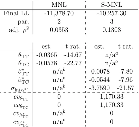
Table 1: Estimation results for empirical example: part I
MNL S-MNL Final LL -11,378.70 -10,257.30
par. 2 3
adj. ρ2 0.0353 0.1303
est. t-rat. est. t-rat.
θTT -0.0365 -14.67 n/aa
θTC -0.0578 -22.77 n/aa
β∗TT n/ab -0.0078 -7.80
β∗TC n/ab -0.0544 -7.96
σln(α∗) n/ab -3.7590 -21.57
cvθTT 0 1,170.33
cvθTC 0 1,170.33
cvβ∗TT n/ab 0
cvβ∗TC n/ab 0
a separate components estimated
b no separate components estimated
as S-MNL. In the MNL model, we estimate fixed time (θTT) and cost (θTC)
co-efficients. In the S-MNL model, we estimate separate β∗ and α∗ components, where the random scale parameterα∗ follows a lognormal distribution, i.e. using a normal distribution for ln (α∗). This specification ensures positive signs only, where the mean for the underlying normal distribution was set to zero for identi-fication (giving a median of 1 forα∗), withσln(α∗) giving the standard deviation
for the underlying normal distribution. No heterogeneity is estimated forθin the MNL model, and while we make a homogeneity assumption forβ∗ in the S-MNL model, the heterogeneity inα∗ leads to heterogeneity inθ in this model.
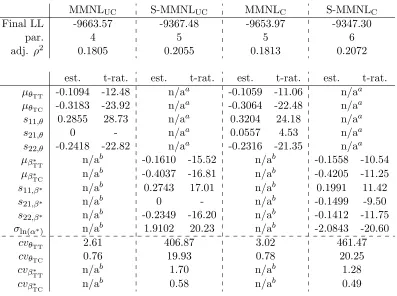
Table 2: Estimation results for empirical example: part II
MMNLUC S-MMNLUC MMNLC S-MMNLC
Final LL -9663.57 -9367.48 -9653.97 -9347.30
par. 4 5 5 6
adj. ρ2 0.1805 0.2055 0.1813 0.2072
est. t-rat. est. t-rat. est. t-rat. est. t-rat.
µθTT -0.1094 -12.48 n/a
a -0.1059 -11.06 n/aa
µθTC -0.3183 -23.92 n/a
a -0.3064 -22.48 n/aa
s11,θ 0.2855 28.73 n/aa 0.3204 24.18 n/aa
s21,θ 0 - n/aa 0.0557 4.53 n/aa
s22,θ -0.2418 -22.82 n/aa -0.2316 -21.35 n/aa
µβ∗
TT n/a
b -0.1610 -15.52 n/ab -0.1558 -10.54
µβ∗
TC n/a
b -0.4037 -16.81 n/ab -0.4205 -11.25
s11,β∗ n/ab 0.2743 17.01 n/ab 0.1991 11.42
s21,β∗ n/ab 0 - n/ab -0.1499 -9.50
s22,β∗ n/ab -0.2349 -16.20 n/ab -0.1412 -11.75
σln(α∗) n/ab 1.9102 20.23 n/ab -2.0843 -20.60
cvθTT 2.61 406.87 3.02 461.47
cvθTC 0.76 19.93 0.78 20.25
cvβ∗
TT n/a
b 1.70 n/ab 1.28
cvβ∗
TC n/a
b 0.58 n/ab 0.49
a separate components estimated
b no separate components estimated
excessively long tails obtained with this S-MNL model (see the coefficient of vari-ation for θ) are the result of this assumption; when imposing perfect correlation between coefficients, the true degree of heterogeneity is overstated. Finally, it is interesting to note a disproportionally large impact onβTT∗ in the S-MNL model, where the value of time drops from 37.91DKK/hr to just 8.65DKK/hr.
uncorrelated (UC) as well as correlated (C) specifications for the distribution of
θ, with the resulting models referred to as MMNLUC and MMNLC respectively.
We also estimate models which separate out α∗ and β∗, once again using a log-normal distribution forα∗, with models referred to as S-MMNLUC(uncorrelated)
and S-MMNLC (correlated) respectively.
The results for these models are summarised in Table 2. Looking at the notation for the MMNL models,µθTT and µθTC give the mean parameters, with
s11,θ and s22,θ giving the diagonal elements in the Cholesky matrix, and s21,θ
giving the off-diagonal element2. A corresponding notation is used in the other models.
The two MMNL models obtain highly significant gains in model fit over their MNL counterpart, with the same applying when comparing the two S-MMNL models to their S-MNL counterpart. Looking first at the models with uncor-related distributions, we see substantial gains in model fit for the S-MMNLUC
model over the MMNLUC model (296 units for one additional parameter) as a
result of separating out α∗. While the degree of heterogeneity in β∗ is lower in the S-MMNLUC model than was the case for the heterogeneity in θ in the
MMNLUC model, the overall heterogeneity in θ is increased substantially in the
S-MMNLUC model. This result is a reflection of the fact that the distribution
of θ = α∗β∗ in the S-MMNLUC model is different from that in the MMNLUC
model. This difference in flexibility also accounts for at least part of the gains in fit (and the split in heterogeneity between α∗ and β∗), making it impossible to make inferences about the retrieval of scale heterogeneity.
Using a correlated distribution forθTT andθTCin the MMNLCmodel leads to
a small but significant gain in fit (MMNLC vs. MMNLUC), while also suggesting
positive correlation between the two marginal utility coefficients (note that the product betweens11,θ and s21,θ is positive). This observation could be seen as a
direct result of this model capturing some of the scale heterogeneity in the data. Turning to the S-MMNLC model, we see that separate estimation of α∗ and β∗
once again leads to substantial gains in model fit (306.7 units for one additional parameter). Just as in the uncorrelated models, the degree of heterogeneity inβ∗
is lower in the S-MMNLC model than was the case for the heterogeneity inθ in
the MMNLC model, and we also note a reversal of the sign of the correlation in
that distribution. However, the heterogeneity in the overall distributionθis once again increased and the correlation between the elements in θ is again positive (noting thatσln(α) dominates in the covariance betweenθTT and θTC).
2
Withξ1andξ2being independent standard normal variates, draws from the distribution of
θTTare obtained asµθTT+s11(θ)ξ1, while draws from the distribution ofθTCare obtained as
µθTC+s21(θ)ξ1+s22(θ)ξ2. Correlation is allowed for asξ1 is used for both coefficients, with
In past work, the results from this example would have been used as evidence that a) there exists significant scale heterogeneity in the data, and b) the model at hand is able to disentangle the two components of heterogeneity. However, two issues arise. Firstly, the specification used for the distribution of the two marginal utility coefficients is inappropriate in the present context, as it would imply a substantial share of respondents with incorrectly signed time and cost coefficients. Secondly, the distribution used for θ = α∗β∗ in the S-MMNLUC
and S-MMNLC models is now a product between a lognormal distribution and
a normal distribution. The resulting distribution, known as the normal lognor-mal mixture (NLNM) distribution, is commonly used in the financial time series literature, and has well defined mathematical properties (see e.g. Clark, 1973;
Yang,2008). The NLNM distribution is more flexible than the typically assumed normal or lognormal distributions used when estimating MMNL models, in that the distribution (depending on the moments of the two underlying distributions) is non-symmetrical, being leptokurtic with negative skew, and not bounded at zero. From this perspective, the gains in fit (and the different patterns of hetero-geneity) obtained by incorporating a randomα are arguably at least in part due to this gain in flexibility. In the MMNLUC vs. S-MMNLUC comparison, the
ad-ditional issue arises that while the distribution ofθin the former is uncorrelated, the multiplication of uncorrelatedβ∗ distributions by a common α∗ distribution leads to correlation inθ=α∗β∗.
Informed by these discussions, we now make use of distributional assumptions that will a) ensure meaningful results from a micro-economic theory perspective and b) allow us to avoid issues with differences in flexibility between θ in the MMNL model andθ=α∗β∗in the S-MMNL model. This double aim is achieved by making use of a lognormal distribution for θ in the MMNL model, and log-normal distributions for both α∗ and β∗ in the S-MMNL model, ensuring that the resultingθ=α∗β∗ distribution will similarly be lognormal.
The results are summarised in Table 3, using much the same notation as before, where all estimates now relate to the normal distributions of the loga-rithms of coefficients. We once again see significant improvement of the MMNL and S-MMNL models over their MNL and S-MNL counterparts in Table1, while the fit (in terms of adjusted ρ2) is for each model also superior to that of the corresponding model from Table2.
In the discussion of these four models, we first focus on the two MMNL models. We see an improvement in model fit by 136 units for one additional parameter (the off-diagonal Cholesky term) when comparing MMNLC to MMNLUC. This
Table 3: Estimation results for empirical example: part III
MMNLUC S-MMNLUC MMNLC S-MMNLC
Final LL -9,462.84 -9,326.45 -9,326.70 -9,323.86
par. 4 5 5 6
adj. ρ2 0.1975 0.2090 0.2090 0.2092
est. t-rat. est. t-rat. est. t-rat. est. t-rat.
µln(θTT) -2.2203 -35.58 n/aa -1.7688 -26.81 n/aa
µln(θTC) -1.1830 -23.03 n/a
a -0.9430 -14.98 n/aa
s11,ln(θ) 1.1842 28.89 n/aa -1.8876 -18.99 n/aa
s21,ln(θ) 0 - n/aa -1.7371 -17.99 n/aa
s22,ln(θ) 1.6605 32.34 n/aa 1.5415 60.53 n/aa
µln(β∗
TT) n/a
b -1.7498 -27.54 n/ab -1.7353 -26.23
µln(β∗
TC) n/a
b -0.9205 -14.90 n/ab -0.9238 -13.95
s11,ln(β∗) n/ab 0.4127 19.49 n/ab 1.9004 18.91
s21,ln(β∗) n/ab 0 - n/ab 1.8105 18.44
s22,ln(β∗) n/ab 1.4721 63.32 n/ab 1.5296 49.52
σln(α∗) n/ab 1.8556 18.40 n/ab -0.1169 -0.37
cvθTT 1.75 6.01 5.85 6.04
cvθTC 3.84 16.50 14.80 16.67
cvβ∗
TT 1.75 0.43 5.85 6.00
cvβ∗
TC 3.84 2.78 14.80 16.56
a separate components estimated b no separate components estimated
increases in the degree of heterogeneity. This result is in line with the comparison between MMNLC to MMNLUC in the normal case (cf. Table 2).
We now proceed to the discussion of the two S-MMNL models. In both models, the coefficients used to multiply the attributes in the utility functions are given byθ = α∗β∗. The multiplication of two lognormals produces another lognormal distribution, where, independently of whether β∗ is uncorrelated or correlated, the resulting distribution forθ will be correlated. With the exception of MMNLUC, the various specifications in Table3are thus formally equivalent, as
multiple solutions fors11,ln(β∗),s21,ln(β∗),s22,ln(β∗)and σln(α∗) that give the same
covariance forθ, a conclusion that can be reached by noting that only three values are needed to specify the covariance matrix between two coefficients3. This issue
would always arise when the distribution of θ = α∗β∗ in a model of the type in Equation 3 is consistent with the distribution of a directly estimated θ in a model of the type in Equation 2. This point illustrates that when satisfying the condition that the distribution used for θ in the base model is of the same degree of flexibility as that used forθ =α∗β∗ in the S-MMNL model, efforts to disentangle scale heterogeneity from heterogeneity in relative sensitivities are in vain. Conversely, if the distribution for θ in the simple MMNL model differs in flexibility from that of θ =α∗β∗ in the S-MMNL model, it is impossible to say whether any gains in fit are the result of more flexible distributional assumptions or a sign of an ability to retrieve scale heterogeneity.
5
Summary and conclusions
There has been growing interest of late in the possibility that a large share of the heterogeneity retrieved in random coefficients models relates to variations in absolute sensitivities, i.e. scale heterogeneity, rather than variations in relative sensitivities.
This paper has not set out to discredit the possibility that scale heterogeneity across respondents exists. Our focus has rather been on attempts in the literature to disentangle the two components of heterogeneity, i.e. scale heterogeneity and heterogeneity in individual sensitivities. While the ability to separately identify the two components might be regarded as interesting from a behavioural analysis perspective, we argue that this is not in fact possible in a random heterogeneity context.
Our reasoning is based on two key principles. Firstly, an appropriately spec-ified “standard” Mixed Logit model, in particular one making use of correlated
3In the MMNL
C model, draws from θTT are obtained as e
µln(θ
TT)+s11,ln(θ)ξ1, with draws
from βTC being obtained as eµln(θTC)+s21,ln(θ)ξ1+s22,ln(θ)ξ2, with ξ1 and ξ2 once again giving
independent standard normal variates. In the S-MMNLC model, draws from α∗ are obtained
aseσln(α∗)ξ3, whereξ3 is an additional standard normal variate. The draws for θTT =α∗β∗
TT
are thus given bye
µ
ln(β∗TT)+s11,ln(β∗)ξ1+σln(α∗)ξ3
, while the draws for θTC = α∗βTC∗ are given
bye
µ
ln(βTC∗ )+s21,ln(β∗)ξ1+s22,ln(β∗)ξ2+σln(α∗)ξ3
. Working on the basis of the underlying normal distribution, we can see that the variance of ln (θTT) is equal to s11,ln(β∗)2 +σln(α∗)2, while,
for ln (θTC), the variance is given bys21,ln(β∗)2+s22,ln(β∗)2+σln(α∗)2. Finally, the covariance
between ln (θTT) and ln (θTC) is given bys21,ln(β∗)s11,ln(β∗)+σln(α∗)2. However, the exact same
covariance matrix can be obtained on the basis of a correlatedθalone, as in the MMNLCmodel,
distributions, is by definition capable of capturing scale heterogeneity alongside heterogeneity in individual coefficients. Secondly, attempts to disentangle the two have been based on making use of models where the marginal utility is given by a product of two random terms, one of which is shared across attributes. This specification leads to a more flexible distributional form, and any gains in fit may be the result of that flexibility in shape rather than an ability to capture scale heterogeneity. In summary, this means that while some of the heterogeneity cap-tured in the “scale” parameter in such models (α in our notation) may indeed relate to scale heterogeneity, there is no way for the analyst to determine whether that is indeed the case, or what share of the heterogeneity that may be.
The observations in this paper apply not just to work on random scale het-erogeneity, but also work on WTP space estimation. Such models differ from preference space models only in terms of the ease by which standard distributions can be used within each specification and how the parameters are interpreted. If a model estimated in WTP space fits better on a given data set, this is simply a reflection that the resulting distributional assumptions better match the data being modelled. The same argument applies to comparisons between say the G-MNL model and a model not attempting to include a multiplicative random term shared across coefficients. The G-MNL model (or any model multiplying two random parameters) simply has a greater candidate set of distributions for the marginal utility coefficients. That is to say that all such models are strictly nested and that what is being examined in such comparisons are simply alter-native distributional assumptions and the ease by which each parameterisation can accommodate the assumptions. This observation also relates to discussions inMcFadden and Train (2000).
As a direction for future research, we encourage analysts interested in scale heterogeneity to attempt to explain such heterogeneity through exogenous means (e.g. Caussade et al., 2005;Dellaert et al., 1999; Hensher et al., 1998; Louviere et al.,2000;Swait and Adamowicz,2001;Swait and Louviere,1993) or by mak-ing use of additional model components to quantify the role scale parameter (e.g.
6
Acknowledgements
The first author acknowledges the financial support by the Leverhulme Trust, in the form of a Leverhulme Early Career Fellowship. The majority of this work was carried out during a visit by the first author to the Institute of Transport and Logistics Studies at the University of Sydney, which was made possible by a Faculty of Economics and Business Visiting Scholar Grant. The authors would like to thank Kenneth Train and Thijs Dekker for valuable feedback on an earlier version of this paper.
References
Ben-Akiva, M., Lerman, S. R., 1985. Discrete Choice Analysis: Theory and Ap-plication to Travel Demand. MIT Press, Cambridge, MA.
Bhat, C. R., 2001. Quasi-random maximum simulated likelihood estimation of the mixed multinomial Logit model. Transportation Research Part B 35 (7), 677–693.
Breffle, W. S., Morey, E. R., 2000. Investigating preference heterogeneity in a repeated discrete-choice recreation demand model of atlantic salmon fishing. Marine Resource Economics 15, 1–20.
Brownstone, D., Bunch, D. S., Train, K., 2000. Joint Mixed Logit models of stated and revealed preferences for alternative-fuel vehicles. Transportation Research Part B 34 (5), 315–338.
Burge, P., Rohr, C., 2004. DATIV: SP Design: Proposed approach for pilot survey. Tetra-Plan in cooperation with RAND Europe and Gallup A/S.
Caussade, S., Ort´uzar, J. de D., Rizzi, L. I., Hensher, D. A., 2005. Assessing the influence of design dimensions on stated choice experiment estimates. Trans-portation Research Part B 39 (7), 621–640.
Clark, P. K., 1973. A subordinate stochastic process model with finite variance for speculative prices. Econometrica 41 (1), 135–155.
Daly, A., Hess, S., Train, K., 2011. Assuring finite moments for willingness to pay estimates from random coefficients models. Transportation forthcoming. Dellaert, B., Brazell, J. D., Louviere, J. J., 1999. The effect of attribute variation
Doornik, J. A., 2001. Ox: An Object-Oriented Matrix Language. Timberlake Consultants Press, London.
Fiebig, D. G., Keane, M., Louviere, J. J., Wasi, N., 2010. The generalized multino-mial logit: accounting for scale and coefficient heterogeneity. Marketing Science 29 (3), 393–421.
Fosgerau, M., Bierlaire, M., 2009. Discrete choice models with multiplicative error terms. Transportation Research Part B 43 (5), 494–505.
Greene, W. H., Hensher, D. A., 2010. Does scale heterogeneity across individuals matter? an empirical assessment of alternative logit models. Transportation 37 (3), 413–428.
Halton, J., 1960. On the efficiency of certain quasi-random sequences of points in evaluating multi-dimensional integrals. Numerische Mathematik 2 (1), 84–90.
Hensher, D. A., Greene, W. H., 2003. The Mixed Logit Model: The State of Practice. Transportation 30 (2), 133–176.
Hensher, D. A., Louviere, J. J., Swait, J., 1998. Combining sources of preference data. Journal of Econometrics 89 (1-2), 197–221.
Hess, S., Bierlaire, M., Polak, J. W., 2005. Estimation of value of travel-time savings using mixed logit models. Transportation Research Part A 39 (2-3), 221–236.
Hess, S., Rose, J. M., 2010. Random scale heterogeneity in discrete choice models. paper presented at the 89th Annual Meeting of the Transportation Research Board, Washington, D.C.
Hess, S., Stathopoulos, A., 2011. Linking response quality to survey engagement: a combined random scale and latent variable approach. ITS working paper. Institute for Transport Studies, University of Leeds.
Keane, M., 2006. The generalized logit model: preliminary ideas on a research program. presentation at Motorola-CenSoC Hong Kong meeting, October 22, 2006.
Louviere, J. J., Hensher, D. A., Meyer, R. J., Irwin, J., Bunch, D. S., Carson, R., Dellaert, B., Hanemann, W. M., 1999. Combining sources of preference data for modeling complex decision processes. Marketing Letters 10 (3), 205–217.
Louviere, J. J., Hensher, D. A., Swait, J., 2000. Stated Choice Models: Analysis and Application. Cambridge University Press, Cambridge.
Louviere, J. J., Islam, T., Wasi, N., Street, D., Burgess, L., 2008. Designing discrete choice experiments: Do optimal designs come at a price? Journal of Consumer Research 35, 360–375.
Louviere, J. J., Meyer, R. J., 2008. Formal choice models of informal choices: What choice modeling research can (and can’t) learn from behavioral theory. Review of Marketing Research 4, 3–32.
Louviere, J. J., Street, D., Carson, R., Ainslie, A., DeShazo, J. R., Cameron, T., Hensher, D. A., Kohn, R., Marley, T., 2002. Dissecting the random component of utility. Marketing Letters 13 (3), 177–193.
McFadden, D., Train, K., 2000. Mixed MNL Models for discrete response. Journal of Applied Econometrics 15 (5), 447–470.
Scarpa, R., Thiene, M., Train, K., 2008. Utility in Willingness to Pay Space: a tool to address the confounding random scale effects in destination choice to the alps. American Journal of Agricultural Economics 90 (4), 994–1010. Swait, J., 2006. Advanced choice models. In: Kanninen, B. (Ed.), Valuing
Envi-ronmental Amenities Using Stated Choice Studies: A Common Sense Approach to Theory and Practice. Springer, Dordrecht.
Swait, J., Adamowicz, W., 2001. Choice environment, market complexity, and consumer behavior: A theoretical and empirical approach for incorporating decision complexity into models of consumer choice. Organizational Behavior and Human Decision Processes 86 (2), 141–167.
Swait, J., Bernardino, A., 2000. Distinguishing taste variation from error struc-ture in discrete choice data. Transportation Research Part B 34 (1), 1–15. Swait, J., Louviere, J. J., 1993. The role of the scale parameter in the estimation
and comparison of multinomial logit models. Journal of Marketing Research 30 (3), 305–314.
Walker, J., 2001. Extended discrete choice models: Integrated framework, flexible error structures, and latent variables. Ph.D. thesis, MIT, Cambridge, MA.