Turbulent drag reduction through oscillating discs

This is a repository copy of

Turbulent drag reduction through oscillating discs

.

White Rose Research Online URL for this paper:

http://eprints.whiterose.ac.uk/137018/

Version: Accepted Version

Article:

Wise, D.J. and Ricco, P. orcid.org/0000-0003-1537-1667 (2014) Turbulent drag reduction

through oscillating discs. Journal of Fluid Mechanics, 746. pp. 536-564. ISSN 0022-1120

https://doi.org/10.1017/jfm.2014.122

eprints@whiterose.ac.uk https://eprints.whiterose.ac.uk/ Reuse

Items deposited in White Rose Research Online are protected by copyright, with all rights reserved unless indicated otherwise. They may be downloaded and/or printed for private study, or other acts as permitted by national copyright laws. The publisher or other rights holders may allow further reproduction and re-use of the full text version. This is indicated by the licence information on the White Rose Research Online record for the item.

Takedown

If you consider content in White Rose Research Online to be in breach of UK law, please notify us by

Turbulent drag reduction

through oscillating discs

Daniel J. Wise

_†

and Pierre Ricco

Department of Mechanical Engineering, The University of Sheffield, Mappin Street, S1 3JD Sheffield, United Kingdom

(Received 28 March 2014)

This article has been accepted for publication inJournal of Fluid Mechan-ics.

The changes of a turbulent channel flow subjected to sinusoidal oscillations of wall flush-mounted rigid discs are studied by means of direct numerical simulations. The Reynolds number is Rτ=180, based on the friction velocity of the stationary-wall case and the half channel height. The primary effect of the wall forcing is the sustained reduction of wall-shear stress, which reaches a maximum of 20%. A parametric study on the disc diameter, maximum tip velocity, and oscillation period is presented, with the aim to identify the optimal parameters which guarantee maximum drag reduction and maximum net energy saving, the latter computed by taking into account the power spent to actuate the discs. This may be positive and reaches 6%.

The Rosenblat viscous pump flow, namely the laminar flow induced by sinusoidal in-plane oscillations of an infinite disc beneath a quiescent fluid, is used to predict accurately the power spent for disc motion in the fully-developed turbulent channel flow case and to estimate localized and transient regions over the disc surface subjected to the turbulent regenerative braking effect, for which the wall turbulence exerts work on the discs.

The Fukagata-Iwamoto-Kasagi identity is employed effectively to show that the wall-friction reduction is due to two distinguished effects. One effect is linked to the direct shearing action of the near-wall oscillating disc boundary layer on the wall turbulence, which causes the attenuation of the turbulent Reynolds stresses. The other effect is due the additional disc-flow Reynolds stresses produced by the streamwise-elongated structures which form between discs and modulate slowly in time.

The contribution to drag reduction due to turbulent Reynolds stress attenuation de-pends on the penetration thickness of the disc-flow boundary layer, while the contribution due to the elongated structures scales linearly with a simple function of the maximum tip velocity and oscillation period for the largest disc diameter tested, a result suggested by the Rosenblat flow solution. A brief discussion on the future applicability of the oscillating-disc technique is also presented.

Key words:

1. Introduction

Significant effort in the fluid mechanics research community is currently directed to-wards turbulent drag reduction, motivated by the possibility of huge economic savings in

many industrial scenarios. The necessity for improved environmental sustainability has spurred vast academic and industrial interest in the development of novel drag-reduction techniques and in understanding the underlying physical mechanisms. Although to date there exist many control strategies for drag reduction, notably MEMS-based closed-loop feedback control (Kasagiet al.2009) and open-loop large-scale wall-forcing control (Jung

et al. 1992; Berger et al. 2000; Quadrio & Sibilla 2000), none have been implemented in industrial systems. Amongst the open-loop active drag reduction methods, for which energy is fed into the system in a pre-determined manner, particular attention has been devoted to those which employ in-plane wall motion. A recent review is found in Quadrio (2011) and a brief discussion is presented in the following.

1.1. The oscillating wall

The direct numerical simulations by Junget al.(1992) and the experimental campaign by Laadhariet al. (1994) of turbulent wall-bounded flows subjected to sinusoidal spanwise wall oscillations produced a rich vein of work in this area. Their findings first revealed the ability of the actuated wall to suppress the frequency and intensity of near-wall turbulent bursts and to yield a maximum sustained wall friction reduction of about 45%. The existence of an optimal oscillation period for fixed maximum wall velocity,T+ _≈120

(where + indicates scaling in viscous units with respect to the uncontrolled case) has been widely documented (Quadrio & Ricco 2004). It was recognized by Choiet al.(2002) that the space-averaged turbulent spanwise flow agrees closely with the laminar solution to the Stokes second problem for oscillation periods smaller or comparable with the optimum one, which led to the use of a scaling parameter for the drag reduction. Quadrio & Ricco (2004) found a linear relation between this parameter - a measure of the penetration depth and acceleration of the Stokes layer - and the drag reduction, noted to be valid only forT+ _{6150. Quadrio & Ricco (2004) were also the first to explain the existence}

of the optimum period by comparing it with the characteristic Lagrangian survival time of the near-wall turbulent structures. More recently, Ricco et al. (2012) endowed the scaling parameter with a more direct physical meaning, showing it to be proportional to the maximum streamwise vorticity created by the Stokes layer at constant maximum velocity. Through an analysis of the turbulent enstrophy balance, Ricco et al. (2012) were also able to identify the key production term in the turbulent enstrophy equation, which is balanced by the change in turbulent dissipation near the wall. More importantly, by studying the transient evolution from the start-up of the wall motion, they showed that the turbulent kinetic energy and the skin-friction coefficient decrease because of the short-time transient increase of turbulent enstrophy. This is the latest effort aimed at elucidating the drag reduction mechanism, after research works based on the disruption of the near-wall coherent structures (Baron & Quadrio 1996), the cyclic inclination of the low-speed streaks (Bandyopadhyay 2006), the weakening of the low-speed streaks (Di Ciccaet al.2002; Iusoet al.2003), and simplified models of the turbulence-producing cycle (Dhanak & Si 1999; Moarref & Jovanovic 2012; Duque-Dazaet al. 2012).

1.2. The wall waves

Skote (2013) also showed that the damping of the turbulent Reynolds stresses depends on the penetration depth of the spatial Stokes layer.

The oscillating-wall and the steady-wave techniques were generalized by Quadrioet al.

(2009) by considering wall turbulence forced by wall waves of spanwise velocity of the formWf=Wcos [2π(x/λx−t/T)]. A maximum drag reduction of 47% and a maximum net energy saving of 26% were computed. For wall waves travelling at a phase speed comparable with the near-wall turbulent convection velocity, drag increase was also found. Despite the widespread interest in turbulent drag reduction by active wall forcing, the implementation of these techniques in industrial settings appears to be an insurmount-able challenge. Progress is nonetheless being made to improve this scenario. Prominent amongst recent efforts is the experimental work by Gouder et al. (2013) on in-plane forcing of wall turbulence through a flexible wall made of electroactive polymers. The main reasons which render the technological applications of active techniques an involved engineering task arei)the extremely small typical time scale of the wall forcing (the op-timal period for the oscillating-wall technique translates to a frequency of 15,000Hz in commercial aircraft flight conditions), and ii) the requirement of large portion of the surface to be in uniform motion. Therefore, drag reduction methods which operate on a large time scale and rely on finite-size wall actuation are preferable in view of future applications.

1.3. The rotating discs

The novel actuation strategy based on flush-mounted discs rotating upon detection of the bursting process, first proposed by Keefe (1998), undoubtedly belongs to a group of inter-esting control methods which employ finite-size actuators. However, Keefe did not follow up on his innovative idea and neither experimental nor numerical results appeared in the subsequent 15 years. Ricco & Hahn (2013) (denoted by RH13 hereafter) showed revived interest in this flow and investigated an open-loop variant of Keefe’s technique whereby the discs rotate with a pre-determined constant angular velocity. A numerical parametric investigation onD, the disc diameter, and W, the disc tip velocity, yielded maximum values for drag reduction and net power saved of 23% and 10%, respectively. RH13 also showed that drag increase occurs for small diameter and small rotational periods, that the disc-flow boundary layer must be thicker than a threshold to obtain drag reduction, and that the power spent to activate the discs can be calculated accurately through the von K´arm´an laminar viscous pump solution (Panton 1995) under specified conditions. The Fukagata-Iwamoto-Kasagi (FIK) identity (Fukagata et al. 2002) was modified for the disc flow to show that the near-wall streamwise-elongated jets appearing between discs provide a favourable contribution to drag reduction. Promisingly, the optimal spa-tial and temporal scales were L+ _{= O(1000) and T}+ _{= O(500). This is a significant}

result when these scales are compared with those of other localized actuation strategies, such as the feedback control based on wall transpiration (Yoshinoet al.2008), which are thought to operate optimally at spatio-temporal scalesL+ _{=O(30) andT}+ _=O(100).

It is our hope that the results of RH13 will therefore offer fertile ground for new avenues of future research on active turbulent drag reduction.

1.4. Objectives and structure of the paper

budget, computed by taking into account the power spent to activate the discs. The laminar solution for the flow over an oscillating disc proves useful to estimate the power spent to activate the discs, to predict the occurrence of regenerative braking effect, and to define scaling parameters for drag reduction. An analogy is also drawn to the oscillating wall technique to discuss the drag reduction mechanism at work in the oscillating-disc flow.

The numerical procedures, flow field decompositions and performance quantities are described in §2. The solution of the laminar flow is presented in §3, where it is used to compute the power spent to move the discs and to predict the regenerative braking effect. The turbulent flow results are presented in §4. The dependence of drag reduction on the disc parameters is discussed in §4.1 and §4.2. In section §4.3 the FIK identity is modified to account for the disc flow effects, while §4.4 presents visualisations and statistics of the disc flow. Section §4.5 includes a comparison between the turbulent power spent and the corresponding laminar prediction. A discussion on the drag reduction physics and scaling is found in §4.6. Finally, section §5 presents an evaluation of the applicability of the technique to flows of technological interest, provides a guidance for future experimental studies, and offers a comparison with other drag reduction techniques, with particular focus on the typical length and time scales.

2. Flow definition and numerical procedures

2.1. Numerical solver, geometry and scaling

The simulated pressure-driven turbulent channel flow at constant mass flow rate is con-fined between two infinite parallel flat walls separated by a distanceL∗

y= 2h∗, where the symbol∗_{henceforth denotes a dimensional quantity. The streamwise pressure gradient is}

indicated by Π∗_{. The direct numerical simulation (DNS) code solves the incompressible}

Navier-Stokes equations in the channel flow geometry using Fourier series expansions along the streamwise (˜x∗_{) and spanwise (˜z}∗_{) directions, and Chebyshev polynomials}

along the wall-normal directiony∗_{. The time-stepping scheme is based on a third-order}

semi-implicit backward differentiation scheme (SBDF3), treating the nonlinear terms explicitly and the linear terms implicitly. The discretized equations are solved using the Kleiser-Schumann algorithm (Kleiser & Schumann 1980), outlined in Canutoet al.

(2007). Dealiasing is performed at each time step by setting to zero the upper third of the Fourier coefficients along the streamwise and spanwise directions. The simulations were carried out using an OpenMP parallel implementation of the code on the N8 HPC Polaris cluster. The code was also used by RH13 and it is a developed version of the original open-source code available on the Internet (Gibson 2006).

Lengths are scaled withh∗ _{and velocities are scaled withU}∗

p, the centreline velocity of the laminar Poiseuille flow at the same mass flow rate. The time is scaled byh∗

/U∗

p and the pressure byρ∗

U∗2

p , whereρ ∗

is the density of the fluid. The Reynolds number isRp=

U∗

ph ∗

/ν∗

= 4200, where ν∗

is the kinematic viscosity of the fluid. The friction Reynolds number is Reτ = u∗τh

∗

/ν∗

= 180, where u∗ τ =

p

τ∗

w/ρ∗ is the friction velocity in the stationary wall case, andτ∗

wis the space- and time-averaged wall-shear stress. Quantities non-dimensionalized using outer units are not marked by any symbol. Unless otherwise stated, the superscript + indicates scaling by native viscous units, a terminology first defined by Trujilloet al.(1997), based onu∗

τ of the case under investigation.

Lx

Lz

Ly

Mean flow ˜

x

˜ x ˜

z

˜ z y

D

f

W =Wcos(2πt/T)

Figure 1: Schematic of the flow domain showing the location and sense of rotation of the discs whenfW =W.

figure 1. The discs have diameterD and oscillate in time as the disc tip velocity is

f

W =Wcos

_2πt

T

. (2.1)

Neighbouring discs in the streamwise direction have opposing sense of rotation, whilst neighbouring discs in the spanwise direction have the same sense of rotation. A parametric study was undertaken on D, W and T, with the parameter range selected in order to focus on the portion of D, W parameter space studied by RH13 which leads to high drag reduction. The region of drag increase found by RH13 was not considered. For disc diametersD = 1.78,3.38, a computational box size of dimensionsLx = 6.79π and Lz = 2.26π was utilized, where Lx and Lz are the box lengths along the streamwise and spanwise directions, respectively. For D = 5.07, Lx = 6.8π and Lz = 3.4π, and for D = 6.76, Lx = 9.05π and Lz = 2.26π. The grid sizes were ∆x+ = 10, ∆z+ = 5 in all cases, and the time step was within the range 0.008 6 ∆t+ _{6 0.08 (scaled in}

reference outer units). The initial transient period during which the flow adjusts to the new oscillating-disc regime was discarded following the procedure outlined in Quadrio & Ricco (2004). Flow fields were saved over an integer number of periods at intervals of T /8. After the transient was discarded, the total integration time was t+_{=6000 for}

T+_{= 100,t}+_{=7500 for T}+_{= 250,500,t}+_{=15000 forT}+_{= 1000 andt}+_=30000.

2.2. Model of disc annular gap

r2

r1

uθ(r, t)

r θ

Figure 2: Schematic of disc and annular gap flow.

turbulent channel flow and gap flow as coupled systems, but this lies outside the scope of the present study.

As a first approximation, the gap velocity profile is assumed to be symmetric about the disc axis and to change linearly from a maximum velocity at the disc tip to zero at the outer edge of the gap. The tangential velocity uθ in this region is a function only ofr, the radial displacement from the centre of the disc, and time,t. The disc velocity profile is

uθ(r, t) =

2W rcos(2πt/T)/D, r6r1,

W(c−r+D/2) cos(2πt/T)/c, r16r6r2,

where r1 =D/2 and r2 =D/2 +c. As a more advanced approximation, the clearance

flow is modelled as a thin layer of fluid confined between concentric cylinders. Similarly to the laminar flow between moving flat plates, the flow contained within this annular gap is described by the Womersley number, Nw = c∗

p

2π/(ν∗_T∗_{) (Pozrikidis 2009).}

When Nw ≪ 1, the linear velocity profile accurately describes the flow. However, for Nw =O(1) the oscillating flow surrounding each disc is confined to a boundary layer which is attached to the oscillating disc and is much thinner than c. The bulk of the annular gap is quasi-stationary. In our simulations the minimum Nw = 0.51 occurs for the case with the thinnest gap and the largest oscillation period, i.e. for D = 1.78,

T = 130. The maximum Nw = 6.42 occurs for D = 7.1, T = 13. Therefore, it is a sensible choice to simulate the gap via the oscillating layer asNw attains finite values. Following the analysis of Carmi & Tustaniwskyj (1981), the uθ(r, t) velocity profile in the gap is described by the azimuthal momentum equation,

∂uθ

∂t =

1

Rp

∂2_u

θ

∂r2 +

1

r

∂uθ

∂r −

uθ

r2

. (2.2)

Assuming a solution to (2.2) of the formuθ=R

h

˚uθ(r)ei2πˆt/T

i

, whereRdenotes the real part and ˆtis the rescaled time, ˆt=t/Rp, the following ordinary differential equation of the Bessel type is obtained

˚u′′ θ+

˚u′ θ

r −

2πi

T +

1

r2

˚uθ= 0, (2.3)

-12 -6 0 6 12 620

625 630 635 640

r

+

u+

θ

-12 -6 0 6 12

620 625 630 635 640

r

+

u+

θ

Figure 3: Velocity profiles within the annular gap over a half period of the oscillation, computed through (2.4). Left:D= 7.1,W = 0.51,T = 130,Nw= 2.03. Right: D= 7.1, W = 0.51,T = 13,Nw= 6.42.

˚uθ(r1) =W, ˚uθ(r2) = 0. The velocity in the annular gap is

uθ(r,ˆt) =W ·R

K(ξr2)I(ξr)− I(ξr2)K(ξr)

I(ξr1)K(ξr2)− I(ξr2)K(ξr1)

ei2πˆt/T

, (2.4)

whereI(·) andK(·) are the first-order modified hyperbolic Bessel functions (Abramowitz & Stegun 1964) andξ=pi2π/T. Velocity profiles are shown in figure 3. The Bessel layer was included in the code by reading in a map of the wall complex velocity at t= 0. To advance in time the components within this map were multiplied by e2πit/Tˆ _{and the}

real components were extracted. As the boundary conditions are implemented in spec-tral space, it was necessary to Fourier transform the time-updated map of the velocity components at each time step, before passing the Fourier components as boundary con-ditions.

The difference between the values of drag reduction and power spent against the viscous forces computed by use of the two annular-gap models for c = 0,0.02D, and 0.05D

were within the uncertainty range estimated via numerical resolution checks based on variation of the mesh sizes, time step advancement, and size of the computational box (refer to RH13 for further details on the numerical resolution tests). For this reason and because of the higher computational cost caused by the Bessel profile due to the additional spectral transformations, the linear velocity profile model was used. In order to choose the appropriate gap size for the simulations, the dimensional gap values were examined for typical experimental scenarios, presented in table 6 of RH13 for the steady disc flow case. The largest tested gap size ofc= 0.05Dwas implemented as it corresponds to a value that would be achievable in the laboratory conditions detailed in this table.

2.3. Flow decomposition

The averaging operators used to decompose the flow are defined in the following. The space- and time-ensemble average is defined as

f(x, y, z, τ) = 1

NxNzN

NXx−1

nx=0 NXz−1

nz=0 N_X−1

nt=0

where 2NxandNzare the number of discs within the computational domain along ˜xand ˜

z, respectively,τ is the window time of the oscillation, andN is the number of oscillation periods. The time average and the spatial average along the homogeneous directions are defined respectively as

hfi(x, y, z) = 1

T

Z T

0

f(x, y, z, τ)dτ, fˆ(y) = 1

LxLz

Z Lx

0 Z Lz

0 h

fi(x, y, z)dzdx. (2.6)

A global variable is defined as

[f]_g=

Z 1

0

ˆ

f(y)dy.

The size of all statistical samples is doubled by averaging over the two halves of the channel, taking into account the existing symmetries. The channel flow field is expressed by the sum

u(x, y, z, t) =um(y) +ud(x, y, z, τ) +ut(x, y, z, t), (2.7)

where um(y) ={u_m,0,0}= ˆuis the mean flow,ud(x, y, z, τ) = {u_d, v_d, w_d}=u−um is the disc flow, andut is the fluctuating turbulent component.

2.4. Performance quantities

This section introduces the main quantities used to describe the oscillating-disc flow, i.e. the turbulent drag reduction, the power spent to activate the discs against the viscous resistance of the fluid, and the net power saved, which is their algebraic sum.

2.4.1. Turbulent drag reduction

The skin-friction coefficientCfis first defined asCf=2τw∗/ ρ ∗

U∗2

b

, whereU∗ b=[u

∗

]g/h∗ is the bulk velocity. The latter is constant because the simulations are performed under conditions of constant mass flow rate. The drag reductionRis defined as the percentage change of the skin-friction coefficient with respect to the stationary wall value (Quadrio & Ricco 2004):

R(%) = 100Cf,s−Cf

Cf,s

, (2.8)

where the subscriptsrefers to the stationary wall case. Usingτ∗ w=µ

∗

u∗′

m(0), where the prime denotes differentiation with respect toy, (2.8) becomesR(%) = 100· 1−u′

m(0)/u ′ m,s(0)

.

2.4.2. Power spent

As the oscillating disc flow is an active drag reduction technique, power is supplied to the system to move the discs against the viscous resistance of the fluid. To calculate the power spent, term III of the instantaneous energy equation (1-108) in Hinze (1975) is first considered. Its volume-average is the work done by the viscous stresses per unit time,

P∗ sp,t=

ν∗

L∗

xL∗yL∗z

Z L∗ x

0 Z L∗

y

0 Z L∗

z 0 ∂ ∂x∗ i " u∗ j ∂u∗ i ∂x∗ j +∂u ∗ j ∂x∗ i !#

d˜z∗

dy∗

d˜x∗

, (2.9)

wherei, jare the indexes indicating the spatial coordinates ˜x,y, ˜zand the corresponding velocity components (Einstein summation of repeated indexes is used). By substituting (2.7) into (2.9) and by use of (2.5) and (2.6), one finds

P∗ sp,t=

ν∗

h∗

 u\∗

d ∂u∗ d ∂y∗ _y∗₌₀

+w\∗ d ∂w∗ d ∂y∗ _y∗₌₀



The power spent (2.10) is expressed as percentage of the power employed to drive the fluid in the streamwise direction,P∗

x. By volume-, ensemble- and time-averaging the first term on the right-hand side of (1-108) in Hinze (1975), one obtains

P∗ x=

U∗

bΠ ∗

ρ∗ , (2.11)

By dividing (2.10) by (2.11), the percentage power employed to oscillate the discs with respect to the power spent to drive the fluid along the streamwise direction is obtained,

Psp,t(%) =− 100Rp

R2

τUb

 u\d

∂ud

∂y

y=0

+w\d

∂wd

∂y

y=0 

. (2.12)

2.4.3. Net power saved

The net power saved, Pnet, the difference between the power saved due to the disc forcing (which coincides with Rfor constant mass flow rate conditions) and the power spentPsp,t, is defined as

Pnet(%) =R(%)− Psp,t(%). (2.13)

3. Laminar flow

For other active turbulent drag reduction techniques the analytical solutions for the corresponding laminar flows induced by wall motion have proven useful for accurately estimating important averaged turbulent quantities, such as the wall spanwise shear (Choiet al.2002), the power spent for the wall forcing (Ricco & Quadrio 2008), and the thickness of the generalized Stokes layer generated by the wall waves (Skote 2011). The laminar solution has also been employed to determine a scaling parameter which relates uniquely to drag reduction under specified wall forcing conditions (Quadrio & Ricco 2004; Cimarelli et al. 2013). Through the laminar solution of the flow induced by a steadily rotating infinite disc, RH13 obtained an estimate of the time-averaged power spent to move the discs, which showed very good agreement with the power spent computed via DNS.

Inspired by previous works, the laminar flow above an infinite oscillating disc is there-fore computed to calculate the power spent to activate the disc and to identify areas over the disc surface where the fluid performs work onto the discs, thus aiding the rota-tion. This is a form of the regenerative braking effect, studied by RH13 for steady disc rotation. These estimates are then compared with the turbulent quantities in §4.5.

3.1. Laminar flow over an infinite oscillating disc

The laminar oscillating-disc flow was studied for the first time by Rosenblat (1959) (refer to figure 2 for the flow geometry). The velocity components are

{u∗ r, u

∗ θ}=

2r∗

W∗

D∗

F′

η,˘t, G η,˘t , u∗

y=− 4W∗

D∗

r

ν∗_T∗

π F η,t˘

, (3.1)

where the prime denotes differentiation with respect to η = y∗p_π/(ν∗_T∗_{), the scaled}

wall-normal coordinate, ˘t = 2πt∗_/T∗ _{is the scaled time, and u}∗

r, u∗θ and u ∗

conditions are satisfied

y∗

= 0 : u∗

r= 0, u ∗ θ= (2r

∗

W∗

/D∗

) cos ˘t, u∗

y= 0, p ∗

= 0.

y∗

→ ∞: u∗

r= 0, u ∗ θ= 0.

Expressions (3.1) are substituted into the cylindrical Navier-Stokes equations to obtain the equations of motion forF′ _{andGunder the boundary layer approximation,}

˙

F′₌ 1

2F

′′′

+γ(G2+ 2F F′′

−F′2_),

˙

G= 1

2G

′′

+ 2γ(F G′ −F′

G),

(3.2)

with boundary conditions

η= 0 : F=F′_{= 0, G= cos ˘t,}

η→ ∞: F′ _{=G= 0,} (3.3)

where the dot denotes differentiation with respect to ˘t and γ = T∗

W∗

/(πD∗

). The latter parameter represents the ratio between the oscillation periodT∗

and the period of rotation πD∗

/W∗

which would occur if the disc rotated steadily with tip velocityW∗

. The value γ = π is relevant because it denotes the special case of maximum disc tip displacement equal to the circumference of the disc, i.e. each point at the disc tip covers a distance equal toπD∗

during a half period of oscillation.

The system (3.2)-(3.3) was discretized using a first-order finite difference scheme for ˘t

and a second-order central finite difference scheme forη. The equations were first solved in time by starting from null initial profiles. The boundary condition forGwas altered as

G 0,˘t= 1−e−˘t_{untilGwas sufficiently close to unity. The system was then integrated} with the boundary conditionG 0,˘t= cos ˘t. Figure 4 (left) shows the wall-normal profiles ofF′ _{andGat different oscillation phases.}

3.2. Laminar power spent

The laminar power spent P∗

sp,l is calculated using (2.9), where only ud is retained in the laminar case as there is no mean streamwise flow above the disc and the turbulent fluctuations are null (um =ut = 0). Substitutingud =uθcosθ andwd =uθsinθ into (2.9), using (3.1) and averaging overθ,r, and time leads to

P∗ sp,l= G

(γ)W∗2

2

r

πν∗

T∗ , (3.4)

where

G(γ) = 1 2π

Z 2π

0

G 0,˘tG′

0,˘td˘t (3.5)

is shown in figure 4 (right). To expressP∗

sp,l as percentage of the power spent to drive the fluid along the streamwise direction, (3.4) is divided by (2.11) to obtain

Psp,l(%) =

50G(γ)W2_R3/2

p

UbR2τ

r

π

T. (3.6)

3.2.1. Asymptotic limit for γ≪1: the Stokes-layer regime

To obtain an analytical approximation to G for γ ≪ 1, the expanded form of G in powers ofγ can be used,

0 0.05 0.1 0

0.5 1 1.5 2 2.5 3

η

F′

-0.5 0 0.5 1 0

0.5 1 1.5 2 2.5 3

G

10 15 20 25 30 -2.5

-2 -1.5

0 2 4 6

-0.9 -0.8 -0.7 -0.6 -0.5 -0.4

G

G

γ

γ

Figure 4: Left: Wall-normal profiles ofF′ _{andGat different oscillation phases forγ= 1}

(thick lines) and γ= 0 (thin lines). The latter is given by (3.9) and coincides with the classical Stokes layer solution. Right: Numerically computed values ofG(γ) (solid lines) and asymptotic solutions, (3.8) forγ≪1 (dashed line in main plot), and (3.12) forγ≫1 (dashed line in inset).

whereG0andG2are given in equations (17) and (45) of Rosenblat (1959). Upon

differ-entiation of (3.7) with respect toη, the asymptotic form ofG(γ) is

Gγ≪1(γ) = 1

2π

Z 2π

0

G0(0,˘t)G′0(0,˘t) +γ2G

′

2(0,t˘)

d˘t=−1₂+ γ

2

160

15√2−26+O(γ3), (3.8) which is shown in figure 4 (right). The asymptotic solution predicts the numerical solution well forγ <2.

In the limitγ≪1, Rosenblat (1959) obtained a first-order solution

u∗

θ= 2r∗_W∗

D∗ e

−√π/(ν∗_T∗_)y∗

cos

_2πt∗

T∗ −

r

π

ν∗_T∗y

∗

, (3.9)

which is in the same form as the classical Stokes solution (Batchelor 1967). Substituting (3.9) into (2.9), the first-order approximation is found,P∗

sp,l= 0.25W ∗p

πν∗_/T∗_{, which}

is expressed as percentage of (2.11) to obtain

Psp,l,γ≪1=−

25W2_R3/2

p

UbRτ2

r

π

T. (3.10)

This is also found directly from (3.6) by settingG(0) =−0.5. 3.2.2. Asymptotic limit for γ≫1: the quasi-steady regime

As suggested by Benney (1964), in the limitγ ≫ 1 it is more appropriate to rescale the wall-normal coordinate by the Ekman layer thickness δ∗

e =

p

ν∗_D∗_/(2W∗_{). The}

rescaled equations (2.19) and (2.20) of Benney (1964) were then solved using the same numerical method described in §3.1. The von K´arm´an equations describing the flow over a steadily rotating disc are recovered in the limitγ→ ∞. The asymptotic limit ofG for

γ≫1 is found by first rescalingG′_{(0,˘t) in (3.5) throughδ}∗

modulation of the disc motion enters the problem only parametrically,

G′

γ≫1(0,˘t) = p

2γGscos ˘t, (3.11)

whereGs=−0.61592 (Rogers & Lance 1960). By substituting (3.11) into (3.5) and by use of (3.3), one finds

Gγ≫1(γ) =Gs

r

γ

2. (3.12)

As shown in figure 4 (right, inset), the asymptotic expression (3.12) matches the numeri-cal values well. By substituting (3.12) into (3.6), the asymptotic form of the power spent is obtained

Psp,l,γ≫1= 50GsW 3/2_R3/2

p √

2DUbRτ2

. (3.13)

By coincidence, the power spent whenγ= 0, i.e. (3.10), is half of the oscillating-wall case at the sameW∗

andT∗

(Ricco & Quadrio 2008), and the power spent whenγ≫1, i.e. (3.13), is half of the steady-rotation case at the sameW∗

andD∗

(RH13). The oscillating-disc power spent is expected to be smaller than in these two cases, but for different reasons. The oscillating-wall case requires more power because the motion involves the entire wall surface, while the steady-rotation case consumes more power because the motion is uniform in time.

3.3. Laminar regenerative braking effect

The laminar phase- and time-averaged power spentWl to oscillate the discs beneath a uniform streamwise flow is computed by following RH13. As the purpose of this analysis is to obtain a simple estimate of the turbulent case, the streamwise shear flow is superim-posed on the Rosenblat flow without considering their nonlinear interaction. A rigorous study of this flow would be the extension of the work by Wang (1989) with oscillatory wall boundary conditions. Starting from (2.9), using (2.7), and settingut= 0, one finds

Wl(x,0, z,˘t) = 1

Rp

"

ud(x,0, z,˘t) u′m(0) +

∂ud

∂y

_y=0

!

+wd(x,0, z,˘t)

∂wd

∂y

_y=0

#

.

(3.14) Using (3.1), (3.14) becomes

Wl(r,˘t) =

2rW G(0,˘t, γ)

DRp

u′

m(0) cosθ+ 2W r

D

r

πRp

T G

′

(0,˘t, γ)

!

.

By rearranging to obtain an inequality inr, the region where the streamwise flow exerts work on the disc (regenerative braking effect) is found,

r <−u

′

m(0)Dcosθ 2W G′_(0,˘_{t, γ)}

s

T

πRp

. (3.15)

In §4.5, the region of regenerative braking effect is computed for the turbulent case and compared with the laminar prediction (3.15).

4. Turbulent flow

1000 2000 3000 4000 0.00075

0.001 0.00125

t+

2

\∂u

/

∂

y

/ 0

(

U

2R_b

p

)

Fixed wall

W+ = 9.9,T+ = 833,R= 16.0% W+ = 9.8,T+ = 209,R= 15.8% W+ = 6.2,T+ = 95,R= 4.1%

0 200 400 600 800

0.0009 0.001 0.0011 0.0012

τ+

0 π 4

π 2

3π 4

π

5π 4

3π 2 7π

4

e

W

0 W

−W

Figure 5: Left: Space-averaged streamwise wall-shear stress vs. time for cases atD= 3.38. The disc forcing is initiated att+ _{= 770. Only a fraction of the total integration time}

is shown. The space-averaging operator here does not include time averaging. Right: Ensemble- and space-averaged streamwise wall-shear stress vs.τ+ _forD+_{= 554,W}+₌

9.9,T+_{= 833 (dashed line). The disc velocity is shown by the solid line. The phaseφis}

given in the figure.

and section §4.5 describes the power spent to move the discs and the comparison with the laminar prediction, studied in §3.2.

4.1. Time evolution

The temporal evolution of the space-averaged wall-shear stress is displayed in figure 5 (left). The transient time occurring between the start-up of the disc forcing and the fully established disc-altered regime increases withR. This agrees with the oscillating wall and RH13, but the duration of the transient for the discs is shorter than for the oscillating wall case. The time modulation of the wall-shear stress is notable for the highRcases, with the amplitude of the signal increasing withT. The significant time modulation and the shorter transient compared with the oscillating wall technique could be due to the discs forcing the wall turbulence in the streamwise direction. The streamwise wall-shear stress is therefore affected directly whereas in the oscillating-wall case the streamwise shear flow is modified indirectly as the motion is along the spanwise direction only.

The space- and phase-averaged wall-shear stress modulation, shown by the dashed line in figure 5 (right), has a period equal to half of the wall velocity. This is expected because of symmetry of the unsteady forcing with respect to the streamwise direction. The wall-shear stress reaches its minimum value approximatelyT /8 after the disc velocity is maximum, i.e. atφ= 5π/8,13π/8. The wall-shear stress peaks approximatelyT /8 after the disc velocity is null, i.e. atφ=π/8,9π/8.

4.2. Dependence of drag reduction on D,W,T

Figure 6 depicts maps ofR(T, W)(%) for disc sizesD= 1.78, 3.38, 5.07, and 6.76. Theγ

defined in (2.13). Only positivePnet values are shown and the bold boxes highlight the maximumPnetvalues.

For D = 1.78 and 3.38 and fixed W, drag reduction increases up to an optimum T

beyond which it decays. This optimum T depends on D, and increases with the disc diameter. ForD = 1.78,3.38 the optimal periods are in the rangesT+_{= 200−400 and}

T+_{= 400−800, respectively. ForD= 5.07 and 6.76 the optimal period is not computed}

and thereforeR increases monotonically withT for fixedW and D. Cases with larger

T are not investigated due to the increased simulation time required for the averaging procedure.

ForD = 1.78 and fixedT, drag reduction increases up to an optimum wall velocity,

W ≈0.26 (W+_{≈6), above which drag reduction decreases. This behaviour also occurs}

in the steady-disc case studied by RH13. The optimalW are not found for largerD as the drag reduction increases monotonically withW for fixedDandT.

For T ≫ 1, the wall forcing is quasi-steady and it is therefore worth comparing the

R value with the ones obtained by steady disc rotation, computed by RH13. RH13’s values are however not expected to be recovered in this limit. A primary reason for this is that the power spent in the oscillating-disc case is smaller than in the steady rotation case, as verified in §4.5 (in §3.2.2, it is predicted to be half of the steady case by use of the laminar solution when the oscillation period is large). RH13’s values are displayed in figure 7 by the dark grey circles on the right-hand side of each map. In most of the cases where the optimal T+ _{is detected, i.e. for W}+ _{> 3,D = 1.78, and for W}+ _>9,

D= 3.38 and 5.07, ourRvalues may reach larger values than RH13’s for the sameW+_.

ForD= 6.76, all our computedRare lower than RH13’s.

Figure 7 also shows that a positive Pnet occurs only for W+ 69. This confirms the finding by RH13 for steady rotation and is expected because the power spent grows rapidly asW grows, as also suggested by the laminar result in (3.6). The largest positive

Pnet in the parameter range is 6±1%, and is obtained for D+ = 855, W+ = 6.4, T+_{= 880, andD}+_{= 568,W}+_{= 6.4,T}+_{= 874.}

4.3. The Fukagata-Iwamoto-Kasagi identity

The Fukagata-Iwamoto-Kasagi (FIK) identity relates the skin-friction coefficient of a wall-bounded flow to the Reynolds stresses (Fukagataet al.2002). It is extended here to take into account the oscillating-disc flow effects (the reader should refer to Appendix A of RH13 for a slightly more detailed derivation for the steady disc flow case). By non-dimensionalizing the streamwise momentum equation into outer units, decomposing the velocity field as discussed in §2.3 and averaging in time, along the homogeneousxandz

directions, and over both halves of the channel, the following is obtained

ΠRep= (u′m−uddvd−udtvt) ′

,

where the prime indicates differentiation with respect to y. By following the same pro-cedure outlined in Fukagata et al. (2002) and noting that the Reynolds stresses term

d

utvtin equation (1) in Fukagata et al.(2002) is replaced with the sumudtvt+uddvd, the relationship betweenCf and the Reynolds stresses for the disc flow case can be written as

Cf =

6

UbRp −

6

U2

b

[(1−y) (u_dtvt+uddvd)]g. (4.1) which is in the same form of the steady case by RH13. The drag reduction computed through the Reynolds stresses via (4.1) is R = 16.9% for D = 3.38, W+ _{= 13.2 and}

T+ _{= 411, which agrees with R = 17.1%, calculated via the wall shear-stress. Using}

0 25 50 75 100 125 0.1 0.2 0.3 0.4 0.5 -9 -9 0 -9

4 4 3 3

7 8 8 7

5 7 6 6

0 3 2 3

0 -9 W T π 4 π 4 π 2 π 2 2_π π π

(a)D= 1.78

0 25 50 75 100 125

0.1 0.2 0.3 0.4 0.5 -9 0 -9

2 4 4 4

4 11 11 12

7 16 16 16

8 15 17 16

0 -9 W T π 4 π 4 π 2 π 2 2_π π

(b)D= 3.38

0 25 50 75 100 125

0.1 0.2 0.3 0.4 0.5 0

2 3 4 4

6 10 11 11

10 15 17 18

11 15 19 20

0 W T π 8 π 8 π 4 π 4 π 2 π 2 _π

(c)D= 5.07

0 25 50 75 100 125

0.1 0.2 0.3 0.4 0.5 0

2 2 2 2 3 3 3

5 7 7 8 9 9 10

9 10 11 12 14 15 16

13 13 17 19

0 W T π 8 π 8 π 4 π 4 π 2 π

(d)D= 6.76

Figure 6: Plots ofR(T, W)(%) for differentD. The circle size is proportional to the drag reduction value. The hyperbolae are constant-γ lines.

turbulent Reynolds stresses u_dtvt− hu\t,svt,si and the contribution of the time averaged disc Reynolds stressesu_ddvd, i.e.R(%) =Rt(%) +Rd(%) where

Rt(%) = 100

Rp(1−y) udtvt− hu\t,svt,si_g

Ub−Rp(1−y)hu\t,svt,si_g

, (4.2)

Rd(%) = 100

Rp[(1−y)uddvd]g

Ub−Rp(1−y)hu\t,svt,si_g

. (4.3)

The subscripts again refers to the stationary wall case. This decomposition is used in section §4.6 to study the drag reduction physics.

4.4. Disc flow visualisations and statistics

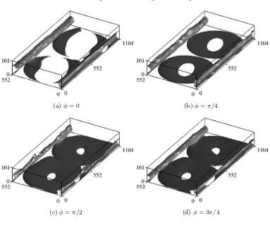
The disc flow for D+ _{= 552, W}+ _{= 13.2 and T}+ _{= 411 (R = 17%) is visualized}

at different phases in figure 8. Isosurfaces of q+ ₌ q_u+2

d +w

+2

4 4 3 3

7 8 8 7

5 7 6 6

0 3 2 3

0 200 400 600 800 1000

3 6 9 12

0.5

2.0 2.0 2.0 1.5

1.0 1 6 -9 8 W + T+

(a)D= 1.78

2 4 4 4

4 11 11 12

7 16 16 16

8 15

17 16

0 200 400 600 800 1000

3 6 9 12 5.5 2.5 6.0 3.0 5.0 2.5

1.0 2.0 2.0

12 18 20 8 W + T+

(b)D= 3.38

2 3 4 4

6 10 11 11

10 15 17 18

11 15

19 20

0 200 400 600 800 1000

3 6 9 12 5.5 0.5 6.0 4.5 2.5 1.6 5.0 2.5 1.5 5.5 3.0 19 8 19 23 W + T+

(c)D= 5.07

2 2 2 2 3 3 3

5 7 7 8 9 9 10

9 10 11 12 14 15 16

13 13 17 19

0 200 400 600 800 1000

3 6 9 12 4.0 1.0 5.5 2.5 2.0 3.0 5.5 7 17 22 22 1.0 1.0 2.5 0.5 4.5 3.5 2.0 W + T+

(d)D= 6.76

Figure 7: Plots of R(T+_{, W}+_{)(%). Scaling is performed usingu}∗

τ from the native case. The dark grey circles indicate RH13’s data and the boxed values denote positive Pnet values.

between discs, which extend vertically up to almost one quarter of the channel height. They occur where there is high tangential shear, i.e. where the disc tips are next to each other and rotate in opposite directions, but also over sections of stationary wall. They persist almost undisturbed across the entire period of oscillation, their intensity and shape being only weakly modulated in time. The thin circular patterns on top of the discs instead show a strong modulation in time. This is expected as the patterns are directly related to the disc wall motion. Although atφ= 0 the disc velocity is null, the circular patterns are still observed as the rotational motion has diffused upward from the wall by viscous effects. Instantaneous isosurfaces of low-speed streaks in the proximity of the wall (not shown) reveal that the intensity of these structures is weakened significantly, similarly to the steady disc-flow case.

Contour plots of ud in x−z planes are shown in figure 9. The first column on the left shows the contour at the wall. At y+ _{= 4 and y}+ _{= 8, the disc outlines can still}

(a)φ= 0 (b)φ=π/4

(c)φ=π/2 (d)φ= 3π/4

Figure 8: Disc-flow visualisations of q+_{(x, y, z) =} q_u+2

d +w

+2

d = 2.1 at phases φ = 0, π/4, π/2,3π/4. The disc tip velocity at each phase is shown in figure 5 (right). In this figure and in figures 9, 10, 11, and 13,D+_{= 552,W}+_{= 13.2,T}+_{= 411.}

patters created by the disc motion are displaced in the streamwise direction by the mean flow. The magnitude of the shift increases with distance from the wall and aty+_{= 8 it}

is about 100ν∗_/u∗

τ. Aty+= 27 the disc outlines are no longer visible and the structures occurring between discs in figure 8 here appear as streamwise-parallel bands ofud which do not modulate in time and are slower than the mean flow. They also appear at higher wall-normal locations up to the channel half-plane, with their width increasing with height.

The contour plots in figure 10 show the ensemble- and time-averaged wall-shear stress. At phasesφ= 0 andπ, when the angular velocity of the discs is zero, the wall-shear stress is almost uniform over the disc surface. During the other phases of the cycle, the lines of constant stress are inclined with respect to the streamwise direction and the maximum values are found near the disc tip. The lines show a maximum inclination of about 45◦

at phasesφ= 3π/4,7π/4, when the deceleration of the discs is maximum.

x+

(a)φ= 0

z

+

(b)φ=π/4

(c)φ=π/2

(d)φ= 3π/4

-12 -8 -4 0 4 8 12

0 552 1104 0 552 1104

0 552 1104 0 552 1104

0 552 0 552 0 552 0 552

Figure 9: Contour plot ofu+d(x, y, z) as a function of phase in thex−zplane aty+= 0, y+= 4,y+= 8 andy+= 27 (from left to right).

(a)φ= 0

z

+

(b)φ=π/4

(c)φ=π/2

x+

z

+

(d)φ= 3π/4

x+

-0.015 -0.01 -0.005 0 0.005 0.01 0.015 0.02 0.025

0 552 1104

0 552 1104

0 552 0 552

Figure 10: Contour plot of phase-averaged streamwise wall friction, 2h∂u+_/∂y+_| 0i/U

+2

b . The skin-friction coefficient isCf = 6.79·10−3.

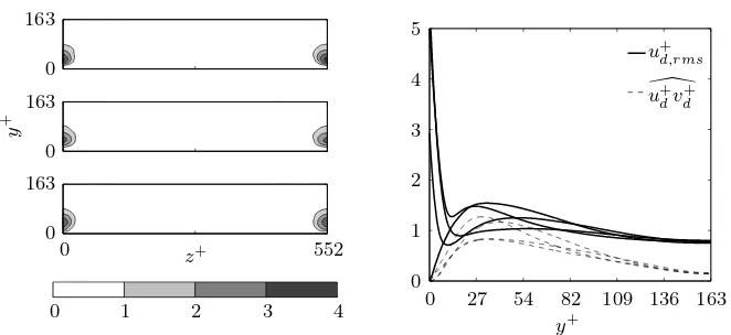
hudvdi because, although ud is significant, vd is negligible. Only the contribution to hudvdi from both negative ud and vd is included in figure 11 (left) as ud and vd with other combinations of signs only negligibly add to the total stress. The structures are therefore jets oriented toward the wall and backward with respect to the mean flow.

y

+

z+

0 1 2 3 4

0 552

0 163 0 163 0 163

y+

u+

d,rms

\

u+

dv

+

d

0 27 54 82 109 136 163 0

1 2 3 4 5

Figure 11: Left: Isosurfaces ofhu+dvd+iobserved from they−zplane atx+= 0,x+= 160, x+ _{= 320 (from left to right). The plot shows only hu}+

dv

+

difor ud, vd <0 as within the contour range the contributions from other combinations of ud and vd are negligible. Right: Wall-normal profiles of theu+_d,rms (solid lines) andu\+_dv_d+ (dashed lines). Profiles are shown for phases from the first half of the disc oscillation.

disc streamwise velocity component, defined asud,rms(y, τ) =

q c

u2

d, and of the Reynolds

stresses \u+_dv_d+ (where here the spatial average_b·does not include the time average as in (2.6)). Four profiles are shown for each quantity, for phases from the first half period of the oscillation. Data from the second half are not shown as the profiles coincide at opposite oscillation phases. The disc flow penetrates into the channel up to y+ _{≈ 15.}

When the disc tip velocity is close to its maximum, the profiles of ud,rms and wd,rms (the latter not shown) decay from their wall value and follow each other closely up to

y+ _{≈ 10. At higher locations, the magnitude ofu}+

d,rms is larger than that of the wall-normal and spanwise velocity profiles. In the bulk of the channel, fory+_{>50, the profiles}

modulate only slightly in time. This therefore further confirms that the intense temporal modulation of the disc flow is confined in the viscous sublayer and buffer region.u+_d,rms

decays to ≈ 0.7 as the channel centreline is approached. As expected, the Reynolds stresses \u+_dv_d+ show a slow time modulation and are always positive, proving that the streamwise-elongated structures favourably contribute to the drag reduction throughRd in (4.3). Neitheru+_d,rms nor\u_d+v_d+ modulate in time fory+_>120.

4.5. Power spent

4.5.1. Comparison with laminar power spent

0 10 20 30 40 50 0

10 20 30 40

Ps

p

,t

(%

)

Psp,l(%)

Pnet>0 Pnet<0

0 10 20 30 40 50

0 10 20 30 40

Ps

p

,t

(%

)

Psp,l(%)

T = 13 T = 33 T = 65 T = 130

Figure 12: Left: Psp,t(%), computed through DNS via (2.12), vs. Psp,l(%), computed through (3.6), the power spent by an infinite disc oscillating beneath a still fluid. Data are coloured according toPnet. Right:Psp,t(%) vs.Psp,l(%), with symbols grouped according toT.

predicted more accurately by the laminar solution than for cases with negative Pnet, a result also found by RH13.

Figure 12 (right) presents the same data of the right plot, with the symbols coloured according toT. The agreement is best for the largest oscillation periods,T = 130, and it worsens asT decreases. The trend forT = 130 closely resembles the one of the steadily rotating discs by RH13, which is consistent with the wall forcing becoming quasi-steady at large periods. ForT = 130, the highest value of Psp,t= 37%, occurring forD= 1.78, W = 0.51, differs fromPsp,l by 17%, while a disagreement of 15% is found by RH13 for the samePsp,l value.

4.5.2. Turbulent regenerative braking effect

For the majority of oscillation cycle, power is spent by the discs to overcome the frictional resistance of the fluid. However, for part of the oscillation and over portion of the disc surface, work is performed by the fluid on the disc. This is a form of regenerative breaking effect and it also occurs in time for the case of uniform spanwise wall oscillations and in space for the steady rotating disc case (RH13). Contour plots of the localized power spentWt, defined as

Wt(x, z, τ)(%) =

100Rp

R2

τUb ud

∂ud

∂y

y=0

+wd

∂wd

∂y

y=0 !

, (4.4)

x+

x+

z

+

0 552 1104 0 552 1104

552

0

-120 -100 -80 -60 -40 -20 0 20

Figure 13: Spatial variation ofWt, computed via (4.4), forφ=π/4 (left) andφ= 3π/4 (right). The white areas over the disc surfaces for whichWt>0 denote locations where the fluid is performing work onto the disc. The areas of regenerative braking predicted by the laminar solution, i.e. whereWl>0 and (3.15) applies, are enclosed by the dashed lines.

θ ur, uy

Structures between discs:

Rd∝R01(1−y)hudvdidy

Degradingθ-effect (Zhou & Ball 2008): Radial-flow spanwise forcing Oscillating-wall mechanism,uθ

(Riccoet al._2012):

Radial-flow streamwise forcing

Rt∝R01(1−y)

d

utvt− hu\t,svt,si

dy Mean flow

1

Figure 14: Schematic of the two mechanisms responsible for drag reduction induced by oscillating discs. One mechanism is linked to the attenuation of the turbulent Reynolds stresses and is quantified byRtin (4.2). The degrading effect of the oscillation angle θ (Zhou & Ball 2008) is represented by the shading. The second mechanism is due to the structures between discs and is quantified byRd in (4.3). The radial streaming induced by the Rosenblat pump is denoted by the open arrows.

4.6. A discussion on drag reduction physics and scaling

The results in the preceding sections prove that the oscillating discs effectively modify the flow in two distinct ways, which are discussed in the following and illustrated in figure 14.

• Role of disc boundary layer

The circular pattern which forms over a disc as a direct consequence of the disc rotation (shown in figure 8) is a thin region of high-shear flow. The laminar analysis suggests that this oscillatory boundary layer resembles the oscillating-wall Stokes layer (of thickness

δ∗

s = √

ν∗_T∗_{) at high frequency (refer to §3.2.1 when γ ≪1), and the Ekman layer of}

the von K´arm´an viscous pump (of thicknessδ∗ e=

p

ν∗_D∗_/(2W∗_{)) at high periods (refer}

over the disc surface is modified similarly to the oscillating-wall case at high frequency and to the steady-rotation case studied by RH13 at high periods. The parameter γ, written as γ = (2/π) (δ∗

s/δ ∗ e)

2

, can be interpreted as the threshold that distinguishes these two limiting regimes. The thinner boundary layer between these two limits dictates the way the turbulence is altered. Whenγ=O(1), an intermediate oscillating-disc forcing regime is identified, for which viscous effects diffuse from the wall due to both unsteady oscillatory effects and to large-scale rotational motion.

Whenγ≪1, the drag-reduction mechanism is analogous to the one advanced by Ricco

et al.(2012) for the oscillating-wall flow, namely that the near-wall periodic shear acts to increase the turbulent enstrophy and to attenuate the Reynolds stresses. Important differences from the oscillating-wall case are i) the wallward motion of high-speed fluid, entrained by the disc oscillation from the interior of the channel, ii) the radial-flow effects due to centrifugal forces, which are proportional to the nonlinear termF′2 _{(refer to (3.2)}

for the laminar case) and produce additional spanwise forcing in planes perpendicular to the streamwise direction, iii) the radial dependence of the forcing amplitude, and iv) the degrading effect on drag reduction due to wall oscillations which are not spanwise oriented. The latter effect was first documented by Zhou & Ball (2008), who proved that spanwise wall oscillations produce the largest drag reduction, while streamwise wall oscillations lead to approximately a third of the spanwise-oscillation value. The shading on the disc surface in figure 14 illustrates the effectiveness of the wall oscillations at different orientation angles.

• Role of quasi-steady inter-disc structures

The second contribution is from the tubular interdisc structures, which are streamwise-elongated and quasi-steady as they persist throughout the disc oscillation. They are primarily synthetic jets, an indirect byproduct of the disc rotation (as in RH13) or disc oscillation. As discussed in §4.4, these jets are directed wallward and backward with respect to the mean flowum. The time-averaged flow between discs is therefore retarded with respect to the mean flow. Further insight into the generation of these structures could lead to other actuation methods leading to a similar drag reduction benefit. Although the structures appear directly above the regions of high shear created by neighbouring discs in the spanwise direction, they are largely unaffected by the time-modulation of the shear. These structures could be a product of the interaction between the radial streaming flows of neighbouring discs, which have a non-zero mean (refer to figure 4 (left)).

The FIK identity is useful because the role of disc boundary layer on drag reduction is distilled into Rt, which sums up the decrease of turbulent Reynolds stresses, while the role of the structures is given byRd, which is solely due to the additional disc-flow Reynolds stresses.RtandRd quantify mathematically the two drag-reduction effects.

It has been shown that drag reduction scales linearly with the penetration depth of the laminar layer for different spanwise wall forcing conditions, such as spatially uniform spanwise oscillation, travelling and steady wall waves (Riccoet al.2012; Cimarelliet al.

laminar flow solution best represents the disc boundary layer flow because of the limited interference between discs.

From the envelope of the Stokes layer velocity profile engendered by an oscillating wall

We+=Wm+exp

−pπ/T+_y+_,

Choiet al.(2002) defined the penetration depth as

yd+=

p

T+_{/πln W}+

m/Wth+

,

whereW+

m is the maximum wall velocity and Wth+ is a threshold value below which the induced spanwise oscillations have little effect on the channel flow. For the oscillating disc case, the enveloping function for the laminar azimuthal disc velocity,W+

e =W+Ge(η, γ), where

Ge(η, γ) = max

˘

t G(η, ˘

t, γ),

plays a role analogous to the exponential envelope for the classical Stokes layer. Defining the inverse ofGe,L=G−e1, the penetration depth of the oscillating-disc layer is obtained as

δ+=pT+_{/πL W}+_/W+

th

. (4.5)

Note that in the limit ofγ→0 one finds lim

γ→0L W

+_/W+

th

= ln W+/W_th+.

The Stokes layer penetration depth is therefore obtained as a special case. In figure 15 (left), the drag-reduction contributor Rt shows a satisfactory linear scaling with the penetration depth, computed via (4.5) withW_th+= 2.25.

In order to find a scaling forRd, the portion of drag reduction only due to the inter-disc structures, the FIK identity and the laminar solution inter-discussed in §3 are employed. From (4.3), it is evident that Rd is proportional to uddvd. Through the definitions of the laminar velocity components (3.1),ud∼W andvd ∼W

√

T. It then follows that a reasonable estimate could beudvd∼W2

√

T at the edge of the discs where the structures appear. It is then logical to look for a scaling of Rd in the formWmTn. An excellent linear fit for the drag reduction data is found for (m, n) = (2,0.3), as shown in figure 15 (right). Outer-unit scaling forW andT applies, which means that the structures are not influenced by the change inu∗

τ. The exponent of W is as predicted by the laminar solution. The deviation of the coefficientn from that predicted by the laminar analysis (i.e. n= 0.5) can be accounted for by the factors which are not taken into account in the laminar analysis, such as the disc-flow interaction with the streamwise turbulent flow and between neighbouring discs.

5. Outlook for the future

0 2 4 6 8 10 12 2

4 6 8 10 12

Rt

(%

)

δ+

0 0.1 0.2 0.3 0.4 0.5 0.6 0

1 2 3 4

Rd

(%

)

W2

T0.3

Figure 15: Left:Rt, the contribution to drag reduction due to turbulent Reynolds stress attenuation, vs.δ+_{, the penetration depth, defined in (4.5). Right:R}

d, the contribution to drag reduction due to the disc-flow Reynolds stresses, vs. W2_T0.3_{. The diameter is}

D= 6.76. White circles: W+_{= 3, light grey:W}+_{= 6, black:W}+_{= 9.}

the oscillation frequency in the present case (f∗

= 2π/T∗

) and the rotational frequency in RH13’s case (f∗

=ω∗

/2π, where ω∗

is the angular velocity).

Experimental realisation of the disc-flow technique is possible with D∗

= 4−8 cm,

W∗

= 0.2 m/s in a water channel and 4.6 m/s in a wind tunnel. The frequencies aref∗

= 0.37 Hz and 16 Hz, respectively. The dimensional parameters in flight areD∗

= 5.8 mm,

W∗

= 70.7 m/s, and f∗

= 1752 Hz. Commercially available electromagnetic motors (D∗

= 2 mm, f∗

=O(103) Hz), adapted for oscillatory motion, would guarantee these time and length scales of forcing (Kuang-Chen Liuet al.2010). The optimal frequency in flight is approximately half of the optimal one for steady rotation:f∗ _{= 1752 Hz for}

the oscillating discs compared tof∗_{= 3718 Hz for the steady rotating discs.}

Figure 16 shows characteristic time and length scales of the oscillating-disc technique and of other drag reduction methods. The typical length scale of the oscillating-disc technique is larger than that of the steadily rotating discs and the standing wave forcing, whilst being two orders of magnitude greater than both riblets and the feedback control systems studied by Yoshinoet al. (2008). The typical time scale of the oscillating disc flow is one order of magnitude larger than that of the oscillating wall forcing. It is also worth pointing out that these are optimal values for the tested parameter range and that our results in §4.2 hint at the possibility to obtain comparable drag-reduction values for even larger oscillation periods and diameters, which are denoted by the dashed lines in figure 16.

The notable limitation of our analysis is the low Reynolds number of the simulations. It is therefore paramount to investigate the disc-flow properties at higher Reynolds number to assess whether and how the maximum drag reduction values and the optimal forcing conditions vary.