Modeling ventricular-vascular coupling in the developing embryo

(1)

Rochester Institute of Technology

RIT Scholar Works

Theses

Thesis/Dissertation Collections

9-1-1996

Modeling ventricular-vascular coupling in the

developing embryo

Michael Bauman

Follow this and additional works at:

http://scholarworks.rit.edu/theses

This Thesis is brought to you for free and open access by the Thesis/Dissertation Collections at RIT Scholar Works. It has been accepted for inclusion

in Theses by an authorized administrator of RIT Scholar Works. For more information, please contact

ritscholarworks@rit.edu

.

Recommended Citation

(2)

MODELING VENTRICULAR·VASCULAR

COUPLING IN THE DEVELOPING EMBRYO

by

Michael G. Bauman

A Thesis Submitted

III

Partial Fulfillment

of the

MASTER OF SCIENCE

III

Mechanical Engineering

Approved by:

Mark H. Kempski, Ph.D.

Department of Mechanical Engineering

Kevin B. Kochersberger, Ph.D.

Michael P. Hennessey, Ph.D.

Charles W. Haines, Ph.D.

(Thesis Advisor)

(Department Head)

College of Engineering

Rochester Institute of Technology

Rochester, NY 14623

(3)

Release

I, Michael G. Bauman, do hereby give permission to Wallace

Memorial Library to reproduce this Thesis, entitled Modeling

Ventricular-Vascular Coupling in the Developing Embryo, in whole or in part. Any

such reproductions may not be for commercial use or profit.

Signed,

Michael G. Bauman

9-

23-90

(4)

Table

of

Contents

List

of

Tables

List

of

Figures

Abstract

iv

Vll

1.

Introduction

1

1.1

Congenital Cardiovascular Malformations

1

1.2

Research Objectives

2

1.3 Thesis

Objectives

and

Goals

3

2.

Methodology

6

2.1

Modeling

6

2.1.1

Modeling

Hemodynamic Systems

6

2.1.2 Model Rationale

7

2.1.3 Model Simulation

11

2.1.4

Simulink

16

2.1.5 State Space

and

Block

Diagram Formulation

1

8

2.1.6 Initial Conditions

24

2.2

Optimization

Techniques

26

2.2.1 Design Variables

26

2.2.2 The Method

of

Least Squares

27

2.2.3

Numerical

Optimization

Techniques

29

(5)

2.3

Preparation

of

Data

35

2.3.1 Data Acquisition

35

2.3.2 Data

Filtering

and

Conversion

35

2.3.3 Assumptions

36

3. Results

41

3

.

1 Verification

of

Simulation

and

Optimization

Routines

4 1

3.1.1

Benchtop

Circuit

Setup

41

3.1.2 Model 1 Test Results

42

3,1.3 Model 2 Test

Results

43

3.1.4 Model 3 Test

Results

44

3.1.5

Comments

45

3.2

Results

of

Blood Data

Simulation

and

Optimization

46

3.2.1

Convergence

Criteria

46

3.2.2

Model

1

Results

47

3.2.3 Model 2

Results

51

3.2.4 Model 3

Results

56

3.2.5

Multiple

Cycle

Simulation

Results

60

4.

Discussion

and

Conclusions

6.2

4.

1

Validity

of

Simulations

62

4.2

Recommendations

for

Future

Studies

65

(6)

Appendices

68

Appendix

A

Algorithm Flow

Chart

68

Appendix B

MATLAB

m-files

69

B.l

INTERP.m

70

B.2

OBJILSC.m

71

B.3

OBJlLSL.ni

73

B.4

OBJILSC.m

75

B.5

OBJ2LSL.m

11

B.6

OBJ3LSC.m

79

B.7

OBJ3LSL.m

81

(7)

List

of

Tables

Table

Description

Page

Section 3

3-1

Model 1 Test Results

42

3-2

43

3-3

44

3-4

Model

1

Constant

Parameter Optimization

Results

49

3-5

Model 1

Linearly Varying

Parameter Optimization Results

50

3-6

Model 2 Constant Parameter Optimization Results

54

3-7

Model 2

Linearly Varying

55

3-8

Model 3 Constant Parameter Optimization Results

58

3-9

Model 3

Linearly Varying

59

(8)

List

of

Figures

Figure

Description

pase

Section

1

1-1

Formation

of

the

Heart

2

1-2

Schematic

of

Heart

and

Adjoining

Vasculature

4

Section

2

2-

1

Lumped Parameter Fluid I-C-R

Model

6

2-2

Windkessel Afterload

Model

8

2-3

Model 1:

Resistive-Capacitive

Model

of

Aortic Arches

9

and

Conotruncus

2-4

Model 2: Series Inertance Model

of

Aortic Arches

and

9

Conotruncus

2-5

Model 3: Parallel Inertance Model

of

Aortic Arches

10

and

Conotruncus

2-6

Basic R-C-R Circuit

1 1

2-7

Plot

of

Output Voltage for R-C-R Circuit Test Case

1

3

2-8

Plot

of

MATLAB Simulation Output for R-C-R Circuit

1 5

2-9

Block Diagram Representation

of a

System Transfer

16

Function

2-10

Model 1: Resistive-Capacitive Model

of

Aortic Arches

18

and

Conotruncus

2-11

Model 1 Block Diagram

19

2-12

Model 2: Series Inertance Model

of

Aortic Arches

and

20

Conotruncus

2-

1

3

Model 2 Block Diagram

2 1

(9)

Figure

Description

Page

2-15

Model 3 B lock

Diagram

23

2-16

Model 1: Electrical

Benchtop

Test Case Circuit

30

2-17

Plot

of

Benchtop

Test Results

Using

LEASTSQ.m

33

2-18

Unfiltered Pressure

and

Volume Data

35

2-19

Filtered Pressure

and

Flow Data

36

2-20

Multiple Pressure

vs.

Volume Traces (P-V

Loops)

38

2-2 1

Ventricular-Vascular

Coupling

Window

of

Opportunity

39

Section 3

3-1

Model 1

Benchtop

Optimization Results

42

3-2

Model 2

Benchtop

Optimization

Results

43

3-3

Model 3

Benchtop

Optimization

Results

44

3-4

Model 1 Constant Parameter Best Fit

48

3-5

Model

1 Linear

Parameter

Best Fit

48

3-6

Model

2 Constant

Parameter

Best

Fit

52

3-7

Model 2 Linear Parameter Best Fit

52

3-8

Model

2 Constant

Parameter

Worst

Fit

53

3-9

Model

2 Linear

Parameter

Worst Fit

53

3-10

Model

3 Constant

Parameter

Best Fit

57

3-

1 1

Model

3

Linear Parameter

Best Fit

57

(10)

Abstract

Congenital

cardiovascular

malformations

are

one

of

the

major

contributors

to

infant mortality

in

the

United

States

today.

Defects

in

the

cardiovascular

system

are

evident

at

very early

stages

in

the

developing

embryo,

yet

there

exists

no

substantial

diagnostic

tool(s)

for

recognizing

defects

at

these

early

stages.

Cardiac

morphogensis occurs

throughout the

pre-innervated period

of

embryonic

development.

It

is

speculated

that the

flow

of

blood

during

the

early

embryonic stages plays an

important

role

in

the

development

of

the

cardiovascular

system.

Blood

flow

is

a

possible

mechanism

for

communication

between

the

heart

and

vasculature,

contributing

to

cardiac

development.

The

objective

of

this

study is

to

investigate

ventricular-vascular

coupling

across

the

conotruncus

and

aortic

arches

using

mathematical

models

to

simulate

experimental

hemodynamic data from

a

Stage

21

White Leghorn

chick

embryo.

Lumped-parameter

hydraulic

models of

the

embryonic

vasculature

are

tested

for

their

ability

to

predict

experimental

data

using Least Squares

minimization

techniques.

This

(11)

Chapter 1

-

Introduction

1.1

Congenital

Cardiovascular

Malformations

Congenital

cardiovascular

malformations

are

one

of

the

major contributors

to

infant

mortality

in

the

United

States

today

(Clark

and

Takao 1990).

Cardiovascular

malformations

may

also present

themselves

as a major

health

risk

later in life.

Detecting

birth

defects,

and

in

particular

those

cardiovascular

system,

early in fetal development has been

a

goal of

many

researchers.

Thus far

there

have been very few

tools to

act as

indicators

of

cardiac malformations

during

embryonic morphogenesis.

The heart is

the

first

functioning

organ

in

the embryo,

beginning

to

beat

well

before

the

existence

of a nervous system.

In

the

human,

the

heart begins

to

beat 22 days

after

conception.

At only

a

day

after

the

heart

starts

beating,

it

begins

to

fold

and

develop

into four

distinct

chambers

known

as

the

right and

left

atrium and

right and

left

ventricle.

From

a

primitive muscle-wrapped

tube,

the

heart

undergoes

a

very

complex and continuous period of

development (see Figure

1-1),

and

if

all

goes

right,

ending

with

a

four-chambered blood

pump,

complete with

valves

and neural control system.

During

the

morphogenesis of

the

heart,

there

exist

numerous

(and

quite

possibly

infinite)

occasions

for

malformations

to take

place,

thus

making it

remarkable

that

a

majority

of

hearts

turn

out

"correct."

This

raises

the

important

question,

"Why

do

most

hearts (and

infants)

turn

out

fine,

while others

do

not?"

What

are

the

factors

that

contribute

to the

development

of

the

heart,

and

what

is

the

controlling

mechanism

in

cardiovascular

morphogenesis when

there

is

an absence of

a

central

(12)

[image:12.562.203.371.59.171.2]

Figure 1-1.

Formation

of

the

heartfrom

a muscle

wrapped

tube.

While

cardiovascular malformations are not

limited

to

any

one

specific

area,

it

has

been

shown

that

ventricular

septal

defects

are

perhaps

the

most

common

of

all

heart

malformations

occurring in live-born infants (Human

Embryology

1993).

Along

with

this

are malformations such as

double

outlet

left

ventricle and

transposition

of

the

great

vessels.

Some

malformations

may

not

be detected

throughout

embryonic

development,

and

only

become painfully

apparent when a person

has become

an

adult.

Anomalies

with

the

mitral

valves are quite common

in

adults,

yet are

rarely life

threatening

(Human

Embryology

1993).

Early

detection

of such malformations often allows

treatment

and

in

some cases

the

saving

of

a

life,

thus

a good

understanding

of

the

processes

and

functions involved

with morphogenesis

become

a great

concern.

1.2

Research

Objectives

The

long

term

and

overall scope of

the

research

presented

in

this

thesis, along

with

paralleled

research,

is

to

foster

the

prevention of

life

threatening

birth defects

through the

sciences of

engineering

and medicine.

The

short

term

objectives associated with

this

research

are aimed at

understanding

the

hemodynamics

occurring in

the

pre-innervated

embryo,

and

to

find

methods of

recognizing

(13)

The

focus

is

to

utilize

engineering

tools

as

a

means

of

describing

hemodynamic function

within

the

normally developed

embryonic

cardiovascular

system.

1.3

Thesis

Objectives

and

Goals

The

primary focus

of

this thesis

is

to

investigate

the

existence of

coupling

in

stage

21

White

Leghorn

chicken embryos

through

various

hydraulic modeling

scenarios.

Stage 21

represents

about

3.5

days

into

the

gestation

period

for

the

chicken

embryo,

which

translates

to

about

45

days

into

the

human

gestation

period,

according

to the

Hamburger-Hamilton

(Hamburger

and

Hamilton

1951)

scale

of embryonic

development.

At

this

stage,

as mentioned

before,

there

exists no autonomic

nervous system

to

control cardiac

function.

The

material presented

in

this thesis

is

an extension of previous

work as

well

as

an

exploratory

effort

in hemodynamic

modeling.

It is

speculated

that the

flow

of

blood

during

the

early

embryonic

stages

plays

an

important

role

in

the

development

of

the

heart

and vasculature

(Hu

and

Clark 1989). In

some

cases,

deliberate shunting

of

blood

flow

or

slight

changes

in

the tissue

composition

(i.e.

treatment

with retin

A)

has induced drastic

changes

and malformations

in

cardiovascular

development (Broekhuizen 1995). This

research

has

pointed

in

the

direction

of

blood flow

as

being

a medium

for

physiologic

communication

during

morphogenesis.

In

the

pre-innervated

embryo,

there

exists

no

autonomic nervous

system

to

control

blood

flow,

yet

there

exists

strong

evidence

to

support

the

theory

of

hemodynamic

regulation on a

beat

to

beat basis

(Kempski

et

al

1993).

Hemodynamic

pressure

has been

hypothesized

to

respond

to

a

resistance

to

flow

associated

with

vascular

impedance,

indicating

possible

hemodynamic

(14)

During

early

stages

of

development,

the

vasculature

just

proximal

the

left

ventricle

undergoes several

changes.

The

outflow

tract

from

the

left

ventricle

begins

as

a

bulb-like

formation

known

as

the conotruncus

(bulbus

cordis),

and

eventually

septates

and transforms

into

the

mature semilunar valve.

During

early

cardiovascular

development

several vascular

branches known

as

the

aortic arches sprout

from

the

early

outflow

tract, known

as

the

aortic

arches which

transform

during

subsequent

development

stages

into

what will

later become

the

major

arteries

in

the

adult.

Further

downstream

is

a

multitude

of

vessels

that

will

eventually

extend

throughout

the

adult

body.

Conotruncus

Aortic Arches

flightand lett-anterior cardinal veins

Ventricle

Rightandleftumbilical arteries

Figure 1-2. Schematic

representation

of human heart

and vasculature at

approximately 25

days

after

conception.

Studies have

shown

that

coupling may

exist

early

on

in

cardiac

development,

and

may

act as

a

regulatory

mechanism

for

cardiac

development.

Even in its

earliest

form,

the

conotruncus acts

to

regulate

blood flow

out of

the

heart,

and

keep

blood

from regurgitating back into

the

ventricle.

The

conotruncus

may play

a

vital

role

in

(15)

1989).

The function

and

health

of

the

conotruncus,

therefore,

may

act as a

mechanism and/or

indicator for

the

development

of

malformations

associated

with

the

left

ventricle and

the

adjoining

vasculature.

Developing

a

mathematical model

to

represent

the

physiology

within

a

section of

the

vasculature which

includes

the

ventricle,

conotruncus,

aortic

arches,

and

distal

vasculature

then

becomes

the task

at

hand (Matalevich

1995,

Mates

et

al

1982,

Kempski

et al

1993,

1995).

has

demonstrated

the

use of electrical circuit-type models

in

simulating

the

dynamics

of

blood flow

through

various parts

of

human

and

non-human vasculature.

Lumped

parameter models

involving

resistors,

capacitors,

and

inductors have been

used

to

simulate

the

resistive, elastic,

and

inertial

characteristics,

respectively,

associated with

the

blood

and/or

blood

vessels.

Varied degrees

of

success

have

been

achieved

in using linear

forms

of

these

models,

such

as

the

classic

Windkessel

model,

to

represent

vascular

impedance

and

coupling

associated with

blood flow

and pressure

(Kempski

1994,

Matalevich

1996).

This study

will

investigate

the

application of

these

linear lumped

parameter circuit

models

to

simulate

physiologic

occurrences

across

the

conotruncus

and

aortic

arches.

Various

models

will

be

postulated

and

tested

for

goodness

of

fit,

parameter

sensitivity,

linearity,

and

physiological relevance.

This study

will

also

evaluate

the

use of commercial

PC

-based software

as a

tool

for

cardiovascular research.

The

work

presented

in

this

paper

will

be

used as a

benchmark for future

studies

in

the

area

of

coupling

and

(16)

Chapter 2

-Methodology

2.1

Modeling

2.1.1

Modeling

Hemodynamic

Systems

Blood flow

through the

human

vasculature

is

a

hydraulic

or

fluid

system

in its

simplest sense.

Blood flow is dependent

upon pressure variations

throughout the vasculature,

which

in

turn

is

a

function

of vascular resistance

to

flow,

distensibility

of

the

vessel

walls,

and

inertial

effects associated with

the

blood itself.

Though

numerous

factors

contribute

to

the

blood flow

characteristics

in any

part

of

the vasculature,

simple

"lumped"

parameter

models of a

fluid

system can

be

used

to

represent a

sum

total

of

these

factors for

the

ease of

simulating

the

dynamic

performance

within a particular

area of

the

vasculature.

Figure 2-1

shows a

typical

lumped

parameter model

of a

fluid

system.

f

~

c

=

'

K

_s

/

////7//S7

Pa

X

\

'Piston and

Spring

(Ap

=_piston

area)

Rf

sFluid

"Slug"

(Acs

=_cross_{sectional area of}

slug)

'/

=

pL

cs /

figure 2-1. Lumped

parameter

fluid I-C-R

model.

Volumetric flow from

the

heart,

Qh

is

the

(17)

Model

Parameters

for

a

Hydraulic

(Fluid)

System:

q

:

volume

[ml]

Q

:

volumetric

flow

rate

[ml /

sec]

P

:

pressure

[mmHg]

R

:

resistance

[mmHg

sec

/ml]

C

:

capacitance

[ml

/mmHg]

I

:

inertance

[kg

/mm4]

As

with

any

dynamic

system,

there

exists a set of

governing

equations which

describe

how

the

system

behaves.

For

a

hydraulic

system, the

elemental equations

relating fluid flow

and pressure

(differential)

to

the

system parameters are as

follows:

Pbc=*/Q3

(2-1)

Pab=//iir

(2,2)

dP

Q2

=

C,

-f-(2.3)

dt

And

by

the

laws

of

continuity,

we can

write

an expression

relating

the

flow

through

various parts

of

the

system

as:

Qi

=

Q2

+

Q3

(24)

When

the

elemental equations

are

used

in

the

continuity

equation,

a

differential

equation results

which

describes

the

dynamics

of

the

system.

Pb+^Pb+^Pb=^Pa+^Pc

(2-5)

CjRj

Cj Ij

Cj Rj

2.1.2

Model Rationale

Lumped

parameter

models,

typically

in

the

form

of electrical circuit analogs

to the

hydraulic

circuits,

have been

used

with

success

in modeling

the

hemodynamics

through

both

(18)

been

used

to

simulate

the

blood

flow

through

various

vasculature

beds (Mates

1982,

Burkoff

[image:18.562.63.506.108.287.2]

1988,

Kempski

1994),

and

has

proved

to

be

a valid model

in

multiple studies

(Figure 2-2).

Figure 2-2.

Three-element Windkessel

model shown as an electrical circuit

analog

with

current source

representing

a

flow driver.

At

particular stages of embryonic

development

and

sections

of

the

vasculature

bed,

the

Windkessel

model

fits

quite

well,

while

it

seems

to

lack

performance

in

other areas

of

study.

At

stage

21

of

the

Leghorn

chick

embryonic

development,

the

vasculature

bed

includes early forms

of

the

conotruncus and aortic arches.

At

this

stage

the

conotruncus

is

not much

more

than

a

bulbus

muscle

formation

rather

than

a

full

fledged

valve.

The

aortic

arches are

arterial

branches

that

eventually

combine

during

morphogenesis

to

form

a single

aorta.

While

the

Windkessel

model

may accurately

predict

dynamics

downstream

of

the

arches,

also referred

to

as

"afterload",

it is

speculated

that

additional

parameters need

to

be

introduced

to

represent

the

dynamic

characteristics associated

with

the

additional

physiologic

features.

Assuming

a compliance

is

associated

with

both

the

aortic

arches

and

conotruncus,

along

with

an

impedance due

to the

addition

of

the

aortic

arches,

we

can postulate a

(19)

^Taa

Rvi

AA/V

[image:19.562.59.505.440.619.2]

c

Figure 2-3.

Model 1:

resistive-capacitive

model

of

aortic arches and conotruncus with

Windkessel

model

representing

afterload presented

by

the

distal

vasculature.

Rvl, Rv2,

and

Cv

represent

the

parameters associated

with

the

downstream

vasculature

(afterload).

Though

the

vessels are

very

small

during

this

stage

in

embryonic

development,

the

movement of

the

blood may impose

a

relatively

significant

momentum

associated

with

a

"slug"

of

fluid

(blood)

within

the

flow.

A

slight modification

to

Model 1 in Figure

2-3

to

include

an

inertance

term,

lb,

would

allow

for any inertial

effects

having

to

do

with

the

mass

of

the

blood.

Figure 2-4

shows

the

schematic

definition

of

Model

2

with

this

inertial

system

parameter.

Figure 2-4.

Model 2:

series

inertance

model

of

aortic arches

and

conotruncus

with

(20)

If

inertance

associated

with

the

mass of

the

blood

is

a

significant

factor,

then

it is

unclear as

to

whether

it

occurs

just

posterior

to the

conotruncus,

as

portrayed

in Model

2,

or

if

there

exists an

inertial

effect right out of

the

left

ventricle

itself.

If

the

latter is

the case, the

model needs

to

be

modified

further

to

simulate

this

effect and

to

also

include

a

resistance

imposed

by

the

conotruncus.

Anticipating

the

effect of such a

system,

a

configuration

of an

[image:20.562.62.502.270.478.2]

inertor

(inductor)

in

parallel with a resistor would simulate

the

dynamics

quite

accurately.

Figure 2-5

shows

this

configuration

as

Model

3,

once

again

using

the

three

element

Windkessel

model

to

represent

the

downstream

vasculature.

Figure 2-5.

Model 3:

parallel

inertance

model

of

aortic arches

and

conotruncus with

Windkessel

model

representing

afterload presented

by

the

distal

vasculature.

With

three

models

postulated,

it is inevitable

that

one

model

will

represent

the

dynamics

of

the

system

better

than the

others.

To determine

the

validity

of each

model,

actual

data

needs

to

be

passed

through

a

simulation

of each representative

system,

and

the

system

parameters

need

to

be

optimized

such

that there

is

a

good

match

between

the

(21)

from

the

left

ventricle, Qs.

The

output

is

seen

as

the

left

ventricular

pressure,

Pa,

and

is

represented

by

the

pressure at node

(a)

in

all

three

models.

Before using

the models,

each system must

be

converted

to

a usable

form,

that

is,

a

set of

differential

equations

representing

the

dynamics

of each system.

The methodology

of

doing

this

can

be

found

in

the

next section.

2.1.3

Model

Simulation

There

are

several methods

for solving for

the

output(s)

of a

dynamic

system.

A

typical

system can

be

represented with one or more

differential

equations

in

terms

of state

variables and some sort of

forcing

function.

We'll

use an example of a

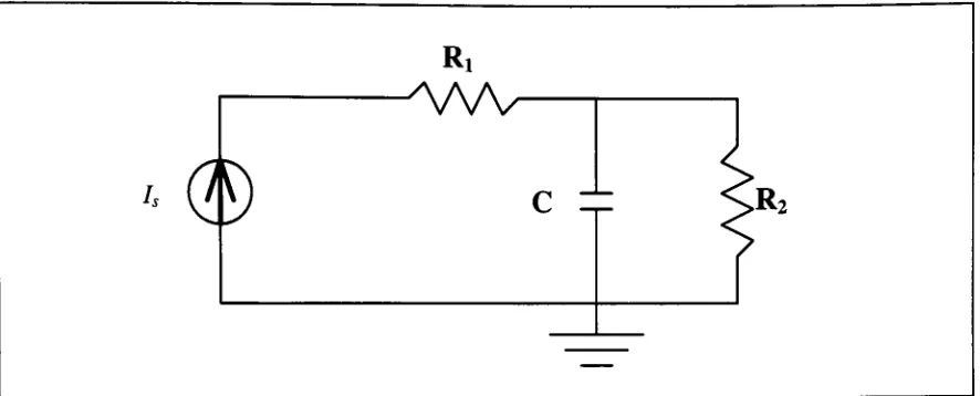
basic R-C-R

circuit

(Figure 2-6).

Figure 2-6. Basic R-C-R

electrical

circuit

Assuming

the

input

source

is

a

current

driver

as shown

in

the

diagram,

the

governing

differential

equation

for

the

system

is:

vb

+

1

(22)

Where

vb

is

the

output voltage at node

(b). The

system

time

constant

is

given

by

the

inverse

of

the

coefficient

on

the

second

term:

T

=

Ci/?2

(2.7)

It

should

be

mentioned

that

since

the

circuit

is

set

up

with

a

current

driver,

the

resistance

Ri

has

no

bearing

on

the time

constant

if

vb

is

the

desired

output.

For

a

harmonic

input,

(i.e.

Is(t)=

Is

sin(cot)),

a closed

form

solution can

be

expressed as:

Ji

+

iC^coy

From

equation

(2.8),

the

output voltage

vb

can

be

calculated

directly

from

the

input Is.

If

the

voltage

at

node

(a)

is

the

desired

output,

the

can

be slightly

modified

through the

use of

Ohm's law

to

give a closed

form

expression

for

va:

va-vb

=

iA^>vb

=

vcl-i1R1

(2.9)

va

(t)

=

7,/J,

sm(cot)

+

Is

. 2

sin(a

-<p)

(2.10)

jl

+

iC^a))2

(where

Is

is simply

the

sine amplitude

of

the

current.)

This

form

of

the

solution adapts quite well

to

least

squares optimization of circuit

parameters

using EXCEL

or other spreadsheet

solvers.

To demonstrate

this

method,

the

circuit shown

in Figure 2-6

was

built up

on

a

bread-board

and used

to

produce an output

voltage at node

(a)

when

excited

by

a sinusoidal

input

current,

Is

(The

current source

was

created

by

passing

the

output

voltage

from

a

function

generator

through

a

resistance, thus

producing

a

proportionally

scaled

current.

The

signal

was

a

zero-mean

sinusoid

of

approximately

1Hz

nominal

frequency.

Q, Ri,

and

R2

were

set

to

10u/,

17.58kQ

and

(23)

LabVIEW data

acquisition algorithm,

and

imported

directly

into

EXCEL

with

no

filtering

necessary.

The

current amplitude

Is

was

determined

from

the

data

series,

and

the

signal

frequency,

co,

was verified as

being

6.15rad/sec

(/5=0.98Hz).

With arbitrary

values given

for

Ci,

Ri,R2,

and

$,

a

sum-of-the-squares

minimization was performed

using

the

recorded

data

for

va

as a reference.

Figure

2-7

shows

the

outcome of

the

minimization with

resulting

values

for

Q, Ri,R2,

and

₀

as expected.

Though relatively

simple and

straightforward,

this

method

proves

to

be

very unaccomodating

when more complex systems are

being

investigated.

The

closed

form

solutions

to

multi-order systems with several parameters are

difficult

to

arrive

at,

so

a

state-space

formulation

of

the

governing differential

equations

is

developed,

and numerical

techniques

are used

to

solve

the

system.

Output Voltage

(Va)

for R-C-R Circuit

0.4

-0.4

Time,

seconds

-Actual

Voltage

[image:23.562.66.491.361.570.2]

Predicted Voltage

Figure 2-7. Analytic

simulation

of R-C-R

electricalcircuit.

MATLAB

employs

several

different

numerical

techniques

to

solve multi-order state

space systems

of

differential

equations.

Most

commonly,

MATLAB

makes use of

(24)

and solve

for

the

state

variables

at

discrete

time

points.

The

example

shown above could also

be

put

into

state-space

form

and solved

using

the

numerical routines

within

MATLAB.

Essentially,

we

have

a

first

order state-space

equation,

where

the

voltage

vb

is

the

state

variable,

and an output equation

for

va

using

the

same state space:

dx

dt

'

-1 "

v0

+

"

1

"

Lc>.

/,

=

[A]*(iO

-I-[fi](0

differential

equations)

y(t)

=

va=vb+

[R\ ]l,

=

[C]x(t)

+

[D]u(t)

_output

equation(s)

MATLAB

needs

only

the

A,B,C,

and

D

matrices

along

with a

vector

of

the

initial

conditions

(see Sect.

2.4,

Initial

Conditions)

on

the

states

to

produce an

output

given

an

input

u(t).

This

method makes

it very easy

to

go

from

the

state space

equations

to

a

numerical

output without

having

to

find

a closed

form

of

the

solution

for

the

system.

For

the

R-C-R

circuit

example,

we

only have

one state

variable,

vb.

An

expression can

be

written

for

the

initial

value of

vb

based

upon

the

input

Is

and

the

known

(experimental)

value of

va

at

time

t=0:

v<0) = v

-RJl0)

(2.11)

To

demonstrate

the

use

of

the

state-space

solution, the

same

system shown

in Figure

2-6

is

solved

using MATLAB. A function

called

by

LSIM,

short

for linear

simulation,

is

used

to

integrate

the

state space

equations

at

discrete

timepoints

using

an

array

of

values

for

the

input,

u(t),

which

in

this

case

would represent

the

current

in

the

R-C-R

circuit.

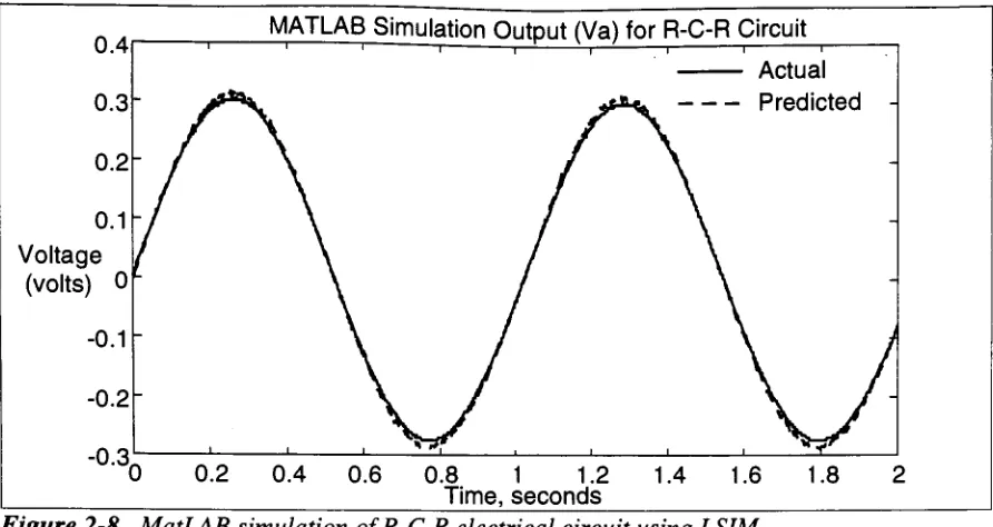
Figure 2-8

(25)

0.1

Voltage

(volts)

0L

MATLAB

Simulation

Output

(Va)

for R-C-R Circuit

Actual

[image:25.562.58.504.48.285.2]

Predicted

Figure 2-8. MatLAB

simulation

of R-C-R

electrical circuit

using

LSIM.

For

a

direct

simulation of

the system,

the

A, B, C,

and

D

matrices

are

defined

with

the

system parameters

Cl, Rl,

and

R2. For

a case where

manipulation

of

the

system

parameters

is

necessary,

such as

during

optimization,

the

matrices can

be defined in

terms

of

variables,

which are assigned values

somewhere

within

the

MATLAB

workspace.

Optimization

can

then

take

place

by

varying

the

system parameter variables

to

minimize

a particular objective

function. The

model parameters used

in predicting blood flow

need

to

be

optimized such

that

there

is

a

good

match

of

predicted

and

experimental

data.

Optimization

of

the

system

(26)

2.1.4

Block

Diagrams

and

SIMULINK

Interface

Up

until

this

point,

no

mention

has been

made

of

transfer

functions

or

block

diagrams.

Part

of

this

study includes

the

evaluation

of

desktop

software,

MATLAB

in

particular,

as a valid

tool to

be

used

in

research activities associated

with

biological

systems.

MATLAB

includes

a

package

called

SIMULINK

which

allows

simulation

of

dynamic

systems

by

defining

a

block

(simulation)

diagram

representation of

the

system

(See Figure

2-9).

s+1

Input

s2

+ s +

1

^

Output

T

ransfer

Functic

>n

Figure 2-9. Block diagram

representation

of

a system

transfer

function.

The

transfer

function

of an

entire system can

be broken up into

smaller

subsystems

that

are all

linked

together

in

the

block diagram.

Feedback

loops, integrators,

and

summing

junctions

can

all

be

extracted

from

the

system

transfer

function,

or

drawn right from

the

constitutive equations

for

the

particular system.

There

are

distinct

advantages

to

defining

a

system

in

this

manner.

First,

the

block diagram

provides a

visual

aid

in understanding

the

dynamics

and

various

pathways

associated

with

the

state

variables.

Second,

the

block

diagram

makes

it easy

to

play "what

if..."

scenarios.

That

is,

additional

blocks

and pathways

could

be

added

in

a

very

short

time

without

having

to

derive

the

analytic

expressions

defining

the

state space

of

the

model.

One disadvantage

of

using SIMULINK

over

an

analytic

formulation

of

the

state-space

is

that

computation

time

increases

as

MATLAB has

to

"convert"

(27)

beginning

of

this study, the

actual

cost

in

time

was

unclear,

but

the

results

of

this

study

should provide a good

benchmark

that

can

be

compared

to

other

forms

of

simulation.

The

SIMULINK

package works

within

the

MATLAB

workspace

just

as

any

other

m-file

or

function,

since

it is

saved as

lines

of code within

an m-file.

Within

the

m-file

is

information pertaining

to the

state

variables

of

the

system,

and

in fact

the

state space

representation of

the

system can

actually be

extracted

from

the

m-file

in

terms

of

the

A, B, C,

and

D

matrices mentioned

in Section 2.1.3.

Because

of

this,

the

same

type

of

Runge-Kutta

(28)

2.1.5

State Space

and

Block

Diagram

Formulation

of

Models

1,2,

& 3

SIMULINK

was used

in

the

solution and optimization of

the

models postulated

for

predicting

blood flow

during

this

study.

SIMULINK

can

be

called

by

any

function,

such as

LEASTSQ

(least

squares

optimization

routine,

see

Section

2.2),

making

custom sub-routines

very

simple.

But

before

a

SIMULINK

representation

of

the

model can

be

written,

the

model

must

first

be

converted

to

block diagram form

from

the

constitutive

equations

defining

the

interaction

of

the

model parameters.

The

formulation

and conversion of each

model

is

as

follows.

Model

1

figure 2-10.

Model

1:

resistive-capacitive model

of

Windkessel

afterload model.

By

continuity

we can write

the

constitutive equations:

Qs=Qi

Qi

=

Q2

+

Q3

=

Q4

+

Q5

(29)

From

the

elemental equations we can

write:

dP

1

Q2

=

cct-^Pa=3-jQ2dt

P

-P

R

_Taa

dP,

=

7^-jQ4dt

Q4

=

Caa

~ =>

?b

aa

^

b

c

ilil

P

-P

Rv,

dP

1

Q7

=

R

(2.12)

(2.13)

(2.14)

(2.15)

(2.16)

(2.17)

v2

A

block

diagram

can

be formulated

directly

from

the

constitutive and elemental

equations:

ITime.Qs]

From

Workspace

Ql

=HD- Q2

17s

3L

Pa-Pb

-n*

fg]

^i/cj>

* l/s

SL

l/Rvl Pb-Pc {35=

1/Rv2

Q6

i=HD-

07 1/Cv * l/s Pa

Pb

Pc

[image:29.562.75.482.357.593.2]

Outport

(30)

Using

the

elemental

equations

(2.12-2.17)

in

the

continuity

equations

we arrive at

the

following

state

equations:

a

PR

a

+

r

R

"b

+

p.

Qs

^ctKTaa

*~ctKTaa

^ct

(2.18)

Pb

=

^aa^Taa

P.

-+

.^aa^-Taa

^aa^vl

Pb

+

CaaRvl

(2.19)

P.

='

RVIcv

P.-

l

+

l

R.

_vl

R

ivv2

(2.20)

[image:30.562.57.508.116.487.2]

Model

2

Figure 2-12.

Model

2:

series

inertance

model

of

Windkessel

afterload model.

By

continuity

we can write

the

constitutive

equations:

Qs

=

Qi

=

Q2

+

Q3

(31)

From

the

elemental equations

we can write:

dP

1

q.-C-^p.-JLj

Q;dt

b -"-b

P.-R

dt

Q3=f

J(Pa-Pb)dt

Q3=^^

R

_Taa

dP

1

dt

P

-P

R

vl

HP

1

Q6=Cvl^=>Pd=^/Q6dt

*-(2.21)

(2.22)

(2.23)

(2.24)

(2.25)

(2.26)

(2.27)

v2

[image:31.562.72.497.75.628.2]

02 Pa .m

[Time.Qs]

21

^

1/Cct^

l/s

-Hi_r

'LU

Outport From

Workspace

Q3

l/s

<M/Ib

. Pa-Pb pn*

*

LU*

Pb

Rtaa^>

03Rtaa tftl'

trn_ 04

1/Caa>

C^/Rvl

1/C^>

Cj/Rv2

Pc

SLJ^

Q5 vc-vd _r+>4

tm_os

LJ*

1

Pd

wu

07

(32)

Using

the elemental

equations

(2.21-2.27)

in

the

continuity

equations

we arrive at

the

following

state equations:

p-=iQ>+Q

Q,'^-p,-~Q1--^p,

*h

*-h

It.

1

Pc

=

C~Q3-C

R

*~aa

^aaKvl

1

P.+-U>,

Pd

=

1

CvRvl

P.-CaaRvl

1

+

CvRvl

CvRv2

(2.28)

(2.29)

(2.30)

(2.31)

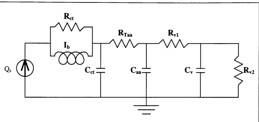
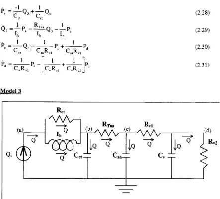
[image:32.562.58.501.115.516.2]

Model

3

Figure 2-14.

Model

3:

parallel

inertance

model

of

aortic arches and

conotruncus

with

Windkessel

afterload model.

By

continuity

we can write

the

constitutive

equations:

Qs

=

Qi

=

Q2

+

Q3

Q2

+

Q3

=

Q4

+

Q5

=

Q6

+

Q7

(33)

[image:33.562.70.492.50.617.2]

From

the elemental

equations

we can

write:

Pa-Pb=Q2Rct

b

xb

dt

Q3=-^-J(Pa-Pb)dt

HP

1

Q4=Cct^^Pb=-i-j-Q4dt

dt

PaTP"

R-Q5=^^

LTaa

Q6=Ca^=>R

Q7

=

dt

P

-P

c

rd

=_7^JQ6dt

R

Q8

=

cv

vl

dt

Pd=-l-jQ8dt

Q9=^

R

v2

Figure 2-15.

Model 3

block diagram.

(2.32)

(2.33)

(2.34)

(2.35)

(2.36)

(2.37)

(2.38)

(2.39)

K2-^

₀

Outport

ITinie.Qs]

Ql Q2

fc Ret ^ Pa-Pb

1

^

>

H3

From Workspace

Q3

zfcFl 04 f

^

\

Pb

RU

Q5 -<^j/Rtaa Pb-Pc

PTf-Llfl^

-trn

1/C^>

Pc -RLl f Q7 -<1/Rvl Pc-Pd t+m

^Ifl1^

-fcFl

Q

8 ,

1/Cv^>

Pd

::RU

Q9

"*k

(34)

Using

the

elemental

equations

(2.32-2.39)

in

the

continuity

equations we arrive at

the

following

state equations:

Q3=^LQ3+^LQs

(2.40)

^b

=

rrT~Pb+FlT-p<+^-Qs

(2-41>

*-ctKTaa

<~ctKTaa

<-ct

P=

l

P-c

r

b

^aa^Taa

P=-J_P-d

CR

<

1

+

Ca^Taa

^"aa^vl

Pc+TT-^Pd

C

R

(2-42)

1

+

v"-vl

L

v*^vl

*-v^-v2

Pd

(2.43)

2.1.6

Initial

Conditions

In

all simulation

methods,

there

exist

initial

conditions on

the

state

variables

of

the

system(s).

If

a

system

is starting

out

from

rest, the

initial

conditions can remain at

zero,

as

this

would

be

the

true

condition,

but

the

systems

in

this

study

are

already dynamic

and

have

been

so

for

a

long

time

(cardiovascular

activity;

the

heart is

the

first

functioning

organ).

Regardless

of

the

values given

to the

initial

conditions,

the

states should

eventually steady

out

to

the

conditions

dictated

by

the

model

in

a

simulation,

and given a

long

data

series, this

may

not

be

a problem

if

some of

the

data

during

the

start-up

period

of

the

simulation can

be

sacrificed.

The data in

this

study,

however,

is broken up

to

single

beats

or

cycles of cardiac

flow,

allowing virtually

no

time

for

"start-up"

of

the

simulation.

In

other

words, the

initial

conditions on

the

state

variables

in

the

simulation

must

represent

the

values of

the

states at a

point

midway (or

thereabouts)

in

a

single cardiac cycle.

Assigning

the

correct values

to the

initial

conditions

on

the

states

will

allow

the

model simulation

to

behave

as

if it had been

(35)

Fortunately,

the

initial

conditions can

be

computed

from

the

analytic state

equations.

If

we

use

the

first

few

values

of

input

flow, Qs,

(as

we

will

for

the simulations)

and

experimental

Pressure, Pa,

(this

is

the

output

of

the

simulations)

we

can

back-calculate

to

determine

what

the

state values should

be

at

the

beginning

of

the

simulation.

The

calculated

values

will

be

only

approximations since

differentiation

of

the

data

series

(finite

difference)

is

required

to

accommodate

the

analytic

expressions,

but

the

method

has

proved

to

be

sufficient

in

all

test

cases.

It

should also

be

noted

that the

initial

conditions on

the

states will

need

to

be

calculated

at each optimization

step

since

the

system parameter

values will

be

changing

from

(36)

2.2

Optimization

Techniques

2.2.1

Design Variables

In

any

optimization

problem

it is

necessary

to

specify

a set of

design

variables which

are used

to

find

the

solution

to the

problem.

The design

variables are used

in

the

calculation

of

the

objective

function,

and

in

some cases are

limited

by

constraint equations

(i.e.

equality,

inequality,

side).

The idea is

to

vary

the

design

variables

in

such

a

way

as

to

produce

minimization of

the

objective

function.

For

the

lumped

parameter circuit models presented

earlier, the

design

variables are

the

parameter values

(i.e.

Cct,

Rtaa,

Caa

etc.).

Two

scenarios will

be

entertained

with

regards

to

these

parameter values: constant parameter models and

linearly

varying

parameter models.

Constant

parameter models consist of a single

value

representing

the

parameter.

Linearly

varying

parameters consist of a constant

term

and a

term that

varies

linearly

with

the

input

flow,

Qs.

Constant Parameters

Linearly

Varying

Parameters

Rtaa

=

Rtaao

+

Rtaai*Qs

Cct

=

Ccto

+

Ccti*Qs

Caa

=

Caao

+

Caai

*Qs

Cv

=

Cv0

+

Cv,*Qs

Rvl

=Rvl0

+

Rvli*Qs

Rv2

=

Rv20

+

Rv2,

*Qs

lb

Ib

=

Ib0

+

Ibi*Qs

Ret

Rct

=

Rcto

+

Rcti*Qs

The

linearly

varying

parameter models

actually have

twice the

number

of

design

variables

as

do

the

constant

parameter

models

by

way

of

the

constant

term

in

addition

to the

coefficient on

the

linear

term.

This

"doubling"

of

design

variables

significantly

increases

the

(37)

2.2.2

The Method

of

Least

Squares

In

least

squares

optimization,

the objective

function

becomes

the

sum

_of

the

squared

differences between

the

model predicted and

experimental

data,

which would

be

the

pressure

at node

(a),

Pa,

for

all

three

models postulated

to

predict

blood flow.

If

we

refer

to

the

objective

function

as

F(x),

then the

optimization problem appears as:

/(x)

=

|Pa_experimentai-Pa

.predicted]

(differencing

equation)

(2.44)

m

min:

F(x)

= f(\)2 = /(x)r

/(x)

(objective

function)

(2.45)

i=\

Where

x

is

a vector of

the

design

variables of

length

n.

Numerous

optimization routines exist

for minimizing

the

sum-of-the-squares

in

such

an

application.

Most

methods

(i.e.

Steepest

Descent)

will require

the

computation of

the

gradient at

discrete

time

points with respect

to the

variables

in

order

to

determine

a search

direction

at a particular point.

The

gradient

is

typically

found

by determining

the

Jacobian

matrix with respect

to

the

design

variables and

incorporating

it in

the

following

expression:

VF(x)

=

27(x)r/(x)

(2.46)

The

Jacobian, J(x),

is

simply

a

matrix

of

the

first

partial

derivatives

of

the

differencing

equation

(2.43)

with

respect

to the

design

variables:

7(x)

=

[/(x)l

(Jacobian)

(2.47)

dxt

To

solve

for

the

gradient

of

F(x)

analytically, the

objective

function

must

be

written

in

a

closed

form in

terms

of

the

system parameters

(design

variables)

and

the

state variables.

Since

we

are

looking

at

multiple

time

points

in calculating

the

sum

of

the

squares,

the

(38)

function,

f(x),

is

not a single

value,

but

actually

an

array

of numbers.

When

the

difference is

squared,

we are

actually

performing

a

dot

product,

so

the

result

is

a

single valued objective

function

(see

equation

2.45).

The fact

that the

differencing

function, f(x),

contains multiple

points

implies

that the

Jacobian

matrix

is actually

vectorized.

That

is,

the

elements

of

the

Jacobian

matrix represent

the

first

partial

derivatives

with respect

to the

design

variables

at

multiple

time

points.

JT[f(*)]

=

<ti\_

#2.

<!f3_

<m

\dxx

dxx dxx

dx

\J

<%J_

%2_

j^3_

%jn

y

dx2 dx2 dx2

dx2

j

<%\

tfl

#3

ft

dx'dx/dx' '

dx,

n n n nJ

(n

design

variables,

m

time

points)

(2.48)

In

optimization

by

means

of

the

Steepest Descent

method, the

search

direction

is

calculated as

the

negative of

the

gradient.

By

equation

2.48

the

gradient

ends

up

being

a

vector with

n

elements,

the

same as

the

number of

design

variables.

SD

=

-VF(x)

(Search

Direction)

(2.49)

The

problem

is

then

turned

into

a

one-dimensional optimization problem with

the

introduction

of a

step

size,

a.

min:

F

(a)

= F(x'

+

a'

SD')

(2.50)

The

goal

is

to then

determine

a

step

size,

a*,

which will minimize

the

objective

function

at

the

current

values of

the

design

variables.

A

good method

for

determining

an

appropriate

step

size

is

the

Golden Section

search,

which uses

the

Golden

Ratio

to

reduce

the

interval

of

uncertainty

after

the

initial

bracketing

of

the

minimum

is

achieved.

The

interval

is

(39)

whole process

is iterated

until

convergence criteria

are

met,

or

until

some minimum

step

size

is

reached.

2.2.3

Numerical Optimization

Techniques

The

method

just described

requires analytic expressions

for

the

objective

function in

order

to

compute

the

search

directions.

For

simple

models,

this

is

a

relatively

simple

task,

assuming

we

have only

a

few design

variables.

MATLAB

contains a

"canned"

optimization

routine

specifically

catered

towards

least

squares minimization.

LEASTSQ

requires

a

call

to

an m-file

that

computes

the

objective

function based

upon

the

design

variables,

and

initial

conditions or

starting

values

for

these

variables.

The

computation of

the

search

directions

and

step

sizes are

all

contained within

the

canned routine.

While

the

LEASTSQ

routine

may

not

be specifically designed for

use

with

an objective

function

which

is

computed

through

the

simulation of a

dynamic linear

system,

it is

a numerical

method,

implying

that the

routine

should

be

general enough

to

handle

most optimizations problems

without

having

analytic

expressions

to

compute

the

gradients.

2.2.4

Verification

of

Optimization Techniques

To

test the

validity

and

performance

behind both

the

analytic

least

squares

method

and

the

canned

LEASTSQ

routine, the

circuit of

Model

1

was

used

as

a

test

case.

The

model

was

bread-boarded in

the

laboratory

and

the

circuit

was

driven

with

a

sinusoidal

current.

The

(40)

L

Rvi

AAA-y

U

c

v

16

Cct=10^f

RT=11.76kQ

Caa=10|if

Rv,=17.58kI2

C^lOnf

Rv2=H.78kfl

Cv:

Figure

2-16.

Benchtop

test

case

ofModel 1 using

electrical circuit.

Since

the

solving

of

the

state variables at each

iteration

of

the

optimization process

was

independent

of

the

optimization

technique

used,

both

tests

used

the

state

space

formulation

and

the

function LSIM

to

simulate

the

model.

This,

as

mentioned

before,

requires

that

we

develop

the

state

equations

for Model 1

.

By

continuity

we

can write

the

constitutive equations:

Is=ii

ii

=

b

+

i3

=

i4

+

is

=

ie

+

h

From

the

elemental

equations

we can

write:

=

Ca^-=>v.=J-fi2dt

ct

dt

C

J

h=-

Va"vb

R

i-i

=Ca

Taa

dvv

dt

-F-JMt

vb-vc

[image:40.562.66.507.51.279.2]

(41)

dv

?"/'.*

1-,

=

7"r

v2

Using

the

elemental

equations

in

the

continuity

equations we arrive at

the

following

state

equations:

1

C,RT

'

C,RT,a

C

cti,LTaa '

ctixTaa

Vb

=

^-aa^-Taa

V,

-+

^aa^Taa

^aaRvl

vb

+

CaaRvl

V

=

Rv,cv

Vb

n

l

+

R.i

_vl

R

x>-v2

To simplify

matters,

we will

only

use

Cct, C^,

and

RTaa

as

the

design

variable.

Letting

va

be

the

desired

output,

the