Sensitivity of fine scale species distribution models to locational uncertainty in occurrence data across multiple sample sizes

Sensitivity of fine-scale species distribution models to

locational uncertainty in occurrence data across multiple

sample sizes

Peter J. Mitchell

*, Jacquomo Monk

and Laurie Laurenson

1_{Centre for Integrative Ecology, School of Life and Environmental Sciences, Deakin University, PO Box 423, Warrnambool,}

Vic. 3280, Australia;2Centre for Environment, Fisheries and Aquaculture Science, Pakefield Road, Lowestoft, Suffolk NR33 0HT, UK; and3Institute for Marine and Antarctic Studies, University of Tasmania, Private Bag 49, Hobart, Tas. 7001, Australia

Summary

1. To generate realistic predictions, species distribution models require the accurate coregistration of occurrence data with environmental variables. There is a common assumption that species occurrence data are accurately georeferenced; however, this is often not the case. This study investigates whether locational uncertainty and sample size affect the performance and interpretation of fine-scale species distribution models.

2. This study evaluated the effects of locational uncertainty across multiple sample sizes by subsampling and spatially degrading occurrence data. Distribution models were constructed for kelp (Ecklonia radiata), across a large study site (680 km2_{) off the coast of southeastern Australia. Generalized additive models were used to}

pre-dict distributions based on fine-resolution (25 m cell size) seafloor variables, generated from multibeam echo-sounder data sets, and occurrence data from underwater towed video. The effects of different levels of locational uncertainty in combination with sample size were evaluated by comparing model performance and predicted distributions.

3. While locational uncertainty was observed to influence some measures of model performance, in general this was small and varied based on the accuracy metric used. However, simulated locational uncertainty caused changes in variable importance and predicted distributions at fine scales, potentially influencing model interpre-tation. This was most evident with small sample sizes.

4. Results suggested that seemingly high-performing, fine-scale models can be generated from data containing locational uncertainty, although interpreting their predictions can be misleading if the predictions are interpreted at scales similar to the spatial errors. This study demonstrated the need to consider predictions across geographic space rather than performance alone. The findings are important for conservation managers as they highlight the inherent variation in predictions between equally performing distribution models, and the subsequent restrictions on ecological interpretations.

Key-words: georeferencing error, habitat suitability, model performance, occurrence data accuracy, spatial error

Introduction

Species distribution models (SDMs) have been used widely in biogeography to characterize the ecological niche of species and to predict the geographic distribution of their habitat (Elith et al. 2006; Araujo & Peterson 2012). Despite their increasing use, SDMs pose many conceptual problems (Jimenez-Valverde, Lobo & Hortal 2008; Soberon & Naka- mura 2009) and encompass many methodological uncertain-ties (Barry & Elith 2006; Heikkinenet al.2006; Rocchiniet al. 2011).

A fundamental challenge in using SDMs is the uncertainty around where an observation is located, and is known as

locational or positional uncertainty. Past studies into the effects of locational uncertainty have primarily focussed on simulating the errors occurring in existing data sets held in museums and herbaria, which are increasingly accessible through Internet portals (e.g. Global Biodiversity Information Facility; Chapman 2005). These studies have been motivated by the fact that the majority of existing observation data sets were collected before the popularization of GPS technology. When these records were digitized, geographic coordinates were often inferred from textual descriptions and may be sub-stantially incorrect (Wieczorek, Guo & Hijmans 2004; Feeley & Silman 2010). Similarly, contemporary marine samples may have been positioned using outdated technology, such as the Decca navigation system, and may have positional errors on the order of hundreds of metres (Last 1992; Kubicki & Diesing 2006). This problem becomes important when the observation

*Correspondence author. E-mail: [email protected]

data are used to develop SDMs, as coordinates are used to extract the colocated environmental variables. Accordingly, locational uncertainty will transfer to inaccurate characteriza-tions of the species–environment relationship (Feeley & Silman 2010).

Although not widely recognized, observation data col-lected using modern positioning systems invariably contain locational uncertainty. For example, the current locational accuracy of most standard GPS units can be~30 m (Frair et al. 2010). While this is small compared to those con-tained in digitized records, when these data sets are incor-porated into a fine-scale SDM framework, this minor locational error affects the accuracy of model predictions (Guisan et al. 2007). With technological advances in the collection of environmental data sets, SDMs are being built at increasingly finer resolutions, not more so than in the marine environment, where multibeam echosounders (MBESs), along with other techniques, are now capable of providing seafloor structure information at resolutions of <2 m (Brown et al. 2011). Consequently, locational uncer-tainty continues to be problematic despite the development of improved positioning systems (Rigby, Pizarro & Wil-liams 2006). In a recent study, Rattrayet al. (2014) quanti-fied the propagated error associated with each component of underwater camera positioning (a technique commonly used to collect observation data in marine ecosystems). They found a linear increase in location error with camera depth, equating to a 15 m horizontal error near the surface and 57 m error at a depth of 100 m. This suggests that the maximum error in location of a species observation may often exceed the resolution of the predictor data sets, and, thus, locational uncertainty remains an issue with data sets collected using modern positioning systems.

Statistical techniques have been developed to estimate the locational uncertainty in occurrence data and remove highly uncertain observations prior to analysis (Wieczorek, Guo & Hijmans 2004; Guo, Liu & Wieczorek 2008). Taking such an approach, however, ultimately reduces the sample size, which in turn decreases model accuracy (Hernandez et al. 2006). Accordingly, having locational uncertainty in observation data should not automatically be a reason to discard the data (Chapman 2005). In this case, it is important to know whether and where this locational uncertainty is problematic. For example, Grahamet al.(2008) compared different SDMs to see whether they were affected by an introduced random error (up to 5 km) to the location of their observation data. Although they concluded that SDMs are, in general, robust to locational uncertainty at broad scales, recent studies argue that this is not consistent. For example, Hefley et al. (2014) observed that locational errors could bias their models and rec-ommended correcting for locational errors where possible. Consequently, there is a clear need for further investigation into locational uncertainty, especially using finer resolution data sets.

The sample sizes used to generate models vary enor-mously between studies. While a larger data set is always preferred, the difficulty of sampling rare or cryptic species

means samples are inherently limited. It is also widely regarded that predictive performance of models improves, and variation between predictive accuracy decreases, with larger data sets (e.g. Pearce & Ferrier 2000; Hernandez et al. 2006; Wisz et al. 2008). When sample size is small, outliers have a stronger influence on the fit of a model (Wisz et al. 2008). Considering locational error is antici-pated to create outliers in the data, it is logical to expect that locational error will affect model performance more when coefficients are derived from smaller sample sizes. However, no study has compared how model performance is influenced by varying sample size with data containing locational errors.

The objectives of this study are to evaluate the extent to which locational uncertainty within observation data influ-ences the performance and interpretation of fine-scale SDMs. This is examined across multiple sample sizes to determine whether these effects vary as a result of the number of observa-tions used to generate the model. As SDMs are increasingly being applied to finer scale data sets, this paper provides a timely investigation into the potential effects of locational uncertainty on fine-scale SDMs.

Materials and methods

STUDY S IT E

The study site consisted ofc.135 km of coastline around Cape Otway, in southeastern Australia. The site extended from the western bound-ary of the Twelve Apostles Marine National Park, to the coastal waters south of Anglesea (Fig. 1). A total of 680 km2_{of seafloor were} sur-veyed with depth ranging from 6 to 79 m. The site consists of sandy sediment with a number of high relief reef systems increasing in sand inundation with depth. Species assemblages are complex and highly diverse (Phillips 2001), with kelpPhyllospora comosa(C. Agardh) and Ecklonia radiata(C. Agardh) dominant in shallower waters.

S E A F L O O R I N F O R M A T I O N A C Q U I S IT IO N A N D P R O C E S S IN G

Seafloor structure variables were derived from MBES data sets. The MBES data were acquired using a hull-mounted Reson Seabat 8101 (240 kHz) MBES over a series of field campaigns between November 2005 and December 2007 (Ierodiaconouet al.2007b). Positioning was achieved using a real-time differential GPS (030 m horizontal accu-racy) with an integrated Positioning and Orientation system for Marine Vessels, to correct for heave, pitch, roll and yaw (002°accuracy) (Monket al.2011). Survey lines were spaced to ensure a 50% overlap of sonar coverage, allowing erroneous data points to be cleaned. Data were corrected to lowest astronomical tide datum, and a bathymetric grid at 1-m cell resolution (125 mm vertical accuracy) was generated (a detailed description of the MBES data processing is provided in Rat-trayet al.2009). The MBES bathymetry and backscatter data sets were resampled to a 25-m cell resolution for analysis.

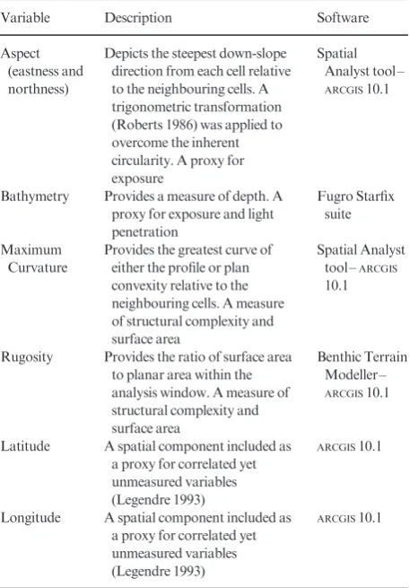
2009, 2013). Variables were calculated inARCGIS10.1 (ESRI) using an analysis window of 393 cells. Backscatter and slope were removed following the test for correlated variables (Spearman’s q>07, Appendix S1, Supporting information), and the remaining variables were included in all models (Table 1).

In addition to the seafloor structure variables, spatial variables of longitude and latitude were included as predictor variables to account for regional trends in spatial variation (Borcard, Legendre & Drapeau 1992; Legendre 1993; Guisan & Thuiller 2005) (Appendix S1).

O B S E R V A T ION D A T A

The kelp speciesE. radiatawas selected for modelling as it is dominant in the study area. It is known to exhibit a strong relationship with sea-floor characteristics (Rattrayet al.2009; Ierodiaconouet al.2011) and was readily discernible in the video data, thus reducing potential effects of imperfect detection (Monket al.2012; Monk 2014).E. radiatawas surveyed using towed video transects. Following a visual inspection of the bathymetry, 45 towed video transects covering 176 km of seafloor were performed, predominantly perpendicular to the coast, to encompass the main physical gradients.

Video data were collected using a remotely operated vehicle (VideoRay Pro 3, VideoRay LLC, Phoenixville, PA, USA.) towed at 05–1 ms 1(1–2 km). Through the use of a winch system and real-time video, the camera was maintained~2 m from seafloor, providing con-tinuous coverage in a field of view of~3–5 m along each transect. An ultra-short baseline transponder was attached to the video unit to allow three-dimensional positioning of the unit relative to the vessel-mounted differential GPS (for further details see Rattrayet al.2014).

Video data were collected across three survey periods between Jan-uary 2006 and March 2007. Video samples were classified to the Victo-rian Towed Video Classification Program (Ierodiaconouet al.2007b). This scored video data were cleaned to remove invalid frames due to

Fig. 1.Study site location.

Table 1. Derivative products from MBES, retained after correlation test

Variable Description Software

Aspect (eastness and northness)

Depicts the steepest down-slope direction from each cell relative to the neighbouring cells. A trigonometric transformation (Roberts 1986) was applied to overcome the inherent circularity. A proxy for exposure

Spatial Analyst tool–

ARCGIS10.1

Bathymetry Provides a measure of depth. A proxy for exposure and light penetration

Fugro Starfix suite

Maximum Curvature

Provides the greatest curve of either the profile or plan convexity relative to the neighbouring cells. A measure of structural complexity and surface area

Spatial Analyst tool–ARCGIS

10.1

Rugosity Provides the ratio of surface area to planar area within the analysis window. A measure of structural complexity and surface area

Benthic Terrain Modeller_–

ARCGIS10.1

Latitude A spatial component included as a proxy for correlated yet unmeasured variables (Legendre 1993)

ARCGIS10.1

Longitude A spatial component included as a proxy for correlated yet unmeasured variables (Legendre 1993)

ARCGIS10.1

poor visibility, and then, the presence/absence of E. radiata was extracted.

Autocorrelation was anticipated due to the use of continuous video data. To determine at what distance autocorrelation was influencing model fit, generalized additive models (GAMs) were produced using the full data set and autocorrelation in the residuals was interrogated (Dormann et al.2007). Following assessment of autocorrelation of model residuals (Appendix S2), ground truth samples were thinned by applying a minimum distance of 150 m between samples to reduce this effect. While statistical methods are available to control for autocorre-lation rather than delete valuable data (Dormannet al.2007), in this case data thinning was selected so as to allow a more commonly used modelling approach to be applied. Further, after thinning, our data still contained a total observation data set of 896 points.

DA T A T RE A T ME N T

Sample size

Bootstrap sampling with replacement was performed to provide multiple smaller replicate data sets from the original complete data set of 896 points. For each replicate, a random sample of 200 points was set aside as a testing sample. A training sample (points used to build the prediction model) was then randomly selected from the remaining points. This division of sample data was repeated to create ten replicates for each sample size. Training sam-ple sizes were made up of 100, 200 and 400 points, with all models tested against a sample size of 200 points.

Simulated locational uncertainty

Six levels of locational uncertainty were simulated in the occurrence data by moving points randomly from their original location. Loca-tional uncertainty was simulated by creating a buffer around each point location representing the simulated error, then randomly gen-erating a point within that circle. Where sample points occurred near the study region’s boundaries, the locational uncertainty buffer was clipped to this boundary to restrict sample movement to within the study site. This meant that each point was individually moved in a random direction, by a random distance up to the potential propagated error. The assumption of a circular radius of uncer-tainty is generally reasonable (Visscher 2006; Graham et al.2008). In addition to control data sets, where point locations were unper-turbed, the error treatments were 5, 25, 50, 200 and 400 m. The magnitude of error simulated in this study reflects the possible range of error that may be occurring during various sample tech-niques. While the smallest error margins are comparable to what might occur using modern positioning systems (Rattrayet al.2014), locational uncertainty up to 400 m has been reported in historical data sets, such as where the Decca navigation system was used for positioning (Last 1992; Kubicki & Diesing 2006).

M O DELLIN G APPROACH

Generalized additive models were used to fit presence/absence data to the seafloor variables for each treatment and replicate. GAMs are like-lihood-based regression models, fitting nonparametric, data-defined smoothers to create nonlinear functions (Hastie & Tibshirani 1986). GAMs have been used for SDMs and have been shown to perform rea-sonably well compared with other presence_–absence methods (Elith

et al.2006). The GAMs were implemented inRusing the package ‘mgcv’ (Wood & Augustin 2002) using default settings with smoothing parameters selected using restricted maximum likelihood (Venables & Ripley 2002). A log-transformation was applied to rugosity. To main-tain the aim of parsimonious model building, no interaction terms between variables were included in the models (Mellertet al.2011). Models were then output as continuous suitability maps and also reclassified into Boolean (presence/absence) predictions using the average probability/suitability approach (Liuet al.2005).

MO DEL EVALUATION

A comprehensive evaluation of how locational uncertainty and sample size affect habitat suitability models requires the comparison of model interpretation as well as model performance (e.g. Barry & Elith 2006). Therefore, models were compared in terms of performance and model prediction.

Model performance

Models were assessed using the corresponding evaluation data with-held for each replicate. Since no single method fully summarizes model performance, models were evaluated with six recommended methods (Fielding & Bell 1997; Lobo, Jimenez-valverde & Real 2008). Metrics included the following: percentage correctly classified (PCC), correctly predicted positive fraction (sensitivity), correctly predicted negative fraction (specificity), area under curve (AUC) of the receiver operating characteristic (Fielding & Bell 1997) and kappa (Cohen 1960). AUC was calculated from the continuous suitability map while the threshold-dependent performance metrics (PCC, sensitivity, specificity and kappa) were calculated from the Boolean prediction. Explained deviance (d2_{) of each model was also} compared as a measure of the training data closeness of fit, taking into account the number of degrees of freedom (Engler, Guisan & Rechsteiner 2004).

As this was a simulation study, it was deemed inappropriate to per-form hypothesis tests to examine statistical significance. In simulation studies where models are known to be different, a frequentist approach usingP-values merely indicates whether a sufficient number of simula-tions were run to detect an effect (Whiteet al.2014). Rather, the focus is on the magnitude of variation between simulations.

Model prediction

Results

IN FLU E NCE OF LOCAT ION AL UN CERT AIN TY A ND S A M P L E S IZ E ON M O D E L PE R F O R M A N C E

Locational uncertainty had limited effect on model perfor-mance (Fig. 2). Boxplots for AUC, PCC, sensitivity, specificity and kappa show that models of the same sample size derived from data containing locational error performed as well as those containing no error. While there is some variation in measured model performance as a result of incorporating loca-tional error, there does not appear to be a general trend, and even at 400 m, the effect was minimal. The exception was explained deviance which decreased relative to the control when simulated error was≥200 m.

The effects of sample size on model performance were more pronounced, with larger sample sizes producing more accurate models (Fig. 2). In addition, there was less variation in model performance within treatment observed when sample size was large. This trend was observed for AUC, kappa, PCC and sen-sitivity. Nevertheless, the effect was small and boxplots show overlap in measured accuracy between sample sizes. Explained deviance and specificity were the exceptions, with little or no discernible change observed with increasing sample size.

IN FLU E NCE OF LOCAT ION AL UN CERT AIN TY A ND S A M P L E S IZ E ON M O D E L INT E R P R ET A T I O N

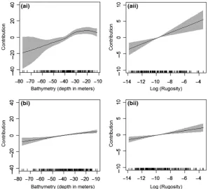
Although locational uncertainty had a limited effect on mea-sured performance, the relative influence of the predictor vari-ables differed between models. Generally, the major predictor variables for all models were bathymetry, rugosity, longitude and latitude (Appendix S3). However, the response curves of fitted coefficients varied as a result of incorporating locational uncertainty into the data (Fig. 3). For some variables, only the magnitude of the relationship changed as a result of locational uncertainty (Fig. 3aii, bii). Other variables showed more note-worthy differences with the relationship along the environmen-tal gradient changing altogether (Fig. 3ai, bi). This was supported by analysis of rank importance of predictor vari-ables, which observed changes in variable importance as a result of uncertainty treatments, particularly when sample size was small (Appendices S3 and S4).

IN FLU E NCE OF LOCAT ION AL UN CERT AIN TY A ND S A M P L E S IZ E ON M O D E L PR E D I C T IO N S

Despite similar model performance, differences in model pre-dictions were observed between simulated uncertainty

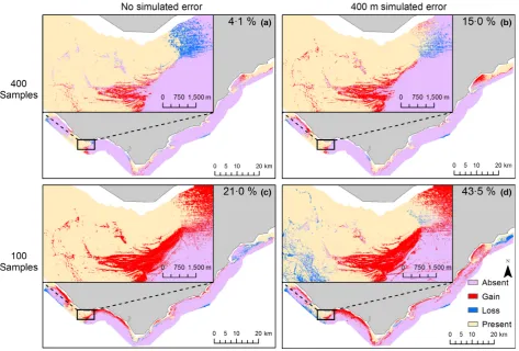
treatments and models containing no simulated locational error (Fig. 4). Models generated from spatially degraded data 200 m or greater were observed to predict a larger area of suit-able habitat compared with predictions from models contain-ing no simulated locational error (Fig. 5b). However, when locational error was ≤50 m, there was little or no effect. In addition, there was no discernible effect of uncertainty treat-ments on presence agreement (Fig. 5a). Generally, locational uncertainty resulted in subtle differences in predictions for large sample sizes, such as the interface between reef and sedi-ment (Fig. 4a,b). Predictions developed from smaller training samples showed a greater degree of variation as a result of locational uncertainty with differences visible at both local and regional scales (Fig. 4c,d).

The effects of sample size on model predictions were more noticeable. As sample size decreased, increased variation between replicates was observed in the presence agreement and extent of suitable habitat predicted (Fig. 5a,b). Generally, the area of presence agreement decreased with decreasing sample sizes (Fig. 5a). Similarly, differences in the total area predicted as suitable were also observed between sample sizes (Fig. 5b), with a greater area predicted as suitable when sample sizes were smaller.

Discussion

The precision in the spatial locality of occurrence data is thought to be of critical importance for the development of SDMs (Naimi et al. 2011). The occurrence data used to fit such models are known to lead to differences in SDM pre-dictions, thus expected to affect their performance (Guisan et al. 2007; Osborne & Leit~ao 2009). However, as shown here, the importance of locational uncertainty is often

dwarfed when compared with other factors affecting SDM predictions (i.e. sample size). Indeed, variation in locational uncertainty had relatively small effects on the performance and the ecological interpretations based on SDMs, particu-larly at uncertainty scales ≤50 m. This may in part be explained by spatial autocorrelation. Original assessments characterized spatial autocorrelation in the presence/absence ofE. radiatato be present up to a distance of 150 m. Spa-tial dependence implies a higher similarity for any two data points which are <150 m apart. It follows logically that moving one data point any distance less than this from the true location will effectively remain in the same sample and have limited effect on the model.

Model performance consistently increased with sample size for all data sets. However, the effects of locational uncertainty on model performance were less evident, with boxplots only indicating that certain measures were affected (PCC, speci-ficity, kappa and explained deviance), but not others (AUC and sensitivity). Further, when locational uncertainty was on the scales expected with current positioning systems (Rattray et al.2014), no discernible effect of model performance was observed. These findings therefore support those of Graham et al. (2008) and Osborne & Leit~ao (2009), that occurrence data containing locational uncertainty can provide high-per-forming models. However, it may be worth considering the effects of locational uncertainty when errors are expected to be in the range of 200–400 m, such as in historical data sets posi-tioned using outdated technologies. While model performance was generally robust to locational error of this magnitude, sug-gesting the suitability of using data sets known to contain error, explained deviance was observed to decrease and models containing error tended to overestimate the distribution of suitable habitat.

An important distinction between the current and most pre-vious studies is the finding that locational uncertainty has the potential to affect the relative influence of predictor variables and the predictions from these models, which was pronounced when sample sizes were small. This has implications for model inference, as distributions generated from data sets containing fine-scale locational uncertainty may differ as a result of the errors. These results are supported by Osborne & Leit~ao (2009), suggesting that while useful predictions may be gener-ated from data containing locational uncertainty, ecological interpretations must consider the uncertainty introduced through that error. This is particularly evident when the scale of concern is small, such as when areas within the study site are of particular importance, or when interpreting factors that may influence distribution.

This study found that with increasing sample size, model performance increased and variation in predictive accuracy decreased. Larger sample sizes performed better across all per-formance metrics except specificity and explained deviance, which showed no noticeable change. This link between sample size and model performance is well established in the existing literature (Pearce & Ferrier 2000; Hernandezet al.2006; Wisz et al.2008). However, with the exception of Hernandezet al.

(2006), these studies have not compared how sample size affects the spatial prediction from the models. Similar to Her-nandez et al. (2006), spatial predictions compared between sample sizes found that as sample size increased, there was greater spatial similarity to the complete data set model. The results also highlighted that smaller sample sizes tend to predict larger regions of suitable habitat. However, variation in spatial predictions is also increased with smaller sample sizes. This supports the expectation that a greater number of samples pro-vide a more representative sample of the environmental space and are therefore likely to more accurately define the parame-ters (Carroll & Pearson 1998). While model performance has typically been investigated relative to sample sizes<100 (Her-nandezet al. 2006; Wiszet al.2008), this study found that samples sizes as large as 400 points differed in model perfor-mance, if only marginally. Despite the observed decrease in model performance, none of the models would be rejected on this basis (according to thresholds for satisfactory models based on AUC–Swets 1988; Pearce & Ferrier 2000; Graham et al.2008).

This study demonstrates the need to not only consider model performance but also the spatial predictions when com-paring different models. Numerous studies have compared

modelling approaches based only on performance metrics (Segurado & Araujo 2004; Elithet al.2006; Tsoaret al.2007; Grahamet al.2008), yet models of similar performance can produce very different geographic predictions (Hernandez et al. 2006; Monk et al. 2012). Here, models classified the majority of habitat accurately regardless of sample size or uncertainty treatment (AUC>08). Despite high perfor-mance, variation was observed between geographic predictions particularly at the fringe of optimal habitat (i.e. forE. radiata the transition from reef to sediment). For example, an increase in predicted suitable habitat of 150% (Fig. 4b) may be reliable from a modelling perspective; however, in real terms for this study area, this equates to an over prediction ofc.21 km2of suitable habitat due to the use of degraded data. The rank importance of predictor variables and fitted coefficients tell a similar story. Variation in the relative importance of predictor variables and fitted coefficients is present between sample sizes and uncertainty treatment groups. Thus, while predictive suc-cess may be retained, the ecological interpretation of the fac-tors determining a species distribution would differ depending on sample size and uncertainty treatment. The value of these models is therefore dependent on their desired purpose. While they may provide useful information across the site as a whole, interpretation of ecological processes or localized distributions, such as areas of fringe habitat, can be misleading (Graham et al. 2008; Johnson & Gillingham 2008; Osborne & Leit~ao 2009).

The results of this study have a number of implications for future species distribution modelling at fine scales. The most obvious recommendation is the value of increasing sample size where available, to better inform models. This must be balanced by data availability and the time-consum-ing process of its accurate classification (Rattrayet al.2014).

In some cases, the benefit of increasing spatial accuracy may be outweighed by the costs and requirements of an improved positioning system (Rattrayet al.2014). However, this study suggests it may be more beneficial to focus on increasing survey effort rather than further reducing locational uncer-tainty when building fine-scale SDMs. Researchers must determine the acceptable level of locational uncertainty within their data based on the aims of their study and tools available, allowing them to address these during the plan-ning stage (Rattray et al. 2014). Understanding how loca-tional uncertainty can affect the interpretation of predicted distributions may determine the necessary scale for mod-elling a particular species (Guisan et al. 2007; Osborne & Leit~ao 2009).

In summary, this study has explored how locational error in occurrence data influences model performance and spatial pre-dictions in fine-scale SDMs. By subsampling and spatially degrading occurrence data beyond what is reasonable, this study evaluated the effects of locational error across multiple sample sizes. The results indicated that while sample size affects model performance, the effects of fine-scale locational error were generally minimal regardless of sample size. This is encouraging as it indicates that accurate fine-scale models can be generated from data positioned using imprecise methods, such as historical data sets. However, while the effects of loca-tional error on measures of model performance were small, there was variation in variable importance use and spatial pre-dictions from the models. This highlights the need to consider predictions across geographic space rather than model perfor-mance alone. These findings are important for conservation managers as they highlight the inherent variation between equally high performing distribution models, and the subse-quent restrictions on ecological interpretations.

Fig. 5. (a) Boxplot of the presence agreement between subsampled and simulated error treatments compared with the complete data set model. Columns indicate the variation within each treatment, grouped by sample size. A 1% decrease in presence agreement equates toc.14 km2_of

Acknowledgements

The authors would like to thank Deakin University, the Coastal CRC, Parks Victoria, Fugro and DSE for access to the towed video and MBES data sets that were collected as part of the Victorian Marine Habitat Mapping Project. Thanks to Steffan Howe from Parks Victoria for providing the data used in this study. Thanks to the crews aboardCourageous II andBluefin for the assistance in the collection of the towed video and MBES data sets. Analyses were undertaken at Deakin University, Warrnambool, Victoria, GIS Labora-tory facility. J.M. was supported by the Marine Biodiversity Hub through funding from the Australian Government’s National Environmental Science Program (NESP), administered by the Department of the Environment. NESP Marine Biodiversity Hub partners include the Institute for Marine and Antarctic Studies, University of Tasmania; CSIRO, Geoscience Australia, Australian Institute of Marine Science, Museum Victoria, Charles Darwin University and the University of Western Australia.

Data accessibility

The MBES and video data are restricted access and owned by the Victorian Government. Requests to archive data were denied. Metadata has been lodged for the data via Deakin Research Online (http://dro.deakin.edu.au/view/ DU:30043228).

References

Araujo, M.B. & Peterson, A.T. (2012) Uses and misuses of bioclimatic envelope modeling.Ecology,93, 1527–1539.

Barry, S. & Elith, J. (2006) Error and uncertainty in habitat models.Journal of Applied Ecology,43, 413–423.

Borcard, D., Legendre, P. & Drapeau, P. (1992) Partialling out the spatial compo-nent of ecological variation.Ecology,73, 1045–1055.

Brown, C.J., Smith, S.J., Lawton, P. & Anderson, J.T. (2011) Benthic habitat mapping: a review of progress towards improved understanding of the spatial ecology of the seafloor using acoustic techniques.Estuarine, Coastal and Shelf Science,92, 502–520.

Carroll, S.S. & Pearson, D.L. (1998) The effects of scale and sample size on the accuracy of spatial predictions of Tiger Beetle (Cicindelidae) species richness. Ecography,21, 401–414.

Chapman, A.D. (2005).Uses of Primary Species-Occurrence Data, version 1.0. Copenhagen. Global Biodiversity Information Facility.

Cohen, J. (1960) A coefficient of agreement of nominal scales.Educational and Psychological Measurement,20, 37–46.

Dormann, C.F., McPherson, J.M., Araujo, M.B., Bivand, R., Bolliger, J., Carl, G.et al.(2007) Methods to account for spatial autocorrelation in the analysis of species distributional data: a review.Ecography,30, 609–628.

Elith, J., Graham, C.H., Anderson, R.P., Dudik, M., Ferrier, S., Guisan, A.et al. (2006) Novel methods improve prediction of species’ distributions from occur-rence data.Ecography,29, 129–151.

Engler, R., Guisan, A. & Rechsteiner, L. (2004) An improved approach for pre-dicting the distribution of rare and endangered species from occurrence and pseudo-absence data.Journal of Applied Ecology,41, 263–274.

Feeley, K.J. & Silman, M.R. (2010) Modelling the responses of Andean and Amazonian plant species to climate change: the effects of georeferencing errors and the importance of data filtering.Journal of Biogeography,37, 733–740. Fielding, A.H. & Bell, J.F. (1997) A review of methods for the assessment of

pre-diction errors in conservation presence/absence models.Environmental Conser-vation,24, 38–49.

Frair, J.L., Fieberg, J., Hebblewhite, M., Cagnacci, F., DeCesare, N.J. & Ped-rotti, L. (2010) Resolving issues of imprecise and habitat-biased locations in ecological analyses using GPS telemetry data.Philosophical Transactions of the Royal Society of London Series B, Biological Sciences,365, 2187–2200. Graham, C.H., Elith, J., Hijmans, R.J., Guisan, A., Peterson, A.T., Loiselle, B.A.

et al.(2008) The influence of spatial errors in species occurrence data used in distribution models.Journal of Applied Ecology,45, 239–247.

Guisan, A. & Thuiller, W. (2005) Predicting species distribution: offering more than simple habitat models.Ecology Letters,8, 993–1009.

Guisan, A., Graham, C.H., Elith, J., Huettmann, F., Dudk, M., Ferrier, S.et al. (2007) Sensitivity of predictive species distribution models to change in grain size.Diversity and Distributions,13, 332–340.

Guo, Q., Liu, Y. & Wieczorek, J. (2008) Georeferencing locality descriptions and computing associated uncertainty using a probabilistic approach.International Journal of Geographical Information Science,22, 1067–1090.

Hastie, T. & Tibshirani, R. (1986) Generalized additive models. Statistical Science,1, 297–318.

Hefley, T.J., Baasch, D.M., Tyre, A.J. & Blankenship, E.E. (2014) Correction of location errors for presence-only species distribution models.Methods in Ecol-ogy and Evolution,5, 207–214.

Heikkinen, R.K., Luoto, M., Araujo, M.B., Virkkala, R., Thuiller, W. & Sykes, M.T. (2006) Methods and uncertainties in bioclimatic envelope modelling under climate change.Progress in Physical Geography,30, 751–777. Hernandez, P.A., Graham, C.H., Master, L.L. & Albert, D.L. (2006) The effect

of sample size and species characteristics on performance of different species distribution modeling methods.Ecography,29, 773–785.

Ierodiaconou, D., Laurenson, L., Burq, S. & Reston, M. (2007a) Marine ben-thic habitat mapping using Multibeam data, georeferencedvideo and image classification techniques in Victoria, Australia.Journal of Spatial Science,52, 93–104.

Ierodiaconou, D., Rattray, A.J., Laurenson, L., Monk, J. & Lind, P. (2007b). Vic-torian marine habitat mapping project. Report to Department of Environ-ment, Deakin University, Australia, 1–210.

Ierodiaconou, D., Monk, J., Rattray, A.J., Laurenson, L. & Versace, V.L. (2011) Comparison of automated classification techniques for predicting benthic bio-logical communities using hydroacoustics and video observations.Continental Shelf Research,31, 28–38.

Jimenez-Valverde, A., Lobo, J.M. & Hortal, J. (2008) Not as good as they seem: the importance of concepts in species distribution modelling.Diversity and Distributions,14, 885–890.

Johnson, C.J. & Gillingham, M.P. (2008) Sensitivity of species-distribution mod-els to error, bias, and model design: an application to resource selection func-tions for woodland caribou.Ecological Modelling,213, 143–155.

Kubicki, A. & Diesing, M. (2006) Can old analogue sidescan sonar data still be useful? An example of a sonograph mosaic geo-coded by the DECCA naviga-tion system.Continental Shelf Research,26, 1858–1867.

Last, D. (1992) The accuracy and coverage of Loran-C and of the Decca Naviga-tor System–and the fallacy of fixed errors.The Journal of Navigation,45, 36–51.

Legendre, P. (1993) Spatial autocorrelation: trouble or new paradigm?Ecology, 74, 1659–1673.

Liu, C., Berry, P.M., Dawson, T.P. & Pearson, R.G. (2005) Selecting thresholds of occurrence in the prediction of species distributions.Ecography,28, 385– 393.

Lobo, J.M., Jimenez-valverde, A. & Real, R. (2008) AUC: a misleading measure of the performance of predictive distribution models.Global Ecology and Bio-geography,17, 145–151.

Mellert, K.H., Fensterer, V., Kuchenhoff, H., Reger, B., K€ €olling, C., Klemmt, H.J. & Ewald, J. (2011) Hypothesis-driven species distribution models for tree species in the Bavarian Alps.Journal of Vegetation Science, 22, 635–646.

Monk, J. (2014) How long should we ignore imperfect detection of species in the marine environment when modelling their distribution?Fish and Fisheries,15, 352–358.

Monk, J., Ierodiaconou, D., Bellgrove, A., Harvey, E.S. & Laurenson, L. (2011) Remotely sensed hydroacoustics and observation data for predicting fish habi-tat suitability.Continental Shelf Research,31, 17–27.

Monk, J., Ierodiaconou, D., Harvey, E.S., Rattray, A.J. & Versace, V.L. (2012) Are we predicting the actual or apparent distribution of temperate marine fishes?PLoS One,7, 1–11.

Naimi, B., Skidmore, A.K., Groen, T.A. & Hamm, N.A.S. (2011) Spatial auto-correlation in predictors reduces the impact of positional uncertainty in occur-rence data on species distribution modelling.Journal of Biogeography,38, 1497–1509.

Osborne, P.E. & Leit~ao, P.J. (2009) Effects of species and habitat positional errors on the performance and interpretation of species distribution models.Diversity and Distributions,15, 671–681.

Pearce, J. & Ferrier, S. (2000) Evaluating the predictive performance of habitat models developed using logistic regression.Ecological Modelling,133, 225– 245.

Phillips, J.A. (2001) Marine macroalgal biodiversity hotspots: why is there high species richness and endemism in southern Australian marine benthic flora? Biodiversity and Conservation,10, 1555–1577.

Pontius, R.G., Shusas, E. & McEachern, M. (2004) Detecting important categori-cal land changes while accounting for persistence.Agriculture, Ecosystems and Environment,101, 251–268.

Rattray, A.J., Ierodiaconou, D., Monk, J., Versace, V.L. & Laurenson, L. (2013) Detecting patterns of change in benthic habitats by acoustic remote sensing. Marine Ecology Progress Series,477, 1–13.

Rattray, A.J., Ierodiaconou, D., Monk, J., Laurenson, L. & Kennedy, P. (2014) Quantification of spatial and thematic uncertainty in the application of under-water video for benthic habitat mapping.Marine Geodesy,37, 315–336. Rigby, P., Pizarro, O. & Williams, S.B. (2006). Towards geo-referenced AUV

navigation through fusion of USBL and DVL measurements.Oceans 2006. 1–6

Roberts, D.W. (1986) Ordination on the basis of fuzzy set theory.Vegetatio,66, 123–131.

Rocchini, D., Hortal, J., Lengyel, S., Lobo, J.M., Jimenez-valverde, A., Ricotta, C., Bacaro, G. & Chiarucci, A. (2011) Accounting for uncertainty when map-ping species distributions: the need for maps of ignorance.Progress in Physical Geography,35, 211–226.

Segurado, P. & Araujo, M.B. (2004) An evaluation of methods for modelling spe-cies distributions.Journal of Biogeography,31, 1555–1568.

Soberon, J. & Nakamura, M. (2009) Niches and distributional areas: concepts, methods, and assumptions.Proceedings of the National Academy of Sciences of the United States of America,106, 19644–19650.

Swets, J.A. (1988) Measuring the accuracy of diagnostic systems.Science,240, 1285–1293.

Tsoar, A., Allouche, O., Steinitz, O., Rotem, D. & Kadmon, R. (2007) A compar-ative evaluation of presence-only methods for modelling species distribution. Diversity and Distributions,13, 397–405.

Venables, W.N. & Ripley, B.D. (2002)Modern Applied Statistics with S, 4th edn. Springer, New York, NY.

Visscher, D.R. (2006) GPS measurement error and resource selection functions in a fragmented landscape in a selection GPS measurement and resource func-tions error fragmented landscape.Ecography,29, 458–464.

White, J.W., Rassweiler, A., Samhouri, J.F., Stier, A.C. & White, C. (2014) Ecol-ogists should not use statistical significance tests to interpret simulation model results.Oikos,123, 385–388.

Wieczorek, J., Guo, Q. & Hijmans, R.J. (2004) The point-radius method for georeferencing locality descriptions and calculating associated

uncertainty.International Journal of Geographical Information Science,18, 745–767.

Wisz, M.S., Hijmans, R.J., Li, J., Peterson, A.T., Graham, C.H., Guisan, A.et al. (2008) Effects of sample size on the performance of species distribution models. Diversity and Distributions,14, 763–773.

Wood, S.N. & Augustin, N.H. (2002) GAMs with integrated model selection using penalized regression splines and applications to environmental mod-elling.Ecological Modelling,157, 157–177.

Received 10 May 2016; accepted 9 August 2016 Handling Editor: Ryan Chisholm

Supporting Information

Additional Supporting Information may be found online in the support-ing information tab for this article:

Appendix S1.Correlation matrix used to assess independence of sea-floor variables.

Appendix S2.Autocorrelation plot of residuals of GAM model gener-ated from complete data set.

Appendix S3.Mean variable contributions to the model for each treat-ment as determined from the chi-square values.