Parallel Community Detection Based on Distance
Dynamics for Large-Scale Network
TINGQIN HE 1, LIJUN CAI1, TAO MENG1, LEI CHEN2, ZIYUN DENG 3, AND ZEHONG CAO 4
1College of Computer Science and Electronic Engineering, Hunan University, Changsha 410082, China 2College of Electrical and Information Engineering, Hunan University, Changsha 410082, China 3Department of Economics and Trade, Changsha Commerce and Tourism College, Changsha 410082, China
4Centre for Artificial Intelligence, Faculty of Engineering and Information Technology, University of Technology Sydney, Ultimo, NSW 2007, Australia
Corresponding author: Lijun Cai ([email protected])
This work was supported in part by the National Natural Science Foundation of China under Grant 61472127 and Grant 61272395, in part by the Natural Science Foundation of Hunan Province under Grant 2017JJ5064, and in part by the Social Science Foundation of Hunan Province under Grant 16ZDA07.
ABSTRACT Data mining task is a challenge on finding a high-quality community structure from large-scale networks. The distance dynamics model was proved to be active on regular-size network community, but it is difficult to discover the community structure effectively from the large-scale network (0.1–1 billion edges), due to the limit of machine hardware and high time complexity. In this paper, we proposed a parallel community detection algorithm based on the distance dynamics model called P-Attractor, which is capable of handling the detection problem of large networks community. Our algorithm first developed a graph partitioning method to divide large network into lots of sub-networks, yet maintaining the complete neighbor structure of the original network. Then, the traditional distance dynamics model was improved by the dynamic interaction process to simulate the distance evolution of each sub-network. Finally, we discovered the real community structure by removing all external edges after evolution process. In our extensive experiments on multiple synthetic networks and real-world networks, the results showed the effectiveness and efficiency of P-Attractor, and the execution time on 4 threads and 32 threads are around 10 and 2 h, respectively. Our proposed algorithm is potential to discover community from a billion-scale network, such as Uk-2007.
INDEX TERMS Community detection, complex network, graph clustering, web mining.
I. INTRODUCTION
Community detection [1], [2] has aroused a very hot topic on analyzing the nature structure of complex network in past decade. Generally, a community indicates the nodes are more likely to be connected within internal-group than external-group in network [3]. The rapidly development and wide application of Web 2.0 leads to the increasing amount of network data. For a network, the number of node and edge can reach millions, tens of millions, and even more. When dealing with large-scale network, the traditional community detection algorithms usually take high time consumption with poor performance, or even fail to work. Therefore, high-speed community detection algorithms with excellent clustering performance need to be further studied [4].
In the past few years, many community detection algo-rithms have been proposed. Most existing works could be simply classified into three categories: graph cluster-ing method, modularity-based optimization method, and dynamic method. The graph clustering method, which is
called as the traditional community detection algorithm, the most common way is to divide the network graph into n groups where the parameter n is the predefined cluster size. The graph partition algorithm [5], [6], spectral bisec-tion method [7], normalized cut method [8] are the typical algorithms. For the modularity-based method, the basic idea is to optimize modularityQ[9], [10] for specific goals, such as large graph optimization [10], high accuracy and low complexity optimization [11]. However, some modularity-based optimization methods may fall into the ‘‘resolution limit’’ problem [12] and perform weakly on finding small community on some cases, because the small community of the network will be automatically merged into the larger community to maximize the modularity Q, even if the clustering characteristics of the small community are very obvious. Further, dynamic methods, which usually introduce dynamic process to detect the community structure. The label propagation [13], random walk [14], synchronization [15] are three widely used dynamic algorithms [16], [17].
VOLUME 6, 2018
2169-35362018 IEEE. Translations and content mining are permitted for academic research only.
Furthermore, the dynamic distance model [18], [19] arises at a historic moment recently, but the model faces conditional convergence problem. Furthermore, some researcher also explore the parallel methods [20], [21] for handling big network analysis.
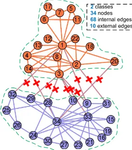
[image:2.576.94.231.471.626.2]In 2015, distance dynamics model has been proposed as a new community detection model of complex network [18]. It divides all edges into two categories: internal edge located in same community, and external edge crossed two differ-ent communities. By removing all external edges, distance dynamics model can naturally find the community structure of network. As shown in Figure 1, a simple social network is listed, containing 2 classes, 34 nodes, 68 internal edges and 10 external edges (red cross-marked line). To detect the community structure, the key is to remove the 10 external edges. Thus, distance dynamics model introduces interaction process to simulate the distance of each edge, and label the final type (internal edge or external edge) of each edge based on the distance. The interaction process can be described as follows: firstly, each edge is associated to an initial distance; then all edges interplay with its neighbors, the distance of each edge will shrink or expand gradually as time evolves. The nodes with highest similarity will synchronize first, the distance between them will decrease to 0 gradually. Mean-while, the nodes with high dissimilarity will become far away from each other, the distance between them will increase to 1 gradually; finally, the edge distance converges, if the edge distance equals to 1, the edge will be considered as external edge, otherwise, is the internal edge. The more details will be described in section II.A. Moreover, the distance dynamics model has some attractive features, such as ‘‘small commu-nity finding’’, ‘‘outlier discovery’’, and ‘‘intuitive commucommu-nity detection’’.
FIGURE 1. Idea of distance dynamics model.
However, with the development of information technology, the scale of network data is growing fast, the traditional distance dynamics model usually takes long time consump-tion or even fails to work when handling large-scale network. Besides, for dynamic interaction process, slow convergence problem of edge distance usually occurs, which is another
reason for causing the long time computation. Based on above drawbacks, it urgently requires developing parallel and effective community detection algorithms. The motivation of this study is to design a fast community detection algorithm for large network based on the distance dynamics model and preserving high cluster quality. Therefore, a parallel commu-nity detection algorithm, called P-Attractor, is proposed to contribute several matters:
1) Graph partitioning method: A graph partitioning method is proposed to divide large network into lots of sub-networks, yet maintaining the complete neigh-bor structure of the original network. The graph par-titioning method guarantees the feasibility of parallel dynamic interaction process.
2) A novel improved dynamic interaction model: The tra-ditional distance dynamics model has been improved to simulate the distance evolution. The update model is proposed to speed up the distance dynamics process, comparing with native Attractor model, the improved model could reduce 10% (average) computation time. 3) Slow-convergence problem scheme: Convergence
threshold and pre-judgment coefficient are designed for solving the slow-convergence problem, which help to accurately pre-judge the final distance of slow-converged edge and reduce interaction time steps. 4) Large-scale network community detection: Our
pro-posed approach contributes to handle community discovering problem for large-scale network within acceptable computation time. The execution time on 4 threads and 32 threads are around 10 hours and 2 hours, respectively. Our proposed algorithm is poten-tial to discover community from billion scale network, such as Uk-2007.
The remainder of the paper is organized as follows. The traditional distance dynamics model is described in section II. In section III and section IV we respectively analyze the graph partitioning, parallel dynamic interaction phase. In sectionV we show community detection phase and summarize the whole parallel community detection algorithm (P-Attractor). The results from our extensive experimental evaluations will present in the sectionVI. SectionVIIfinally concludes this paper.
II. BACKGROUND
A. TRADITIONAL DISTANCE DYNAMICS
In order to describe our algorithm more clearly, we introduce the background and interaction patterns firstly. Given an undirected graphG =(V,E,W),N(u) is a node set which consists of nodeu and his connected nodes, is defined as follows:
N(u)= {v∈V| {u,v} ∈E} ∪ {u}. (1) The Jaccard distance between nodeuand nodevis defined as:
d(u,v)=1−|N(u)∩N(v)|
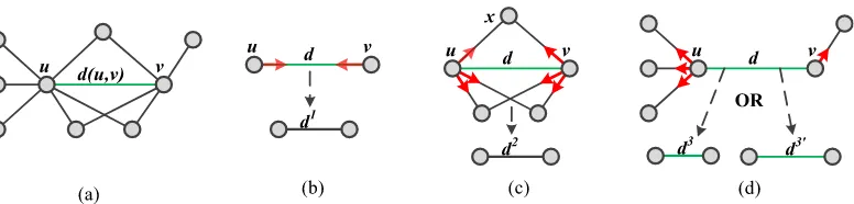
FIGURE 2. Three distinct interaction patterns. (a) Graph. (b)Influence from direct linked nodes. (c) Influence from common neighbors. (d) Influence from exclusive neighbors.
In the above equation, | ∗ | indicates the node number of set∗. The distance measures the similarity of the neighbor set between nodeuand nodev. For weighted undirected graph, due to the different weight of each edge, the Jaccard Distance changes, then the model is further extended as:
d(u,v)=1−
P
x∈N(u)∩N(v)(w(u,x)+w(v,x))
P
{x,y}∈E;x,y∈N(u)∪N(v)w(x,y)
. (3)
The traditional distance dynamics model consists of three interaction patterns, as shown in Figure 2.
1) PATTERNDI
Influence from direct linked nodes. The distance d(u,v) between nodeuand nodevare obviously influenced by two direct linked nodes u and v. Through mutual interactions, one node attracts another to move towards itself, and leads to decrease of the distanced(u,v) (Figure 2 (b)).DIis defined to indicate the influence between two direct linked nodes, as follows:
DI = −
f (1−d(u,v))
deg(u) +
f (1−d(u,v)) deg(v)
. (4) In pattern DI,deg(u) indicates the degree of node u, f (·)
is a coupling function, default is function sin(·). The term 1−d(u,v) implies the similarity of instinct structure or prop-erties between nodeuandv. The term 1/deg(u) is a normal-ized factor, which represents the different influences between linked nodes.
2) PATTERNCI
Influence from common neighbors. The distance d(u,v) is influenced by the common neighbor CN = (N(u)−u)∩
(N(v)−v)of nodeuandv, where the common neighbor is a node both connecting to nodeuandv. Due to each common neighbor will communicate with both nodeuandv, common neighbor will attract two end nodes to close itself, and leads to the decrease of the distanced(u,v) (Figure 2 (c)). The second interaction pattern is calledCI, is defined as follows:
CI(u)= 1
deg(u)·f (1−d(x,u))·(1−d(x,v)) CI(v)= 1
deg(v)·f (1−d(x,v))·(1−d(x,u)) CI = − X
x∈CN
(CI(u)+CI(v)).
(5)
In the pattern CI, for each common neighbor x, the two terms (1−d(x,u)) and (1−d(x,v)) are introduced to fur-ther measure the different influence between patternDI and patternCI.
3) PATTERNEI
Influence from exclusive neighbors. The influence from exclusive neighbor is seen as the third interaction pattern, where the distance d(u,v) will be influenced by exclusive neighborEN(u) = N(u)−(N(u)∩N(v)) or EN(v) = N(v)−(N(u)∩N(v)). The exclusive neighbor only con-nects to either nodeu or v (Figure 2 (d)). Each exclusive neighbor node form an external neighbor pair with the uncon-nected end node. In the dynamic interaction process, each exclusive neighbor will attract only one node (nodeuor v) to move towards itself. However, it’s hard to know whether another node will close to the exclusive neighbor or not. In order to clarify the positive or negative influence from exclusive neighbor, a cohesion parameter is introduced to measure the similarity of two nodes in exclusive neighbor pair, is defined as:
ρ (x,u)=
(
(1−d(x,v)), if (1−d(x,v))≥λ
(1−d(x,v))−λ, otherwise. (6) In the above equation,ρ(x,u) indicates the positive or nega-tive influence from the exclusive neighborsEN(u) to nodev. Based on the cohesion parameter, the third interaction pattern EIis defined as:
EI(u)= 1
deg(u)·f (1−d(x,u))·ρ (x,u) EI(v)= 1
deg(v)·f (1−d(y,v))·ρ (y,v) EI = −
X
x∈EN(u)
EI(u)+ X x∈EN(u)
EI(v)
.
(7)
Finally, the dynamics of distance d(u, v) between nodes uandvis governed by:
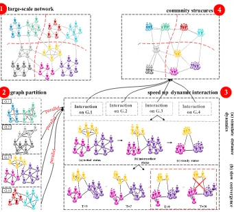
FIGURE 3. Illustration of parallel community detection based on distance dynamics.
B. PARALLEL DISTANCE DYNAMICS IDEAS
To give the basic idea of our algorithm, we take Figure 3 as an example, a large-scale artificial social network is listed, containing 9 groups represented by cartoon people of differ-ent colors. In order to quickly find the 9 groups, we adopt the ‘‘divide-and-conquer’’ strategy. Firstly, the original large net-work is divided into 4 sub-netnet-works (G.1, G.2, G.3, and G.4), each node of sub network keeps same neighbor structure with the original network, please see the Figure 3.2. After graph partitioning, we conduct dynamic interaction process on each sub-network in parallel mode. We suppose the interaction process is to discover opinion disparities among persons. We take G.3 as an example. At the beginning (initial status), every person usually has their own idea, the disparities of opinion (distances) with his neighbors are different, as shown in the Figure 3.3. Due to the influence from his/her known persons, the disparities of opinions (distance) among these persons gradually changes (increase or decrease) as time goes by, and reach immediate status. The immediate status usually goes through lots of time steps, such as fromT =1 to T = 16. In which, opinions of most persons converge quickly and only a few persons are irresolute. That’s a long time consumption to converge the opinions of these persons, such as from T = 9 to T = 16, we call this case as the slow-convergence. In order to solve the slow-convergence problem, we address pre-judgment strategy and obtain the
final distance whenT = 9, then we can save 7 time steps fromT = 10 to T = 16. Finally, we collect all external edges crossed multiple communities from all sub-networks, and find the community structure of original network by removing all external edges. The traditional distance dynam-ics model consists of three interaction patterns, as shown in Figure 2.
III. GRAPH PARTITIONING
To speed up the distance dynamics model, we partition large-scale network into many sub-networks (divide) and clustering each sub-network separately (conquer) and merge the cluster-ing results from all sub-networks. In this section, we present the graph partitioning phase.
A. ANALYSIS
Unlike other scalable community detection algorithms which based on drawing a sample or summarizing from network data, our method handles large-scale network by randomly partitioning networks into thousands of sub-networks with fixed size. However, the crucial question arises: Why does the partitioning technique works for our scalable community detection algorithm and what is the reason behind this?
community dynamically move together. Therefore, the local structure within each partition can be maintained. Thus, although the size of sub-network is smaller than the original large-scale network, the local structure of each sub-network node is still maintained and represented. That ensures correct-ness of detection results for each partition. In addition, dis-tance dynamics model is robust on noise and outlier objects. Thus, global outliers in the original large-scale can be easily identified in each separate partition. In summary, the ‘‘divide-and-conquer’’ strategy fits well to distance dynamics model, the distance dynamics model can effectively find the commu-nity structure of large-scale network in parallel mode, without relying on a powerful hardware environment. Moreover, there are several issues to concern: neighbor structure maintenance, edge equally partition and cross edge calculation.
1) NEIGHBOR STRUCTURE MAINTENANCE
In the distance dynamic model, the interaction scope of each node is only affected by its neighbors, so the distance dynamic model will still work well if each node’s neighbor structure can be complete guaranteed. This feature prompts us to adopt the ‘‘divide and conquer’’ concept to optimize the calculation time of distance dynamic models in large-scale networks. Thus, we divide the large-large-scale network into multiple small-scale sub-networks and independently use dis-tance dynamic model for each sub-network, which helps to improve the computational efficiency. However, in order to accurately discover the community structure of the original large-scale network based on the calculation results of all the sub-networks, we should maintain the neighbor structure of each node. After the network has been divided, the topology of each node in the sub-network will not completely be consistent with the original network, especially the marginal edges, some of its neighbors may be located in other networks. Therefore, we need to ensure each node of the sub-network to keep same neighbor structure as far as possible.
2) EDGE EQUALLY PARTITION
After graph partitioning, all sub-networks will parallel exe-cute the distance dynamics model for calculating the final distance of each edge. In order to minimize the computation time, we should evenly partition the edges to guarantee each sub-network has the same edge number. Because the distance
dynamics model is an edge-oriented dynamic community detection model, so there is a positive correlation between edge number and time computation.
3) CROSS EDGE CALCULATION
Through graph partitioning, all edges of each sub-network will be naturally classified into two categories: inner edge and cross edge. For each inner edge, two endpoints belong to same sub-network. On the contrary, for each cross edge, two endpoints belong to different sub-networks. Here, each inner edge keeps same neighbor structure with the original network, while, cross edges may differ. Therefore, in order to get the accurate final distance of each cross edge, we intro-duce edge-circle as a complementary structure to maintain the complete neighbors of each cross edge.
B. CIRCLE DEFINITIONS
For graph partitioning, node migration and edge migration are very important process. Node migration aims to maintain the neighbor structure of each node, and keep the same edge number for each sub-network. The goal of edge migration is to supplement lost neighbors of cross edge. In order to migrate nodes or cross edges more accurately, node-circle and edge-circle are defined.
Definition 1 (Node-Circle): Given a social network (Figure 4(a)), node-circle means the social circle of a node, and the active scope of a node, please see Figure 4(b). The node-circle consists of this node, his neighbors and all edges between them, and defined as follows:
NC(u)=(CV,CE), (9) where, CV = {x|x∈N(u)} and CE = {(x,y)|x,y∈CV}. In this paper, we consider that a node should stay with its node-circle. When its node-circle belongs to a sub-network, the node should not be migrated. Otherwise, a node crosses multiple sub-networks, it should migrate to the sub-network having most nodes of the node-circle. Moreover, by matching the node number and the range of the sub-network node, we can quickly discover target sub-network that need to be migrated. To supplement the lost neighbor structure of cross edge, we define the edge-circle in this paper.
[image:5.576.88.491.612.710.2]Definition 2 (Edge-Circle): Given a social network (Figure 4(a)), edge-circle represents the social circle of each
edge, and the active range of a node, please see figure 4(c). The edge-circle consists of two end nodes, its neighbor set of two end nodes and all edges between them, is defined as follows:
EC(e(u,v))=(EV,EE), (10) where,EV =x|x ∈N(u)∪N(v), andEE =(x,y)|x,y∈ EV. We also consider that a cross edge should stay with its edge-circle. When edge-circle of one edge belongs to one sub-network, if the edge is an inner edge, then it should not be migrated. When edge-circle of one edge belongs to multiple sub-networks and the edge is a cross edge, then it needs to be migrated to the sub-network having most nodes of the edge-circle. We have two goals on cross edge migration. On one hand, it helps each cross edge to stay with the most right sub-network, which has most neighbors of this edge, on the other hand, at cross edge migration phase, it also helps to fill the lost neighbors based on edge-circle, and keep the complete neighbor structure of each cross edge.
C. PARTITIONING PROCESS
In summary, the whole process of graph partitioning consists of three steps:
Step 1, parallel initial partition. According to the node number, we generate multiple sequential sub-networks, ensure that the number of nodes in each sub-network is the same and the node number is continuous. By matching minimum end node of each edge with the node range of sub-network, we parallel divide all edges into sub-networks as initial partition. For example, a social network hasNNnodes andTT edges, we need to divide the network intoSN sub-networks. Firstly, we generate the node scope of SN sub-networks, where the node of first sub-network ranges from 0 to NN/SN, the second ranges from NN/SN +1 to 2∗ NN/SN, and so on. Secondly, we OpenSN processes to read edges in parallel, the first process reads from 1 to the edge of TT/SN, the second process thread reads from TT/SN +1 to 2 ∗ TT/SN, and so on. For each edge, corresponding process calculates the serial number of minimum end node, then assigns each edge to the sub-network until all edges are finished.
Step 2, parallel node migration. After initial partition, we start to migrate node from sub-networks in parallel mode. For one sub-network, we traverse each node, and calculate its node-circle. When node’s node-circle belongs to the current sub-network, then the node remains, and go to next node. When a node and its node-circle belongs to different sub-network, then calculate the target sub-network having most nodes of node-circle, and migrate the node and all directly linked edges to the target sub-network. When all nodes have been completed, the node migration process is ended.
Step 3, parallel cross edge migration. After node migra-tion, each cross edge’s neighbor structure is uncompleted. We start cross edge migration for sub-networks in parallel mode. For one sub-network, traverse each cross edge, cal-culate the edge-circle and the target sub-network with most nodes of edge-circle. When the target sub-network is current sub-network, insert the edge-circle into current sub-network as the supplementary neighbor structure of cross edge, go to next cross edge. When the target sub-network is not cur-rent network, migrate the cross edge to the target sub-network, insert the edge-circle into the target sub-network as the supplementary neighbor structure of the cross edge, go to next cross edge. When all cross edges have been completed, the cross edge migration is over.
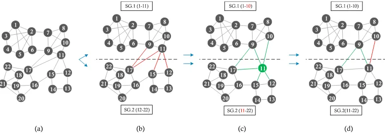
[image:6.576.92.483.568.705.2]To illustrate graph partitioning more clearly, let’s take Figure 5 as an example, a large-scale network contains 22 nodes (black points) and 41 edges (black solid lines between points), shown as Figure 5 (a). In the initial phase (Figure 5 (b)), the nodes from 1 to 11 and corresponding edges are auto assigned to first sub-network SG.1. Mean-while, the nodes from 12 to 22 and corresponding edges are assigned to second sub-network SG.2. Here, three cross edges (red solid lines) are allocated to first sub-network, because the minimum end node of three edges belong to first sub-network. After initial partitioning, the number of edges in two sub-networks is uneven, the edges of SG.1 are more than the edges of SG.2. In the second phase (Figure 5 (c)), we start node migration to maintain neighbor structure and keep edge even partition. Here, node 11 (green circle) and correspond-ing edges (green edges) are migrated from SG.1 to SG.2. After node migration, 3 cross edges don’t have complete
FIGURE 6. Illustration of slow-convergence.
neighbors. In the third phase (Figure 5 (d)), we start cross edge migration to supplement the lost neighbor structure of each cross. Based on the edge-circle, edge e(10, 11) is migrated from SG.2 to SG.1, and the edge-circle of 3 cross edges are inserted to SG.1 or SG.2. After graph partitioning, SG.1 has 21 edges and SG.2 has 22 edges.
IV. PARALLEL DYNAMIC INTERACTION
In this section, firstly, we describe the slow-convergence problem and corresponding pre-judgment optimization strat-egy. Then, we improve the distance dynamics model and address the pre-judgment strategy. Finally, by using the improved distance dynamics model, we parallel execute the interaction process for all sub-networks.
A. SLOW-CONVERGENCE PROBLEM
In traditional distance dynamics model, slow-convergence problem usually cause our concern on unnecessary time con-sumption. In the distance dynamic model, a dynamic interac-tion process is introduced to simulate the dynamics of each distance. Before all the distances converge (the steady state), the entire interaction process needs to go through multiple time steps. Most of the distances have converged within the first 3-8 time steps, and only a very small distance needs long time to reach the steady state. That is, in order to com-plete the convergence of all distances, most distances have to wait a long process after they have converged. In some special networks, we may even encounter non-convergence situations. The distances of some edges increase or decrease go and back, and the final state will never reach.
In the Figure 6, a social network contains two communi-ties represented by different color, and we use the distance dynamics model to find its community structure. After going through 30 iterations, all distances converge whenT =30. However, throughout the interaction process, 17 distances converge beforeT =10. In order to converge the 2 remain-ing distances d(12,6) and d(5,4), we need to take more 20 time steps. Therefore, we call this situation as the slow-convergence. In addition, it is not difficult to find that, no mat-ter what the final status of 2 distances are, the detected community structure is unchanged.
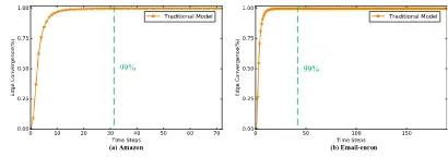
In order to further prove the existence of slow-convergence, two real world networks are selected to execute the distance dynamics model. Going through many repeated experiments, Figure 7 shows the existence of slow-convergence. In the
[image:7.576.313.518.260.332.2]Figure 7, the green dashed line means the time steps when 99% distances are converged. It is obviously that the slow-convergence problem seriously influences the computation time of the distance dynamics model.
FIGURE 7. Slow-convergence of different networks.
To solve the slow-convergence problem, it is key to accu-rately pre-judge the final distance of slow-converged edge. For distance dynamics model, each edge is only influenced by its neighbor, so we address the edge-circle to pre-judge the final status of slow-converged edge. For a slow-converged edgee(u,v), all edgesEEof edge-circleEC(e) are classified into two categories: public neighbor edge and private neigh-bor edge. Public neighneigh-bor edge PubE(e) = NC(u) .E ∩ NC(v)connects the neighbor set of two end nodes at the same time. In the process of dynamic interaction, public neighbors will attract two end nodes ofe(u,v) to move together, and the distance ofe(u,v) will decrease. As opposed to public neigh-bor edge, each private neighneigh-bor edgePriE(e)=(NC(u) .E∪ NC(v) .E)−PubE(e)only connects the neighbor set of one end node ofe(u,v). So, it will prevent two end nodes ofe(u,v) to move together, and the distance ofe(u,v) will increase.
To further enhance the accuracy of pre-judgment, we also consider the converged status of neighbor edge. Therefore, we design three rules to pre-judge the final distance of slow-converged edge.
(1) When the final distance of one converged public neigh-bor edge in the edge-circle equals to 1, then we think the final distance of slow-converged edge should be 1. Because the converged public neighbor edge has been implied two end nodes of the slow-converged edge may belong to different communities.
(3) When previous two rules are not satisfied, we use the edge-circle to determine the final distance value. When the number of public neighbor edge is more than the number of private neighbor edge, the final distance of slow-converged edge should be 0. On the contrary, we think the final distance should be 1.
In this paper, we merge above three rules, and propose a pre-judgment coefficient to determine the final distance of slow-converged edge. The pre-judgment coefficient is defined as follows:
PreC =
1, ∃e(x,y)∈PubEd(x,y)=1
0, ∀e(x,y)∈PubEd(x,y)=0 1,
|PriE(e(u,v))|
|EC(e(u,v)) .E|
>0.5
0,
|PriE(e(u,v))|
|EC(e(u,v)) .E|
≤0.5,
(11)
whereEC(e) is the edge-circle ofe(u,v), thePriE(e) is the private neighbor edge, the PubE(e) is the public neighbor edge. The effectiveness of pre-judgment coefficient will be proved in the sectionVI.D.
B. IMPROVED DISTANCE DYNAMICS MODEL
In order to handle slow-converged problem, convergence thresholdτ is addressed as a switch to determine the timing of pre-judgment process start, and calculate the final distance of slow-converged edge. It’s defined as follows:
CF =
1, |CE|
|E| ≥τ
0, |CE|
|E| < τ,
(12)
where, the term| ∗ |indicates the number of set∗, andCE as the converged edge set. When the percentage of converged edges exceeds convergence threshold value, the pre-judgment coefficient start the pre-judgment process. So we improve distance dynamics model and formulate distance dynamics of each edge as follows:
d(u,v,t+1)=(1−CF(t))·EI
+CF(t)·PreC(u,v,t) , (13) where,d(u,v,t+1)is the renewed distance of edgee(u,v) at time stept+1, andEI =d(u,v,t)+DI(t)+CI(t)+ EI(t) .CF(t) is the pre-judgment switch function, and deter-mines the timing of pre-judgment process. When theCF(t) is 0, the three interaction patterns start to influence the distance d(u,v), whereDI(t),CI(t) andEI(t) are three different influ-ences respectively from the directed node, common neigh-bors, and exclusive neighbors at time stept. When theCF(t) is 1, we start the pre-judgment process, use the pre-judgment coefficient to determine the final distance of slow-converged edgee(u,v).
C. PARALLEL INTERACTION PROCESS
Based on the improved distance dynamics model, all sub-networks will parallel execute the dynamic interaction pro-cess to simulate the dynamics of each distance. For a sub-network, the process of dynamic interaction is as follows:
Step 1, at initial time (t =0), no interaction process, each edge in the sub-network (including the edge-circle of cross edge) is associated with an initial distance. Here, the initial value is computed according to the Jaccord distance with Definition 2 or Definition 3.
Step 2, as time evolves, we start the dynamic
interac-tion. When the percentage of converged distances is less than the convergence thresholdτ (CF = 0), we use three dynamic interaction patterns (Eq. (4), Eq. (5) and Eq. (7)) to simulate the dynamics of each distance. Driven by the neighbor structure, each distance will decrease or increase gradually. The nodes with the highest similarity will syn-chronize first, the distance between them will decrease to 0. Meanwhile, the nodes with the highest dissimilarity will be far away, the distance between them will increase to 1. Going through a sequential process, more and more nodes will synchronize, and distances will converge.
Step 3, when the percentage of converged distances
exceeds convergence threshold (CF = 1), we start pre-judgment process for slow-converged edge. By calculating the pre-judgment coefficient (Eq. (11)), each slow-converged edge will obtain final distance value.
Step 4, finally, all distances in the sub-network will con-verge, and the edges with long distances (i.e.d(u,v)=1) are collected.
To describe above process more clearly, Figure 8 shows the process of dynamic interaction. Four statuses of network are listed in the Figure 8 (a)-(d) fromt = 0 tot = 12. Figure 8 (a) shows the initial status of network (t=0), where each edge has an initial distance. Figure 8 (b) shows the first immediate status (t = 1), where each distance changes by as time involves. Figure 8 (c) shows the slow-convergence status (t = 11), where only three distances (red solid lines) don’t converge. Then, we start the pre-judgment process for the slow-converged edge. When (t =12), the steady status is coming, all distances converge (either 0 or 1), and all edges with long distances are collected to prepare for community detection of original large network.
D. PARAMETER DISCUSSION
FIGURE 8. Illustration of dynamic interaction. (a) the initial status; (b) the immediate status after one time step; (c) the slow-convergence status; (d) the final status.
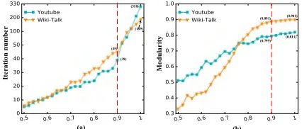
(ranging from 0 to 1), the iteration number and modularity value keep changing. In the Figure 9 (a), we observe the dynamic change of iteration number. When the convergence thresholdτ exceeds 0.8, with minor change of convergence thresholdτ, the iteration number rapidly increases. For exam-ple, when τ ranges from 0.8 to 1, the iteration number in Youtube network ranges from 24 to 318. Meanwhile, the iter-ation number in Wiki-Talk network ranges from 33 to 189. In the Figure 9 (b), we observe the dynamic change of mod-ularityQ. Generally, the larger the modularityQis, the better cluster accuracy will be. When the convergence thresholdτ is less than 0.85, with minor change ofτ, the modularityQ greatly increases and the cluster accuracy rapidly improves. In summary, 0.9 is selected as the recommended convergence threshold in following experiments. Because, when the con-vergence threshold is 0.9, the iteration number (Youtube is 39 and Wiki-Talk is 45) is far less than the value of complete iteration (Youtube is 318 and Wiki-Talk is 189, respectively). Similarly, the cluster accuracy (modularity Q, Youtube is 0.80 and Wiki-Talk is 0.89) is close to the cluster accuracy of complete iteration (Youtube is 0.81 and Wiki-Talk is 0.90, respectively).
V. P-ATTRACTOR: PARALLEL COMMUNITY DETECTION BASED ON DISTANCE DYNAMICS
A. P-ATTRACTOR ALGORITHM
In summary, the whole community detection process can be simply summarized as three phases:
Phase 1, graph partitioning (divide). According to the node number, we generate multiple sequential sub-networks, each sub-network has the same number of nodes. By matching minimum end node of each edge with the node range of
FIGURE 9. Sensitivity of convergence thresholdτ.
sub-network, we parallel divide all edges of large network into sub-networks as initial partition. After initial partition, we start node migration in parallel mode to maintain the neighbor structure of each node, and keep edge even parti-tion. After node migration, we start cross edge migration to supplement the lost neighbors of cross edge.
Phase 2, parallel dynamic interaction (conquer). Using
the improved distance dynamics model, all sub-networks parallel execute dynamic interaction process to get the final distance of each edge. In the dynamic interaction process of sub-network, each edge is associated with an initial dis-tance; as time evolves, each distance would expand or shrink gradually by the influence from three interaction patterns; when the percentage of converged distances is more than the convergence thresholdτ, the pre-judgment process of slow-converged edge is started, pre-judgment coefficient is used to determine the final distance of slow-converged edge; finally, all distances will converge (either 0 or 1), and the edges with long distance will be collected (the distance value is 1) to prepare for the next phase.
Phase 3, community detection. All edges with long
dis-tance in the sub-networks are merged to form the external edge set of large-scale network. Using the idea of distance dynamic model, we remove all external edges, cut off the connection between communities, and find the community structure of large network quickly.
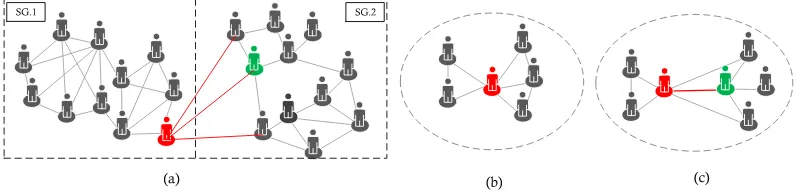
We take Figure 10 as an example to illustrate the com-munity detection process. By using the graph partitioning, the large-scale network has been divided into two sub-networks (SG.1 and SG.2). After graph partitioning, we start the parallel dynamic interaction on the sub-networks to com-pute the final distance of each edge. After parallel dynamic interaction, each sub-network produces long edge set LD (SG.1.LD and SG.2.LD), where the distance of each edge equals to 1. We merge two long edge set as the external edge set of original large network. By removing all external edges (red or purple edges), the community structure of large-scale network can be naturally detected.
B. TIME COMPLEXITY
[image:9.576.50.263.620.711.2]FIGURE 10. Process of community detection.
edges in original large-scale network andSN is the number of networks. At the second phase, due to each sub-network parallel execute the distance dynamics model, so the time complexity comes from the dynamic interaction. In the dynamic interaction, the initial distance of each edge can be computed in graph partitioning phase, so the time complexity is(T ·k·(|E|/SN))wherekis the average number of neigh-bors andTis the time steps. At the third phase, all long edges could be removed in the second phase, so the time consump-tion can be ignored. In summary, the time complexity of our algorithm isO (|E|/SN)2+T·k·(|E|/SN)
.
VI. EXPERIMENTS
In this section, we present experimental evaluation of P-Attractor algorithm on several real world networks as well as artificial networks.
A. EXPERIMENTAL SETUP
In order to simulate the large-scale network, we take a high-performance server which configures 2× Intel Xeon E5-2600 series processors and 176GB of memory. Each pro-cessor has 16 cores, and able to concurrently run 32 threads for multithreaded applications in maximum. Besides, each processor has a L3 cache of 20 MB at a frequency of 3.3 GHz, with two 8 GT/s QuickPath Interconnect (QPI) links between processors. In addition, our algorithm is written in python, and parallel executed in multiple-thread mode.
We perform experiments on a variety of networks, as listed in Table 1. We focus on real world networks, and some syn-thetic instances are included as well. The real world networks include a web graph (Uk-2007), a road network (RoadNet-PA), four social networks (Wiki-Talk, Youtube, Orkut, LiveJournal). Among the real world networks, Youtube, Orkut, and LiveJournal are three ground-truth networks. Two synthetic networks (LFR1 and LFR2) are generated with the community ground-truth by using the LFR benchmark [22], whereuis the mixing parameter andkis the average degree of each node
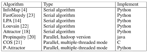
[image:10.576.296.538.82.243.2]We select several community detection algorithms in the state-of-the-art to compare with our algorithm, as shown
TABLE 1.Networks.
in table 2. In which, InfoMap, FastGreedy and Louvain are considered as being widely used algorithms for dis-joint community detection, the LPA algorithm shows linear time complexity, we can download the implementations of Python version from open source website. In addition, two standard parallel algorithms Propinquity (the source code are available at: http://dbgroup.cs.tsinghua.edu.cn/zhangyz/ kdd09/) and COS (the source code are available at: https:// sourceforge.net/p/cosparallel/wiki/SetupAndCompile/) are also addressed to be compared with, where, Propinquity addressed BSP parallel model. Also, Attractor algorithm as the native algorithm based on the traditional distance dynamics model is indispensable.
TABLE 2.Comparison Algorithms.
[image:10.576.297.537.456.542.2]as the rate of correctly number of identifying nodes among the total node number of network in the community. The CDA is defined as follows:
CDA= k
P
i=1
maxnCi∩Cjnew|Cjnew∈Cnew
o
n , (14)
where, j = 1,2,· · ·,l, C is original community set and can be expressed as C = {C1,C2,· · · ,CK}, Cnew is the
detected community set,Cnew = C1new,C2new,· · · ,Clnew , and maxnCi∩Cjnew|Cjnew∈Cnew
o
represents the max com-mon node number of all community set and thei−th com-munity,n is the node number of network. The higher CDA value means better detection accuracy and quality.
B. COMMUNITY DETECTION ANALYSIS
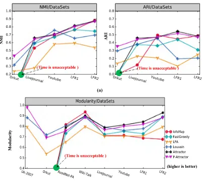
[image:11.576.304.529.129.250.2]The first objective of experimental evaluation is to test the cluster quality of our algorithm, and observe the differ-ence between our P-Attractor algorithm and native Attrac-tor algorithm. We repeatedly test 6 different algorithms on 8 networks, and select the best results to compare, where P-Attractor algorithm is executed on four threads. The NMI and ARI metrics are used to measure the cluster quality for the ground-truth networks (Orkut, LiveJournal, Youtube, LFR1, LFR2), and the Modularity metrics is used to measure the cluster quality.
FIGURE 11. Cluster quality on different networks.
Figure 11 shows the cluster quality of 6 algorithms on different networks, Figure 11 (a) shows the NMI and ARI comparison, and Figure 11(b) shows the modularity com-parison. As we can see from Figure 11, four algorithms (P-Attractor, Attractor, InfoMap, and Louvain) show better performance (NMI, ARI, and Modularity) than other two algorithms (LPA and FastGreedy ). Our P-Attractor algorithm presents almost the same cluster quality with the Attractor algorithm. However, when the number of edges exceeds over one hundred million (large-scale), then the computation time
of Attractor, InfoMap, and FastGreedy become unacceptable, please see the big greed points in the Figure 11. For the large-scale networks (Orkut, Uk-2007, LiveJournal), P-Attractor on 4 threads works well and shows good cluster quality.
FIGURE 12. Detected community structure on LFR1.
Figure 12 shows the detected community structure between 5 traditional serial algorithms and P-Attractor on LFR1. Because the LFR1 contains 2 million edges and 116 commu-nities, in order to illustrate the detected communities more clearly, we sample 4 communities and 2372 nodes from LFR1. Figure 12 (a) is the ground-truth of LFR1, the sub-network in the grey circle is the community structure of sampling 2372 nodes. Figure 12 (b) shows the detected com-munities of Attractor, and the number of detected commu-nity is 5 at the 2372 sampling nodes. Figure 12 (c) shows the detected communities of P-Attractor, the number of the detected community is also 5. We observe that, Attrac-tor (5 communities), P-AttracAttrac-tor (5 communities), InfoMap (3 communities), and LPA (5 communities) show better per-formance than other two algorithms (Louvain (6 communi-ties), FastGreedy (6 communities)) on LFR1 network.
Table 3 shows the computation time of 5 traditional serial algorithms and P-Attractor on 8 different networks. Among the five algorithms (InfoMap, FastGreedy, LPA, Louvain, and Attractor), LPA algorithm shows the fastest speed, Lou-vain and InfoMap algorithms are the next, FastGreedy and Attractor algorithms are the worst. Focusing on the Attractor algorithm, with the increase of network scale, the increased computation time on Attractor is obviously fast than other four algorithms. When the number of edge exceeds over one hundred million (Uk-2007 and Orkut), the computation time of Attractor algorithm is unacceptable. However, our P-Attractor algorithm gets a reasonable computation time by using parallel execution with 4 threads. On the Uk-2007 net-work, P-Attractor algorithm takes 34599 seconds, and finds the community structure form 3.3 billion edges. For the Orkut network, P-Attractor algorithm takes 1582 seconds, and finds the community structure from 100 million edges. That is, P-Attractor shows the ability to speed up the distance dynam-ics model for large network, yet guaranteeing good cluster quality.
[image:11.576.57.257.394.579.2]TABLE 3. Time (s).
from table 3, when the network scale is large, such as over 10 million level network, due to the limit of machine hard-ware and high time complexity, single serial algorithm may fail to detect the community structure. Propinquity and COS as two standard parallel algorithm, we conduct two groups of experiments to analyze the comparison of parallel algorithms. Firstly, we run three algorithms on three ground-truth datasets and one synthetic datasets. Figure 13(a) shows the computation time of our P-Attractor and the two parallel algorithms, the number on the bar represents CDA score. We can see that, all three algorithms perform good execution time on youtube dataset and good CDA score caused by its clear community structure, all the three algorithm show good CDA result on LFR2, which means high community detection accuracy of algorithm, LiveJournal and youbute is the second, Orkut is the worst because of its uneven edge dis-tribution. On million scale network, Convergence threshold and pre-judgment coefficient contribute to solve the slow-convergence problem, so the parallel computation becomes remarkable when network scale increases beyond the capa-bility of a single-serial algorithm which were compared on previous experiments. Although the run time of P-Attractor is better than other two parallel algorithm, indicating the par-allel interaction process model fit the large-scale networks, but COS shows better CDA score on some networks, such as low density network like youtube and LFR2. Propinquity shows worst CDA score in average, the low CDA results may be caused by its average vertex degree calculation method, which equals toE|/|V|, that is not meet the actual network situation in real world, although it can highly reduce its time complexity.
[image:12.576.37.278.84.183.2]Then, we try to test the speeded-up performance on bil-lion scale dataset of proposed parallel algorithms. As shown in Figure 13(b), by comparing execution time of Propinquity, COS and P-Attractor on Uk-2007, we use four configurations for three algorithm, respectively, run on 8,12,18,24 threads, each experiment runs three times and takes the average time. As we can see, with the increase of its parallelism degree, all three algorithm show speed up capability, under same configuration of parallel threads, P-Attractor performs better execution time, when the complexity of network relations over 100 million degree, the advantages of parallel algo-rithms become significant, which also confirm that our par-allel community detection method has excellent scalability.
FIGURE 13. Comparison of parallel algorithms.
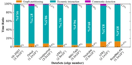
[image:12.576.310.525.407.513.2]Propinquity takes up most of the time on initialization of task allocation and data transfer between nodes, while it contains more file operations in Hadoop’s iterative process, and its proportion of the initial time is not negligible, with parallel machine increases, Propinquity traps into ‘‘long tail’’ phe-nomenon, resulting higher computation time than the other two algorithms. We can conclude that, our proposed method has strong practicability when handling with large networks. The details of parallel scalability analysis will be discussed on later section VI.E. Moreover, we further analyze the time proportion of different phases in P-Attractor, as shown in Figure 14. The time proportion of dynamic interaction con-sumes more than 85%. The proportion of graph partitioning is less than 14%, and the proportion of community detection is less than 2%. Besides, we can find that, with the increase of network scale, the time proportion of graph partitioning and community detection decreases gradually.
FIGURE 14. Computation time on different phases.
C. GRAPH PARTITIONING ANALYSIS
FIGURE 15. Performance analysis of graph partitioning.
FIGURE 16. Performance analysis of the improved distance dynamics model.
nodes in each sub-network is the same. However, the 8 dif-ferent networks have difdif-ferent densities and each node in the network has a different degree. As a result, the number of edges in each sub-network is different. The edge number of one of sub-graph exceeds the half edges in Wiki-Talk, LFR1, LFR2, Orkut, Uk-2007. (2) The node migration assures each sub-network has almost same number of edges, the number of edges in the sub-network is close to the average number (the green dashed line). (3) The cross edge migration further optimizes the graph partitioning, and decreases the difference of edge number among all sub-networks.
D. IMPROVED MODEL ANALYSIS
The third objective of the experiments is to compare the traditional distance dynamic model and the improved dis-tance dynamic model on three aspects, including interaction steps (time period), the Modularity, and the calculation time to verify the performance of the improved model. For the improved distance dynamics model, a convergence thresh-old τ is used as the threshold to determine the dynamic interaction process whether goes into the slow convergence, and a pre-judgment coefficient is used to pre-judge the final distance of slow-converged edge. Based on the analysis in
sectionIV.D, 0.9 is selected as the recommended value of convergence thresholdτ in this paper.
Figure 16 shows the performance comparison of the improved distance dynamics model and traditional distance dynamics model. As shown in the Figure 16(a), we com-pare the iteration number of two models. It’s obvious that the improved distance dynamics model greatly reduces the iteration number, and the iteration number of improved model is less than 50. In the Figure 16(b), the modularity value of improved model models shows almost same modularity value as the traditional model. It demonstrate the accuracy of pre-judgment process and the pre-judgment coefficient. In the Figure 16(c), we compare the computation time of two models. We find that, with the increase of edge, the com-putation time presents the linear growth. Moreover, compar-ing with the traditional model, our improved model reduces 10% (average) computation time. As the scale of the net-work increases, the time saved(red text) is also gradually increasing.
E. SCALABLE ANALYSIS
FIGURE 17. Computation time with different threads.
different number of parallel threads, we compare the compu-tation time and the relative speedup on 8 different networks.
[image:14.576.42.274.383.501.2]Figure 17 shows the computation time of P-Attractor algo-rithm on 8 different networks. As the number of threads increases, the computation time of P-Attractor decreases rapidly, and the downward trend is almost linear. We take the Uk-2007 as an example, the execution time on 4 threads is around 40000 seconds, but the execution time on 64 threads is only 4700 seconds. In additional, if the networks show different degree distribution, the speedup of computation time will be slightly different. Such as, the speed up on Roadnet-PA network is better than the Wiki-Talk network.
FIGURE 18. Relative speedup on 4 threads.
Figure 18 shows the relative speedup with 4 threads on different networks. Here, the black points are the relative speedup of different threads, and the red dashed line means the trend line of relative speedup. From the Figure 18, we can get the following observations. (1) As the number of threads increases, the relative speedup increases gradually. Such as, for the Uk-2007 network, the relative speed up is 4.7 x on 18 threads, the relative speed up increases to 7.9× on 32 threads. (2) Under the same number of thread, the relative speedup is slightly different for different networks. For exam-ple, under the 18 threads, the relative speedup of RoadNet-PA is 5.5×, the speedup of Wiki-Talk is 5.6×, the speedup of Youtube is 5.1×, the speedup of LFR1 is 4.4×, the speedup of Orkut is 4.8×, the speedup of Uk-2007 is 4.7×, the speedup of LiveJournal is 4.0×, and the speedup of LFR2 is 3.8×. (3) With the increase of threads, the increase degree of relative speedup decreases gradually. That is, the increase degree of
relative speedup on 18 threads is larger than the increase degree on 32 threads. It can be proved in the Figure 18, where the black point of 32 threads is under the increase trend line of relative speedup (red dash line) of 18 threads.
VII. CONCLUSIONS
Attractor algorithm may fail to discover community from billion large scale network within acceptable computation time. We propose P-Attractor algorithm and try to detect com-munity from the large scale network and solve the slow con-vergence problem. To improve the usability and efficiency of distance dynamics model on large-scale network community detection, P-Attractor, is proposed. We address the ‘‘divide-and-conquer’’ strategy to speed up the distance dynamics model. P-Attractor firstly divides the large-scale network into lots of sub-networks, then parallel cluster each sub-network to get the final distance of each edge by using the distance dynamics model, collects all edges with long distance from all sub-networks, and finally removes all edges with long distance for finding the community structure of large-scale network. Moreover, in order to solve the slow-convergence problem, we improve the distance dynamics model and intro-duce the pre-judgment of slow-converged edge. We conduct extensive experiments on multiple real-world and synthetic networks, the results demonstrate it can work well for large-scale network (Orkut) and very large-scale network (Uk-2007). Moreover, the cluster quality (NMI, ARI, and Modularity value, CDA score) of P-Attractor is close to the quality of Attractor. As the number of threads increases, the computation time of our P-Attractor algorithm could be further optimized. Otherwise, by addressing the conver-gence threshold, the computational time of improved distance dynamics model has been further enhanced.
In our future work, we plan to work on other parallel programming paradigms and compare their performance with our parallel approach. In addition, the P-Attractor mainly aims at detect community from static complex networks. In the future work, the community discovery algorithms of dynamic networks and high-order networks will be further studied.
ACKNOWLEDGMENT
The authors thank the experimental equipments provided by National Super Computing Center of Changsha. Also, they would like to thank those anonymous reviewers for their constructive suggestions.
REFERENCES
[1] S. Fortunato, ‘‘Community detection in graphs,’’Phys. Rep., vol. 486, nos. 3–5, pp. 75–174, 2010.
[2] A. Lancichinetti and S. Fortunato, ‘‘Community detection algorithms: A comparative analysis,’’Phys. Rev. E, Stat. Phys. Plasmas Fluids Relat. Interdiscip. Top., vol. 80, no. 5, p. 056117, 2009.
[4] M. Rosvall and C. T. Bergstrom, ‘‘Maps of random walks on complex net-works reveal community structure,’’Proc. Nat. Acad. Sci. USA, vol. 105, no. 2, pp. 1118–1123, 2008.
[5] Y. Li, K. He, D. Bindel, and J. E. Hopcroft, ‘‘Uncovering the small community structure in large networks: A local spectral approach,’’ in Proc. 24th Int. Conf. World Wide Web, 2015, pp. 658–668.
[6] B. W. Kernighan and S. Lin, ‘‘An efficient heuristic procedure for parti-tioning graphs,’’Bell Syst. Tech. J., vol. 49, no. 2, pp. 291–307, Feb. 1970. [7] M. E. J. Newman, ‘‘Spectral methods for community detection and graph partitioning,’’Phys. Rev. E, Stat. Phys. Plasmas Fluids Relat. Interdiscip. Top., vol. 88, no. 4, p. 042822, 2013.
[8] M. C. V. Nascimento, ‘‘Community detection in networks via a spec-tral heuristic based on the clustering coefficient,’’Discrete Appl. Math., vol. 176, pp. 89–99, Oct. 2014.
[9] M. E. J. Newman and M. Girvan, ‘‘Finding and evaluating community structure in networks,’’Phys. Rev. E, Stat. Phys. Plasmas Fluids Relat. Interdiscip. Top., vol. 69, p. 026113, Feb. 2004.
[10] R. Aktunc, I. H. Toroslu, M. Ozer, and H. Davulcu, ‘‘A dynamic modularity based community detection algorithm for large-scale networks: DSLM,’’ inProc. IEEE/ACM Int. Conf. Adv. Social Netw. Anal. Mining (ASONAM), Aug. 2015, pp. 1177–1183.
[11] J. Xianget al., ‘‘Local modularity for community detection in complex networks,’’Phys. A, Stat. Mech. Appl., vol. 443, pp. 451–459, Feb. 2016. [12] S. Fortunato and M. Barthélemy, ‘‘Resolution limit in community
detec-tion,’’Proc. Nat. Acad. Sci. USA, vol. 104, no. 1, pp. 36–41, 2007. [13] U. N. Raghavan, R. Albert, and S. Kumara, ‘‘Near linear time algorithm to
detect community structures in large-scale networks,’’Phys. Rev. E, Stat. Phys. Plasmas Fluids Relat. Interdiscip. Top., vol. 76, no. 3, p. 036106, 2007.
[14] P. Pons and M. Latapy, ‘‘Computing communities in large networks using random walks,’’ inProc. Int. Symp. Comput. Inf. Sci., 2005, pp. 284–293. [15] A. Arenas and A. Diaz-Guilera, ‘‘Synchronization and modularity in com-plex networks,’’Eur. Phys. J. Special Topics, vol. 143, no. 1, pp. 19–25, 2007.
[16] C. L. Staudt and H. Meyerhenke, ‘‘Engineering parallel algorithms for community detection in massive networks,’’IEEE Trans. Parallel Distrib. Syst., vol. 27, no. 1, pp. 171–184, Jan. 2016.
[17] H. Sun, J. Liu, J. Huang, G. Wang, X. Jia, and Q. Song, ‘‘LinkLPA: A link-based label propagation algorithm for overlapping community detection in networks,’’Comput. Intell., vol. 33, no. 2, pp. 308–331, 2017.
[18] J. Shao, Z. Han, Q. Yang, and T. Zhou, ‘‘Community detection based on distance dynamics,’’ inProc. 21th ACM SIGKDD Int. Conf. Knowl. Discovery Data Mining, 2015, pp. 1075–1084.
[19] L. Chen, J. Zhang, L. Cai, and Z. Deng, ‘‘Fast community detection based on distance dynamics,’’Tsinghua Sci. Technol., vol. 22, no. 6, pp. 564–585, 2017.
[20] Y. Zhang, J. Wang, Y. Wang, and L. Zhou, ‘‘Parallel community detec-tion on large networks with propinquity dynamics,’’ inProc. 15th ACM SIGKDD Int. Conf. Knowl. Discovery Data Mining, 2009, pp. 997–1006. [21] E. Gregori, L. Lenzini, and S. Mainardi, ‘‘Parallel k-clique community detection on large-scale networks,’’IEEE Trans. Parallel Distrib. Syst., vol. 24, no. 8, pp. 1651–1660, Aug. 2013.
[22] V. D. Blondel, J.-L. Guillaume, R. Lambiotte, and E. Lefebvre, ‘‘Fast unfolding of communities in large networks,’’J. Stat. Mech., Theory Exp., vol. 2008, no. 10, p. P10008, 2008.
[23] A. Clauset, M. E. Newman, and C. Moore, ‘‘Finding community structure in very large networks,’’Phys. Rev. E, Stat. Phys. Plasmas Fluids Relat. Interdiscip. Top., vol. 70, no. 6, p. 066111, 2004.
TINGQIN HE received the M.S. degree from the College of Computer Science and Electronic Engineering, Hunan University, Changsha, China, in 2014, where he is currently pursuing the Ph.D. degree with the College of Information Science and Engineering. His research interests include date mining, cloud computing, and big data analy-sis.
LIJUN CAIreceived the Ph.D. degree from the College of Computer Science and Electronic Engi-neering, Hunan University, in 2007. He is currently a Professor with Hunan University. His research interests include bioinformatics, cloud computing, and big data scheduling and management.
TAO MENGis currently pursuing the Ph.D. degree with the College of Computer Science and Elec-tronic Engineering, Hunan University, Changsha, China. His research interests include date mining and network analysis.
LEI CHENis currently pursuing the Ph.D. degree with Hunan University, China. His research inter-ests are mainly in the modeling and scheduling of distributed computing systems, approximation and randomized algorithms, game theory, and grid and cloud computing.
ZIYUN DENGreceived the Ph.D. degree from the College of Electrical and Information Engineer-ing, Hunan University, in 2016. He is currently a Professor with the Changsha Commerce and Tourism College. His research interests include high performance computing and logistics infor-mation technology.