Chapter 10
Remote Sensing
J. BÜHL,aS. ALEXANDER,b,cS. CREWELL,dA. HEYMSFIELD,eH. KALESSE,aA. KHAIN,f M. MAAHN,g,hK. VANTRICHT,iANDM. WENDISCHj
aLeibniz Institute for Tropospheric Research, Leipzig, Germany bAustralian Antarctic Division, Kingston, Tasmania, Australia
cAntarctic Climate and Ecosystems Co-operative Research Centre, University of Tasmania, Hobart, Tasmania, Australia dUniversity of Cologne, Cologne, Germany
ePhysical Meteorology Section, Mesoscale and Microscale Meteorology Laboratory, NCAR, Boulder, Colorado fHebrew University of Jerusalem, Jerusalem, Israel
gUniversity of Colorado Boulder, Boulder, Colorado hNOAA/Earth System Research Laboratory, Boulder, Colorado
iUniversity of Leuven, Leuven, Belgium jLeipzig Institute for Meteorology, Leipzig, Germany
ABSTRACT
State-of-the-art remote sensing techniques applicable to the investigation of ice formation and evolution are de-scribed. Ground-based and spaceborne measurements with lidar, radar, and radiometric techniques are discussed together with a global view on past and ongoing remote sensing measurement campaigns concerned with the study of ice formation and evolution. This chapter has the intention of a literature study and should illustrate the major efforts that are currently taken in the field of remote sensing of atmospheric ice. Since other chapters of this monograph mainly focus on aircraft in situ measurements, special emphasis is put on active remote sensing instruments and synergies between aircraft in situ measurements and passive remote sensing methods. The chapter concentrates on homogeneous and heterogeneous ice formation in the troposphere because this is a major topic of this monograph. Furthermore, methods that deliver direct, process-level information about ice formation are elaborated with a special emphasis on active remote sensing methods. Passive remote sensing methods are also dealt with but only in the context of synergy with aircraft in situ measurements.
1. Introduction
A major goal of remote sensing of ice in clouds is the measurement of cloud optical properties because ice-forming clouds can influence Earth’s radiative properties (Fig. 10-1).Figure 10-1aindicates that the magnitude of the solar radiative cooling of mixed-phase clouds strongly de-pends on the ice content. The more ice is in the cloud, the less the solar cooling effect. This is mostly a result of the de-creasing optical thickness of the cloud when the ice content increases. In this case, the ice crystals become larger, at the expense of the smaller liquid water droplets.Figure 10-1b shows that the sign of net (solar plus terrestrial) radiative effect of clouds can change from warming to cooling or vice versa depending on the ice water content in the cloud. For
low sun elevations [large solar zenith angle (SZA)] such as in the Arctic, the overall effect of mixed-phase clouds seems to be warming. Clouds remain a highly uncertain component of the global climate system, and understanding of the relation between cloud microphysics, aerosols, life cycle, and optical properties is needed in order make projections about the future development of Earth’s climate (Fan et al. 2016). This chapter summarizes how combined observations with optical instrumentation (active: lidars; passive: imaging spec-trometers) and microwave sensors (active: radars; passive: microwave radiometers) can be used to derive crucial mea-surements about the microphysical, dynamical, and radiative properties of aerosols, clouds, and water vapor.
Recently, the polar regions of Earth came into focus. Arctic low-level mixed-phase clouds are found to pose significant challenges as they are often long-lived (Morrison et al. 2012) and are suspected to significantly Corresponding author: J. Bühl, [email protected]
DOI: 10.1175/AMSMONOGRAPHS-D-16-0015.1
contribute to the so-called Arctic amplification (Wendisch et al. 2013a,2017)—an enhanced (factors of 2–3) increase of the near-surface air temperature compared to the gen-erally observed global warming. The actual contribution of clouds to Arctic amplification still needs to be quantified (Cohen et al. 2014). For example, it depends—among many other factors—crucially on the ice content in the mixed-phase clouds. Also, in the Southern Ocean, clouds have turned out to be poorly understood and, thus, poorly represented in reanalyses and coupled climate models (Trenberth and Fasullo 2010;Naud et al. 2014). Model simulations and reanalyses suggest that a major contribu-tor to this bias is a lack of clouds in the cold seccontribu-tors of cyclones (Bodas-Salcedo et al. 2014). These Southern Ocean clouds contain a much lower proportion of ice at a given temperature than clouds in the Northern Hemi-sphere (Marchand et al. 2010), and ice formation in mixed-phase cloud layers has been found to be less efficient (Kanitz et al. 2011). Both phenomena could be attributed to the much cleaner atmosphere of the Southern Ocean with a smaller reservoir of ice nucleating particles.
Future land-, ship-, and aircraft-based experiments planned for the upcoming years in the northern and Southern Ocean will seek to address these issues. So far, satellite data have to be relied upon heavily in these regions because of the lack of ground-based observations.
et al. 2015) of the European Space Agency (ESA) and Japan Aerospace Exploration Agency (JAXA) to be launched in 2018 will eventually combine the capabilities of spaceborne lidar and radar into one satellite. Combining sophisticated methods of ice detection in clouds with lidar and radar will be the starting point of a development that will enable us to follow the life cycle of a heterogeneously formed ice particle from the ice nucleus (Mamouri and Ansmann 2015), to ice nucleation, and toward the generation of rain. This devel-opment has already started, for example, with advanced CALIPSO/CloudSat products like radar–lidar cloud pa-rameter retrieval (DARDAR;Delanoëand Hogan 2010; Battaglia and Delanoë2013) and the EarthCARE mission. It is an intention of this chapter to show that ground-based, airborne, and satelliteborne remote sensing instruments can deliver critical information about height levels of ice forma-tion and the history of cloud ice and can, hence, be used to challenge the problems mentioned above. The length scales that can be observed by satellites are usually larger than for ground-based instrumentation, limiting the capability to di-rectly observe cloud processes. Most ground-based remote sensing instruments can also be operated with limited effort on a continuous basis. During the recent two decades, com-bined remote sensing studies have been used for decades for long-term monitoring programs. Large efforts have been put into the development of frameworks such as the Atmo-spheric Radiation Measurement (ARM) program (Shupe et al. 2008;Miller et al. 2016) or Cloudnet (Illingworth et al. 2007) that process combined remote sensing data automati-cally and provide quality-assured data to users on an opera-tional basis. For ground-based cloud radar systems, the development of innovative methods to detect ice-formation processes has occurred (Kollias et al. 2014;Myagkov et al. 2015,2016), including the use of the wavelength dependence of radar attenuation. Such approaches will deliver new in-sights into the microphysical composition of clouds, including detailed information on particle size and shape (Smith et al. 2007;Kneifel et al. 2011). Recently, methods were developed to measure the amount of ice nucleating particles with ground-based Raman–depolarization lidar (Mamouri and FIG. 10-1. Surface radiative forcing (W m22) as a function of ice
content within clouds. (a) The solar radiative forcing, for an SZA of 708 and a total water path (TWP) of 100 g m22. (b) The solar (dotted), terrestrial (dashed), and net5solar plus terrestrial (red solid) surface radiative forcing are depicted. The figures are from
Ansmann 2015). In this way, information is provided about the ice-nucleating properties of aerosol particles at the level of ice nucleation, which adds quantitative information about the heterogeneous ice nucleation process. This process of ice for-mation in the troposphere always involves an ice nucleating particle, so that supercooled water can freeze below2368C (Pruppacher and Klett 1997;Lohmann et al. 2016). Remote sensing of heterogeneous ice formation in mixed-phase clouds is challenging with any kind of instrumentation or sensor technique because the turbulent environment of the clouds in which ice particles are formed complicates the identification of the ice-formation process and distorts spectrally resolved measurements from cloud radars or Doppler lidars. In deep convective clouds, signal attenuation significantly limits the use of lidar and even radar instruments. Therefore, shallow mixed-phase cloud layers have recently been the main target for ice-formation studies (Fleishauer et al. 2002;Kanitz et al. 2011). In such clouds, ice formation is limited to the immersion freezing process (Ansmann et al. 2009b), and particles are mostly pristine when sedimenting from the mixed-phase cloud layer (Bühl et al. 2016).
Vertically resolved measurements have some advan-tages over in situ probing with aircraft, because the latter often deliver information from one height at a time (except for vertical ascents and descents) and may miss the level of actual ice formation. Lidar, radar, and passive sensors also measure remotely using electromagnetic emission, so they do not alter the probed cloud volume; they are less invasive than aircraft systems and can hence be used well in synergetic
combination with in situ aircraft measurements. For that reason, airborne remote sensing measurements are the ideal partners in combined synergistic experiments together with in situ probing. Consequently, there have been several ap-proaches combining lidar, radar, and in situ probing from aircraft (Wang et al. 2012;Maahn et al. 2015). Recent com-binations of passive remote sensing sensors on towed plat-forms even challenge the common separation into in situ and remote sensing instruments (Werner et al. 2014;Finger et al. 2016). Also, spaceborne applications are suitably up valued by the synergy between passive optical imaging and active remote sensing (Anderson et al. 2005;Illingworth et al. 2015). The following section yields a comprehensive overview about ground-based lidar and radar systems, combined lidar– radar satellites, microwave radiometry from ground and space, and combined aircraft in situ–remote sensing ap-proaches to study ice formation and its evolution in the atmosphere.
2. Overview of remote sensing methods to study ice formation
a. Activities on a global scale and goals of ice remote sensing
Leipzig, Germany Cloudnet station 5a
Lindenberg, Germany Cloudnet station 11a
Potenza, Italy Cloudnet station 6a
Palaiseau, France Cloudnet station 7a
Barbados Cloudnet station 3a
Sodankyla, Finland Cloudnet station 1a
Mace Head, Ireland Cloudnet station 5a
Princess Elisabeth, Antarctica Lidar and precipitation radar Since 2010 Gorodetskaya et al. (2015)
Short-duration measurement campaigns
San Francisco/Los
Angeles/Hawaii, United States
Ship-based ARM measurements ,1 Overview and data:
www.arm.gov
Cape Cod, United States ARM deployment 1 Miller et al. (2016)
Graciosa Island, Azores ARM deployment 1
Oliktok Point, United States ARM deployment 1
Central Amazonia, Brazil ARM deployment 1
Heselbach, Germany Convective and Orographically-Induced Precipitation Study (COPS)
measurements/ARM deployment
,1
Ganges Valley, India ARM deployment 1
Niamey, Niger ARM deployment 1
Maldives ARM deployment 1
Shouxian, China ARM deployment 1
Macquarie Island, Australia ARM deployment 2
McMurdo Station, Antarctica ARM deployment 2
Morocco Saharan Mineral Dust Experiment
(SAMUM)-1 campaign
,1 Heintzenberg (2009)
Cape Verde SAMUM-2 campaign ,1 Heintzenberg (2009)
Manaus, Brazil Lidar campaign 1 Seifert et al. (2015)
Punta Arenas, Chile Lidar campaign 1 Kanitz et al. (2011)
Stellenbosch, South Africa Lidar campaign 1 Kanitz et al. (2011)
Pearl River Delta, China Lidar campaign ,1 Ansmann et al. (2005)
Hobart, Australia Lidar campaign 1 Huang et al. (2015)
Cape Grim, Australia Lidar campaign 1 Alexander and Protat (2017,
manuscript submitted toJ. Geophys. Res.)
Davis Station, Antarctica Lidar campaign 1 —
Dushanbe, Tajikistan Central Asian Dust Experiment (CADEX) campaign (lidar)
2 —
Cyprus Cyprus Aerosol, Clouds and
Precipitation Experiment (CyCARE) campaign (lidar)
,1 —
Western Pacific (Darwin) Tropical Warm Pool–International Cloud Experiment (TWP-ICE) (aircraft)
,1 May et al. (2008)
Rocky Mountains, Colorado Ice in Clouds Experiment—Layer Clouds (ICE-L) (aircraft)
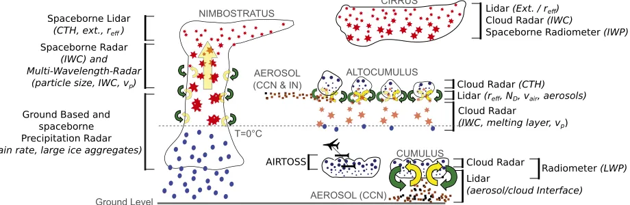
of the remote sensing campaigns that were performed within the last 20 years or are ongoing. The figure shows that ice-formation research is conducted globally and with significant efforts. An overview about the mea-surement campaigns inFig. 10-2is given inTable 10-1. Figure 10-3gives an overview about the objects and physical parameters that can be measured via remote sensing. From the climatological point of view, the most important parameters might be the ice water content (IWC), its corresponding ice water path (IWP), and the ice-effective radius (reff) because they have a large
in-fluence on the radiative transfer properties of an atmo-spheric volume. From the point of view of the actual ice-formation process, additionally, height level of ice formation, the corresponding temperature, and fall ve-locity might be most interesting because they tell where ice is formed and how it is evolving while falling through lower layers. FromFig. 10-3it can already be seen that the study of ice formation and evolution cannot be performed with a single instrument but only a combi-nation of several instruments and techniques can yield a clear picture.
b. Study of ice formation and evolution using ground-based lidar and radar
Ground-based lidars have been used for studying ice-formation processes (Ansmann et al. 2009a;Kanitz et al. 2011; see alsoFig. 10-2). While a lidar alone provides information about the presence of ice particles (Seifert et al. 2010), a combination of lidar and cloud radars can be used to quantify the amount of ice and water present in clouds (Hogan et al. 2006;Westbrook and Illingworth 2013;Bühl et al. 2016).
From the physical point of view, lidars and radars are similar instruments. Both transmit and receive electro-magnetic radiation, however, at different wavelengths. Lidars commonly operate in the optical (micrometer)
wavelength range, while cloud radars emit radiation in the microwave (millimeter) wavelength range. The ra-diation that is scattered back from ice particles is con-sequently proportional to D2 for lidars (geometrical scattering) and—for particles much smaller than the radar wavelength—D6for radars (Rayleigh scattering), withDindicating the volume-equivalent diameter of the particles. For particles larger than roughly 1/10th of the radar wavelength, the increase of backscattering with diameter is less thanD6, and other methods such as T matrix (Mishchenko 2000), Self-Similar Rayleigh–Gans (Hogan and Westbrook 2014), or the discrete dipole approximation (Draine and Flatau 1994) have to be used to estimate the backscattering of ice particles. Yet, the signals of both systems are strongly dominated by the largest particles in the observation volume. For radars, this effect is more dominant than for lidars. Therefore, a cloud radar is much better suited for the detection of large ice particles that appear in low numbers. However, a cloud radar can only partly detect the pre-dominantly liquid parts of the clouds where droplets are small but numerous. Here, the lidar backscatter signal is strongest but also strongly attenuated. As a conse-quence, a lidar can often not see though liquid cloud layers. The particle-detection capability of modern cloud radars is impressive, as a cloud radar with a sen-sitivity of 250 dBZ at cloud level can detect one co-lumnar ice particle with a length of about 200mm per cubic meter. Hence, the sensitivity is several magnitudes higher than, for example, that of typical precipitation radars, which have a typical lower signal threshold of about 0 dB. The higher sensitivity can be explained mainly by the closer range of observation (,12 km) and the shorter (millimeter range) wavelength. Airborne particle imagers would need long integration times in order to detect a significant amount of ice particles un-der such conditions. This illustrates the benefit of TABLE10-1. (Continued)
Campaign location Type
Duration (yr)
Data availability/website (if available)
Cheltenham [Facility for Airborne Atmospheric Measurements (FAAM)]
Small Particles in Cirrus (SPARTICUS) (aircraft)
,1 Zhang et al. (2013)
Cape Verde Ice in Clouds Experiment—Dust
(ICE-D) (aircraft)
,1 —
Svalbard Vertical Distribution of Ice in Arctic Mixed-Phase Clouds (VERDI) (aircraft)
,1 Klingebiel et al. (2015)
North Sea AIRTOSS campaign ,1 Finger et al. (2016)
Central Europe Midlatitude Cirrus Experiment (ML-CIRRUS)
,1 Voigt et al. (2017)
Central Amazonia ACRIDICON ,1 Wendisch et al. (2016)
[image:5.567.54.519.73.227.2]synergistic measurements of lidar and cloud radar in order to complement aircraft measurements under conditions of low ice concentrations. Prominent exam-ples of studies that employ combined approaches be-tween aircraft ground-based observations are Shupe et al. (2013)andWestbrook and Illingworth (2013).
Figure 10-3also highlights the importance of lidar and radar depolarization measurements for the identification and classification of ice particles. Depolarization in gen-eral is measured by emitting radiation in two perpendic-ular polarization states (dual-polarization method) or emitting in one polarization state and detecting in two. Dual-polarization methods have a long history for weather radars, because they can be used for the classifi-cation of hydrometeors (Thompson et al. 2014) or estimation of rain rates (Cifelli et al. 2011). Recently, dual-polarization methods for the size estimation of ice particles have also been implemented into cloud radars (Myagkov et al. 2016).Figure 10-4shows an example of a synergistic measurement result obtained from lidar, cloud radar, and microwave radiometer processed with the Cloudnet algorithm, which provides—among others— liquid water content (LWC) and IWC (Hogan et al. 2006). The lidar primarily detects the bases of liquid cloud layers, but also some of the ice particles falling from the mixed-phase cloud layer. Lidar depolarization shows low values at cloud top, where liquid particles dominate and high values in the virga. Liquid water path in the cloud top is measured with a microwave radiometer and scaled to the geometric extent of the liquid cloud layer (Fig. 10-4g). Ice water content is calculated using the aircraft-derived pa-rameterization ofHogan et al. (2006), which again high-lights the powerful combination of ground-based remote sensing observations with aircraft in situ measurements.
Measurements as shown inFig. 10-4can be generated automatically by state-of-the-art synergistic algorithms. However, they can only provide an overview of the dis-tribution of cloud particles and the height level of ice nu-cleation. The following evolution of a particle can be tracked using methods of fall-streak tracking (Marshall 1953).Hogan and Kew (2005)and Kalesse et al. (2016) showed how in situations when vertical wind shear is ob-served, the evolution of snow particles should be tracked along slanted fall streaks instead of considering vertical profiles. Other studies used the principle to observe hy-drometeors with high spatial resolution (Collier 1999) or to improve radar-derived rainfall estimations (Mittermaier et al. 2004;Lack and Fox 2007;Lauri et al. 2012).
Kalesse et al. (2016)assumed that the ice-formation process is stationary during cloud observation, and only additional information about the horizontal wind field is needed in order to follow particles through a cloud. Observation of the complete life cycle of ice particles from the level of ice formation toward ground level, which is possible by such techniques, is important, for example, in order to discriminate between primary ice formation or particle generation triggered by cloud-seeding effects.Figure 10-5shows an example of a fall streak tracked from the level of ice formation through a mixed-phase cloud system down to the ground where snowfall is detected. In this example, ice particles gen-erated near the top of the deep cloud frontal system are falling through a supercooled liquid layer where they experience riming and new ice particle formation hap-pens. The newly formed particles could either originate from ice multiplication (break up of rimed particles) or appear because of primary ice formation in the liquid layer (Zawadzki et al. 2001).
FIG. 10-3. Overview on remote sensing observation methods. For each cloud type, the height range is depicted that is optimal for the observation with ground and spaceborne lidar and radar systems and aircraft-tossed systems. The single systems (lidar, radar, microwave radiometer, and AIRTOSS) are explained in this section. Main properties of clouds derived from remote sensing measurements are cloud-top height (CTH), LWC/liquid water path (LWP), IWC, Doppler velocity of falling particles (yp), optical extinction (ext.), effective radius
[image:6.567.56.516.66.216.2]Additionally, Fig. 10-5 highlights the information content of the full cloud radar Doppler spectrum. As emphasized in Kollias et al. (2007), spectral Doppler information is expected to be one of the main tools for future observational studies on cloud microphysical properties. Several previous studies have demonstrated the potential of using multimodal cloud radar Doppler
spectra to characterize the liquid-phase and ice-phase components in mixed-phase clouds (e.g., Shupe et al. 2004; Luke et al. 2010;Jensen et al. 2010; Luke and Kollias 2013;Rambukkange et al. 2011;Verlinde et al. 2013;Kalesse et al. 2016). While lower moments of the radar spectrum (namely effective reflectivity Ze and mean Doppler velocity) are highly sensitive to the FIG. 10-4. Example of a combined lidar, cloud radar, and microwave radiometer measurement at Leipzig,
largest particles in the cloud volume detected by radar (as mentioned before Ze is proportional to D6), con-sidering the full Doppler spectrum enables detection of smaller particles with lower fall velocities. Doppler cloud radar observations with a high temporal and spectral resolution are required nevertheless, because the Doppler spectrum is also affected by dynamical ef-fects such as turbulence, which lead to spectral broad-ening and hamper microphysical retrievals (Babb et al. 1999;Scott et al. 2001). However, if sufficiently resolved, the Doppler velocity of the liquid cloud particles can be used as vertical air motion tracer. This approach is based on the assumption that the terminal velocity of small cloud droplets can be neglected compared to typical vertical air motions in clouds (Kollias et al. 2001). As an
alternative to the use of the full Doppler spectrum, the use of higher moments of the Doppler spectrum such as skewness and kurtosis as well as the slopes of the Doppler spectrum have been found useful for cloud observations (Luke and Kollias 2013;Maahn et al. 2015; Maahn and Löhnert 2017).
Recently, triple-frequency radar measurements in snowfall have the potential to give insight into ice particle characteristic size, habits, and ice particle density (Kneifel et al. 2014;Kulie et al. 2014).Kneifel et al. (2015) investigated relations between collocated ground-based triple-frequency radar observations (Ka, W, X band) in snowfall with in situ measurements performed at the ground. Concurrent analyses of two dual-wavelength ra-tios (i.e., the differences of the logarithmic effective radar FIG. 10-5. (a), (c) The reflectivity field of a 35-GHz zenith-pointing cloud radar in a wintertime deep frontal
reflectivity factor at two radar frequencies) at X/Ka band and Ka/W band were made. Clear signatures of snow particles with different characteristic sizes and densities (e.g., large low-density aggregates and heavily rimed snowflakes) could be distinguished in the triple-frequency space and were validated by the in situ mea-surements. As a further step,Kneifel et al. (2016)for the first time analyzed triple-frequency radar Doppler spec-tra in snowfall and showed that such sophisticated ob-servations can be used to validate snow scattering models. c. Spaceborne lidar and radar
TheCloudSatandCALIPSOsatellites were launched in 2006 to join the A-Train, a polar satellite family cur-rently consisting of six satellites in a sun-synchronous orbit that passes the equator at 1330 solar time and the ground track pattern repeats after approximately 16 days (Stephens et al. 2002). The Cloud Profiling Ra-dar (CPR) aboard CloudSat and the Cloud–Aerosol Lidar with Orthogonal Polarization (CALIOP) aboard CALIPSOare the first combination of active radar and lidar instruments in orbit specifically designed to glob-ally observe clouds and aerosols from space. The mea-sured signals from CPR and CALIOP are proportional to the amount of microwave (CPR) and infrared (CALIOP) radiation scattered back from hydrometeors in the atmosphere. The CALIOP lidar operates at a wavelength of 1064 nm and is therefore sensitive to small particles, while CPR, with its operation at 94 GHz (3-mm wavelength), is rather sensitive to larger and precipitating particles. Hence, CALIOP detects the thin cirrus clouds and cloud tops, and CPR probes thicker clouds and precipitation (Sassen et al. 2008), which cannot be penetrated by lidar. Their synergistic obser-vations are extensively used to study cloud formation and maintenance mechanisms (e.g.,Hogan and Illingworth 1999; Sato and Okamoto 2006; Sassen et al. 2008; Grenier et al. 2009;Sassen et al. 2009;Sassen and Zhu 2009;Wu et al. 2009;Yoshida et al. 2010;Zhang et al. 2010;Stein et al. 2011;Del Genio et al. 2012;Bühl et al. 2013;Battaglia and Delanoë2013).
Lidars suffer from attenuation by thick clouds, and because most lidars for aerosol and cloud detection are deployed on the ground (Pal et al. 1992;Van Tricht et al. 2014) their measurements can be obscured by low-level thick clouds (Thorsen et al. 2011). This problem is mitigated by CALIOP, which looks from above and is, therefore, well suited to retrieve cloud-top properties. In contrast to CALIOP, the CloudSat radar can even penetrate thick clouds. However,CloudSat’s CPR suf-fers from ground reflection that contaminates the ob-servations near the ground (Marchand et al. 2008; Maahn et al. 2014). Measurements close to the ground
are also challenging for vertically pointing ground-based radar systems because of detector saturation and other near-field effects (Görsdorf et al. 2015).
The raw power returns are converted into an equivalent attenuated reflectivity factor profile (CPR;Stephens et al. 2002) and attenuated backscatter profile (CALIOP; Winker et al. 2009). From these data products users can develop their own algorithms and products. Examples include the CloudSat radar–lidar geometrical profile product that provides vertical and spatial structure of hydrometeor layers based on combined CloudSat/ CALIPSO observations (Mace and Zhang 2014), the Combined Radar and Lidar Cloud Scenario Classifica-tion Product that includes informaClassifica-tion on cloud phase of the detected hydrometeor layers (Delanoë and Hogan 2008;Mace and Zhang 2014), and multiple data products with retrieved ice and liquid water contents and cloud optical depths (Austin et al. 2009;Vaughan et al. 2009;Winker et al. 2009;Deng et al. 2010).1
Algorithms have been developed and refined to take advantage of the nearly coincident satellite lidar and radar observations and combine the strengths of both systems (e.g.,Delanoëand Hogan 2010;Ceccaldi et al. 2013). Such data products provide vertically resolved profiles of cloud phase, and thus can be used to derive monthly cloud fraction data (Kay et al. 2008;Verlinden et al. 2011) and to determine aerosol–ice interactions and ice formation (Grenier et al. 2009). Furthermore, com-parisons against ice microphysical observations made by ground-based systems from the tropics to the poles (Protat et al. 2009,2010;Thorsen et al. 2011;Bromwich et al. 2012) can be performed. CALIOP data reveal the global cirrus cloud distribution (Sassen et al. 2008) and depolarization within ice clouds, with depolarization in-creasing at higher altitudes and dein-creasing with inin-creasing latitude (Sassen and Zhu 2009).
Reconciling differences between climatologies of, for ex-ample, heterogeneous ice formation calculated from ground-based observations with the corresponding results from satellite-based instruments is necessary for validation of satellite data products (Seifert et al. 2010;Kanitz et al. 2011;Bühl et al. 2013). The accuracy of many datasets over parts of Earth, such as the Southern Ocean, remains ques-tionable because of the lack of in situ measurements and the use of empirical relationships in the retrievals, which are derived from data in other locations. The correct represen-tation of ice in weather forecasting and general circulation models remains challenging, with over- and underestimates
1Publicly accessible data repositories forCloudSatandCALIPSO
can be found online at cloudsat.atmos.colostate.edu/data and
of ice compared withCALIPSOandCloudSatobservations in various regions of Earth and in different temperature regimes (Delanoëet al. 2011).
d. Microwave radiometers for measurement of atmospheric ice water path
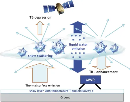
Microwave radiometry makes use of the interaction of microwave radiation (between 1 and 1000 GHz) with atmospheric gases and particles. While brightness tem-perature (TB) measurements along absorption lines are used for profiling of temperature and gases, window regions give insight into clouds and precipitation as they are semitransparent in this spectral region (see, e.g., Petty 2006). In general, extinction by water vapor and hydrometeors increases with frequency, with the stron-gest effect for ice clouds. Their effect can be neglected for frequencies below 60 GHz, enabling the retrieval of the liquid water path from multispectral measurements. However, with higher frequencies, both scattering cross section and absorption cross section of ice particles
strongly increase. The dominance of scattering leads to the fact that a layer of ice particles causes a TB depression for space-based observations because the thermal emission of the surface and lower atmospheric layers is scattered away (Fig. 10-6). This is the classical principle behind precipi-tation retrieval over land from millimeter-wave satellite observations (e.g., Grody 1991; Laviola and Levizzani 2011). For ground-based observations, however, scattering by ice particles leads to a brightness temperature increase, because the thermal emission of the relatively warm sur-face is scattered back to the radiometer.
The brightness temperature depression/increase (downward/upward pointing) is related to the integrated IWP (Evans et al. 1999,2005;Kneifel et al. 2010). Because the interaction between ice particles and microwave radiation depends to first order on the relation between particle size and wavelength, it is important that the se-lected microwave frequencies are sensitive to the ice particle size distribution. In this respect, passive micro-wave observations fill the gap between infrared (smallest FIG. 10-6. Illustration of the effects of liquid water and snow crystals on microwave TB measured at surface level and from space.
[image:10.567.56.507.66.418.2]particles) and radar (Fig. 10-7). Frequencies below 200 GHz are, therefore, mainly suited to sense snow while higher frequencies, that is, submillimeter wave-lengths, can be used to study ice clouds (Evans and Stephens 1995;Evans et al. 1999). However, not only ice scattering but also the continuum emission of liquid water and water vapor increases with frequency, which reduces the penetration depth with increasing frequen-cies. This is less of a problem for downward-pointing (satellite, high-flying aircraft) than upward-pointing ge-ometries as the surface contribution is omitted. From satellites the strong difference in opacity along water absorption lines can be exploited to infer the medium altitude of the ice cloud, that is, the height where IWP has reached half of its column value (Jiménez et al. 2007). Other ice particle properties like shape, density, and orientation also influence the microwave signal. For example, the preferentially horizontal orientation of snow particles (e.g., Pruppacher and Klett 1997) may cause a polarization difference (PD) of vertically and horizontally polarized brightness temperatures of more than 10 K for spaceborne observations (Gong and Wu 2017) and more than 8 K for ground-based observations (Xie et al. 2012) depending on aspect ratio. However, the strong absorption and emission of supercooled liq-uid water (SCLW) can mask PD for ground-based op-erations. For spaceborne operations, it instead depends on the geometry: if the SCLW is above oriented parti-cles, PD is reduced, while if it is below the ice layer, PD
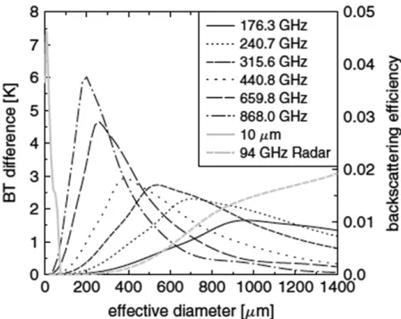
is actually enhanced (Xie et al. 2015). Also the presence of a melting layer can lead to an increased PD (Galligani et al. 2013; Gong and Wu 2017). IWP retrievals for current microwave satellite instruments exploiting the ice scattering signals for frequencies up to 190 GHz have been developed bySun and Weng (2012), among others, for the Special Sensor Microwave Imager/Sounder (SSM/IS) and Surussavadee and Staelin (2009) for the Advanced Microwave Sounding Unit (AMSU)/ Microwave Humidity Sounder (MHS). The Global Pre-cipitation Measurement (GPM;Hou et al. 2014) mission launched in 2014 aims to provide global spaceborne measurements of falling snow from both active and pas-sive microwave measurements, which both show a sen-sitivity threshold of about 0.5–1.0 mm h21 melted snow rate (Skofronick-Jackson et al. 2015). However, at these frequencies information is gathered mainly from snow particles (see Fig. 10-6) and the sensitivity to smaller particles typically found in ice clouds is low.Islam and Srivastava (2015)show how infrared observations, in this case High Resolution Infrared Radiation Sounder (HIRS), that are sensitive to much smaller particles complement the information of AMSU/MHS.Holl et al. (2014) developed the Synergistic Passive Atmospheric Retrieval Experiment-ICE (SPARE-ICE), which provides IWP combining Advanced Very High Resolution Radi-ometer (AVHRR) and MHS. They find a median fractional error between SPARE-ICE andCloudSatto be around a factor of 2, which is similar as the random error ofCloudSat IWC and in situ measurements. The suitability of the sub-millimeter region for ice cloud retrievals has already been demonstrated using limb sounding instruments mainly de-voted to stratospheric chemistry. Specifically, the Micro-wave Limb Sounder (MLS) (Waters et al. 2006) with channels at 240 and 640 GHz and the submillimeter radi-ometer (SMR) on board theOdinsatellite (Murtagh et al. 2002) with channels between 500 and 650 GHz provide in-formation on upper-tropospheric ice water content (Wu et al. 2008,Eriksson et al. 2014).
The gap in terms of global ice cloud and light snow climatologies will be closed by the Ice Cloud Imager (ICI) on MetOP-SG to be launched 2021 (Bergada et al. 2016). The ICI will carry channels featuring submillimeter fre-quencies ranging from 183 GHz up to 664 GHz with the frequencies 243 and 664 GHz featuring vertical and hor-izontal polarization. In addition to IWP, the ICI will also deliver the median mass equivalent sphere diameter and the median IWP altitude (Buehler et al. 2012). For process studies and prestudies for a satellite mission, air-borne sensors such as Compact Scanning Submillimeter-Wave Imaging Radiometer (CoSSIR;Evans et al. 2005), Conical Scanning Millimeter-Wave Imaging Radiom-eter (CoSMIR; Wang et al. 2007), and International FIG. 10-7. The sensitivity of measurements at various frequencies
to ice particle size. A fixed amount of cloud ice (IWP50.001 g m22)
and a narrow size distributions with differentDeffhave been used.
For eachDeff, the difference between clear-sky and cloudy radiance
is displayed. For comparison, the two gray curves show the size sensitivity for IR radiances at 10mm (solid), and for radar back-scatter measurements at 95 GHz (dashed). The right axis is for the radar curve, while the left axis is for all other curves. Figure from
[image:11.567.53.277.61.239.2]TB increase (Kneifel et al. 2010) and polarized mea-surements have been used to differentiate between mixed-phase and pure snowfall events and indicate the alignment of snow particles (Xie et al. 2012).
e. Passive remote sensing of cloud phase using solar spectral reflectivity
1) AIRBORNE RADIATION INSTRUMENTS
To measure cloud reflectivity, airborne radiation in-struments can be used, such as the Spectral Modular Air-borne Radiation Instrument (SMART) albedometer developed by Wendisch et al. (2001) and improved by Bierwirth et al. (2009), or the Solar Spectral Flux Radi-ometer (SSFR; Pilewskie et al. 2003). An overview of further airborne spectral radiation instruments and other airborne instrumentation is given by Wendisch et al. (2013b)andWendisch and Brenguier (2013). Several types of spectral radiance instruments are commonly used for ice identification measurements in clouds. On the one hand, pointing single-pixel spectrometers observe one pixel. On the other hand, multiangular imaging spectrometers ob-serve fields of pixels of the clouds. However, compared to pointing, single-pixel spectrometers, the wavelength reso-lutions of imaging spectrometers are often reduced and the opening angle is different. Prominent examples of com-mercially available imaging spectrometers are the Eagle and Hawk [push broom line imager, up to 1024 spatial pixel (608FOV), up to 1024 spectral pixel; see, e.g.,Schäfer et al. (2015)], charge-coupled device (CCD) cameras (Ehrlich et al. 2012), and polarization cameras.
2) ICE IDENTIFICATION USING CLOUD-REFLECTED RADIATION
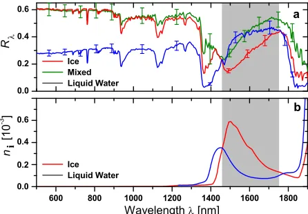
Figure 10-8 illustrates the basic principle of a method widely used to identify the ice phase in clouds, see, for ex-ample,Pilewskie and Twomey (1987),Ehrlich et al. (2008), Wendisch and Ehrlich (2011), and Jäkel et al. (2013). Figure 10-8bshows the spectrum of the absorption index (imaginary part of refractive indexni) for ice (red line) and
liquid water (blue line), respectively. In particular, in parts of the near-infrared (NIR) wavelength region (’1.4– 1.9mm) the maxima of the absorption indices are at different wavelengths, and the spectral slopes are also dif-ferent. These spectral features are reproduced in examples of cloud reflectivity spectra (Rl), shown in Fig. 10-8a. Cloud-reflected radiation spectra in the NIR exhibit a dis-tinctly different slope as a function of the ice content in the cloud; see the red (ice) and blue (liquid water) lines in Fig. 10-8a. Consequently, the slope of the cloud reflectivity spectra can be used to identify ice in mixed-phase clouds. The spectral slope ice indexIS is defined as the relative spectral slope of the measured reflectivity Rl at the two NIR wavelengths (l51700 and 1640 nm):IS5(R17002
R1640)/R1640. This ice indexIShas proven to be highly sen-sitive to spectral features of ice and liquid water absorption. From numerous simulations it is shown that values ofIS, 20 indicate a liquid water cloud, whereasIS’30 is repre-sentative for mixed-phase clouds, and larger values ofIS show the presence of ice clouds. A second ice index IS utilizes a principal component analysis of the spectral re-flectance in the same NIR wavelength range to distinguish ice and liquid water absorption in the measurements.
From the slope several realizations of ice indices can be derived that describe the phase composition of the cloud (Ehrlich et al. 2008). Unfortunately, no quantifi-cation of ice and liquid water content can be derived because of interferences with size and other parameters of the ice particles.
3) APPLICATION OF ICE INDEX TECHNIQUE Two example of ice index measurements are dis-cussed: The first one results from pointing, single-pixel FIG. 10-8. (a) Spectra of solar reflectivityRfor ice (red), mixed-phase (green), and liquid water (blue) clouds. The spectral range in which the spectral shapes are different is indicated by the gray areas. (b) Spectra of imaginary part of refractive indexnifor ice
[image:12.567.291.514.62.217.2]spectrometer measurements conducted above Arctic low-level clouds (Ehrlich et al. 2008); the second one stems from imaging spectrometer measurements of deep convective clouds in Amazonia (Wendisch et al. 2016).
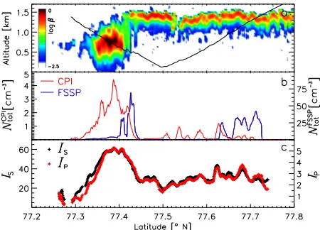
Ehrlich et al. (2008)calculated different realizations of the ice index from spectral reflectivity measurements conducted over Arctic low-level clouds (seeFig. 10-9). The two indicesIS andIP are derived from two tech-niques described in more detail byEhrlich et al. (2008). WhileISanalyzes the spectral slope of the reflectance in the NIR wavelength range,IPutilizes a principal com-ponent analysis (PCA) of the spectral reflectance. Figure 10-9cshows a time series of two of the derived ice indicesISandIP. Both ice indices show a similar relative course, the maximum coincides with a region where in situ measurements [Fig. 10-9b; cloud particle imager (CPI)] and lidar data (Fig. 10-9a) also indicate ice in the respective cloud portion. Furthermore, all three methods (ice index, in situ data, lidar) show a similar temporal evolution for mixed-phase clouds. The lidar profiles reveal that in the southern part of the cloud (left side ofFig. 10-9) ice particles are precipitating down to the surface. These precipitation particles, which are also observed from CloudSat (reflectivity) and can be de-tected by the lidar because they are not capped by a liquid water layer in this area.
[image:13.567.53.278.61.223.2]Wendisch et al. (2016) observed deep convective clouds over Amazonia by a side-viewing technique instead of looking from above at the cloud top (see
Fig. 10-10) during the Aerosol, Cloud, Precipitation, and Radiation Interactions and Dynamics of Convective Cloud Systems–Cloud Processes of the Main Precipitation Systems in Brazil: A Contribution to Cloud Resolving Modeling and to the GPM (ACRIDICON-CHUVA) campaign. In this case an imaging spectrometer was in-stalled inside the aircraft. The aircraft flies by (orbits) the cloud to obtain vertical profiles of the ice index. In Fig. 10-11, the NIR ice indices have been calculated from the spectra of the reflected radiation.Figure 10-11a shows the two-dimensional plots, Fig. 11b illustrates averages over the scene with indications of the height of the mixing layer. These measurements have been col-lected to obtain statistical data of the thickness and altitude of the mixed-phase layer in deep convective clouds and their dependence on aerosol and meteoro-logical conditions (for details, please see Wendisch et al. 2016).
4) COLLOCATED MEASUREMENT STRATEGY For a validation of the phase identification technique described above, collocated measurements of solar spec-tral radiation reflected by the clouds and concurrent in situ measurements of the cloud microphysics are ideal. Here two approaches are introduced: helicopterborne (Werner et al. 2013, 2014) and aircraftborne (Frey et al. 2009; Finger et al. 2016). Figure 10-12 illustrates both ap-proaches. For low clouds a slow-flying helicopter is used as an instrument carrier for Spectral Modular Airborne Radiation measurement system (SMART-HELIOS) and Airborne Cloud Turbulence Observation System (ACTOS) payloads. SMART-HELIOS takes spectral cloud reflectivity measurements from above the cloud to remotely sense the cloud ice; ACTOS does the micro-physical cloud sampling to indicate the cloud ice with in situ measurements inside the cloud. For high ice clouds, a fast-flying jet aircraft is used in combination with a towed measurement platform [Airborne Towed Sensor Shuttle (AIRTOSS)]. In this case the remote sensing of the ice in the clouds is done by spectral re-flectivity measurements on board the aircraft; the in situ verification is done by the AIRTOSS, which, by the way, contains not only a cloud microphysical in situ probe but also upward- and downward-looking solar spectral radiometers.
These collocated measurements have proven to be extremely valuable not only to verify remote sensing techniques to detect ice in clouds, but also to conduct studies of aerosol indirect radiative effects on cloud properties (Werner et al. 2014) and to perform collo-cated radiative budget measurements of clouds (Finger et al. 2016). But even if aircraft and in situ measurements are not collocated, they can be combined statistically: FIG. 10-9. Time series of different measurements obtained over
mixed-phase clouds in the Arctic (see Ehrlich et al. 2008). (a) Profile of total attenuated backscatter coefficientb[sr21km21]
measured byCALIPSOin a cloud observed on 7 Apr 2007. The flight track of the in situ measurements is overlaid as a black line. (b) Ice and liquid water particle concentrationsNtotmeasured by
Maahn et al. (2015)used the radar-derived relation be-tween radar reflectivity and mean Doppler velocity to-gether with aircraft in situ measurements in order to estimate the mass–size relation of arctic ice clouds as a function of temperature.
3. Conclusions and outlook
Active remotes sensing sensors like ground-based and spaceborne lidars and radars deliver direct informa-tion about the process of ice formainforma-tion. It has been shown that combined approaches—for example, aircraft
combined with active or passive remote sensing—can deliver a wealth of information. Passive optical obser-vations at cloud top with high resolution especially can provide instant information about the radiative prop-erties of a cloud, directly connecting the process level and the climatological impact. Methods like fall-streak tracking introduce a time component and allow tracing back the ice particles to their common point of origin.
The largest differences between ground-based and spaceborne systems are the scales that can be resolved in clouds; for example, ground-based cloud radars can re-solve about 50 m horizontally, and spaceborne radars
FIG. 10-11. Phase index derived from measurements of cloud-side reflected radiances for an example cloud. (a) Time series of vertical distribution of the phase index (side view), recorded during a flyby. The different colors represent values of the phase index. The dark gray areas indicate cloudless portions or land surface; the light gray areas represent shadow zones of the cloud sides, which are excluded from further analysis by an automatic cloud mask algorithm. These shadowed areas are not suitable for phase index analysis. The black vertical line indicates a dark-current measurement. (b) Vertical profile of phase index; three approximate altitudes (5.5, 7.6, and 11.7 km) are allocated to vertical pixels.
can resolve about 1000 m. Active ground-based systems can hence usually resolve the process length scales even of thin clouds (,300 m), while spaceborne systems still can, for example, observe the resulting ice mass. Re-cent developments of imaging systems spanning the infrared to ultraviolet wavelength range are about to go below the limit of 1000-m resolution (Cao et al. 2014). Such spaceborne measurements can provide a basic set of measurement variables that then can be used to infer indirect information about cloud processes via detailed modeling (Rosenfeld et al. 2014).Table 10-2 summa-rizes the advantages and disadvantages of the mea-surement systems described in this chapter and shows how passive and active optical and microwave obser-vation systems complement each other, in spite of their differences.
From Fig. 10-2, it seems as if there was a global coverage of remote sensing measurement campaigns, dedicated to ice formation. However, continuous long-term measurements are limited to a small band in the Northern Hemisphere with strong accumulations in central Europe and central North America. The dis-tribution of activities in the figure poses the question: Where to go next? There are obviously huge gaps in the global coverage of continuous active remote sensing measurements. However, such measurements are vital, for example, for the validation and ground truthing of combined remote sensing satellite missions (Illingworth et al. 2015). Also, the operational study of ice-formation processes is restricted to the meteoro-logical characteristics of the northern midlatitudes,
and there might be important variations on a regional scale. It becomes very clear that efforts have to be taken in order to enable continuous high-quality measurements also in regions of Earth that are less privileged. Efforts like the activities mentioned in Fig. 10-2 that took place, for example, at Manus, Nauru, northern Africa, or the central Amazonian rain forest have already gone into this direction. Such efforts should not be restricted to short-term cam-paign-like activities but should encompass long-term involvements in order to build up sustainable in-frastructure on site.
It appears as if the impact of single instrument ob-servations has diminished and the future of remote sensing research is built through synergistic multi-instrument and multiplatform approaches. The use of different methodologies (e.g., combinations of radar and lidar or in situ and remote sensing observations) allows for compensation of the limitations of a single measurement platform. Recently, scanning techniques with multiple radar instruments have been used to provide three-dimensional insight into cloud systems (Kollias et al. 2014) and multiwavelength techniques have become operationally applicable (Kneifel et al. 2011). For zenith-pointing radars, the use of the full Doppler spectrum opens new possibilities (Kollias et al. 2007). Lidars deliver more and more quantitative information about small cloud particles like cloud droplets (Donovan et al. 2015) or aerosol particles (Mamouri and Ansmann 2015), which are precursors for heterogeneous ice formation.
[image:15.567.127.440.59.287.2]Acknowledgments. We gratefully acknowledge the support from the Transregional Collaborative Re-search Center (TR 172) Arctic Amplification: Cli-mate Relevant Atmospheric and Surface Processes, and Feedback Mechanisms (AC)3, which is funded by the German Research Foundation (DFG, Deutsche Forschungsgemeinschaft). In addition, the authors would like to thank the many sponsors who have provided funding for the monograph: Leibniz Institute for Tropo-spheric Research (TROPOS), Forschungszentrum Jülich (FZJ), and Deutsches Zentrum für Luft- und Raumfahrt (DLR), Germany; ETH Zurich, Switzerland; National Center for Atmospheric Research (NCAR), United States; the Met Office, United Kingdom; the University of Illinois, United States; Environment and Climate Change Canada (ECCC), Canada; National Science Foundation (NSF), AGS 1723548, National Aeronautics and Space Administration (NASA), United States; the International Commission on Clouds and Precipitation (ICCP), the European Facility for Airborne Research (EUFAR), and Droplet Measurement Technologies (DMT), United States. NCAR is sponsored by the NSF. Any opinions, findings, and conclusions or recommendations expressed in this publication are those of the author(s) and do not necessarily reflect the views of the National Science Foundation.
REFERENCES
Anderson, T., and Coauthors, 2005: An ‘‘A-Train’’ strategy for quantifying direct climate forcing by anthropogenic aero-sols.Bull. Amer. Meteor. Soc.,86, 1795–1809, doi:10.1175/ BAMS-86-12-1795.
Ansmann, A., R. Engelmann, D. Althausen, U. Wandinger, M. Hu, Y. Zhang, and Q. He, 2005: High aerosol load over the Pearl River Delta, China, observed with Raman lidar and sun photometer. Geophys. Res. Lett.,32, L13815, doi:10.1029/2005GL023094. ——, H. Baars, M. Tesche, D. Müller, D. Althausen,
R. Engelmann, T. Pauliquevis, and P. Artaxo, 2009a: Dust and smoke transport from Africa to South America: Lidar pro-filing over Cape Verde and the Amazon rainforest.Geophys. Res. Lett.,36, L11802, doi:10.1029/2009GL037923.
——, and Coauthors, 2009b: Evolution of the ice phase in tropical altocumulus: SAMUM lidar observations over Cape Verde. J. Geophys. Res.,114, D17208, doi:10.1029/2008JD011659. Austin, R. T., A. J. Heymsfield, and G. L. Stephens, 2009: Retrieval
of ice cloud microphysical parameters using the CloudSat millimeter-wave radar and temperature.J. Geophys. Res.,114, D00A23, doi:10.1029/2008JD010049.
Babb, D. M., J. Verlinde, and B. A. Albrecht, 1999: Retrieval of cloud microphysical parameters from 94-GHz radar Doppler power spectra. J. Atmos. Oceanic Technol., 16, 489–503, doi:10.1175/1520-0426(1999)016,0489:ROCMPF.2.0.CO;2. Battaglia, A., and J. Delanoë, 2013: Synergies and complementarities
of CloudSat-CALIPSO snow observations. J. Geophys. Res. Atmos.,118, 721–731, doi:10.1029/2012JD018092.
Bergada, M., and Coauthors, 2016: The Ice Cloud Imager (ICI) preliminary design and performance.14th Specialist Meeting Satellites can provide global products for IWP Poor spatial resolution
Passive sensors Lightweight Nonspherical shapes (cirrus) (Eichler et al. 2009)
Portable Multilayer clouds (Werner et al. 2013)
Broadband/wide angle Cloud inhomogeneity effects (Schmidt et al. 2010;
Werner et al. 2014)
Sea ice and snow surfaces (Schäfer et al. 2015) Reflection–transmission (Brückner et al. 2014) Ground-based lidar Aerosol detection Strong attenuation in liquid layers
Detection of liquid layers Limited operation capabilities in precipitation Ground-based radar Suitable for detection and detailed analysis of
large particles
Detection of liquid layers difficult
Can penetrate thick clouds and precipitation Signal dominated by largest particles in observation volume
Can measure sedimentation velocity Spectrum reveals information about particle
on Microwave Radiometry and Remote Sensing of the Envi-ronment (MicroRad), Espoo, Finland, IEEE, doi:10.1109/ MICRORAD.2016.7530498.
Bierwirth, E., and Coauthors, 2009: Spectral surface albedo over Morocco and its impact on radiative forcing of Saharan dust. Tellus, 61B, 252–269, doi:10.1111/ j.1600-0889.2008.00395.x.
Bodas-Salcedo, A., and Coauthors, 2014: Origins of the solar ra-diation biases over the Southern Ocean in CFMIP2 models. J. Climate,27, 41–56, doi:10.1175/JCLI-D-13-00169.1. Bromwich, D. H., and Coauthors, 2012: Tropospheric clouds
in Antarctica. Rev. Geophys., 50, RG1004, doi:10.1029/ 2011RG000363.
Brückner, M., A. Pospichal, A. Macke, and M. Wendisch, 2014: A new multispectral cloud retrieval method for ship-based solar transmissivity measurements.J. Geophys. Res. Atmos.,119, 11 338–11 354, doi:10.1002/2014JD021775.
Buehler, S. A., and Coauthors, 2007: A concept for a satellite mission to measure cloud ice water path, ice particle size, and cloud altitude.Quart. J. Roy. Meteor. Soc., 133, 109–128, doi:10.1002/qj.143.
——, and Coauthors, 2012: Observing ice clouds in the sub-millimeter spectral range: The CloudIce mission proposal for ESA’s Earth Explorer 8.Atmos. Meas. Tech.,5, 1529–1549, doi:10.5194/amt-5-1529-2012.
Bühl, J., A. Ansmann, P. Seifert, H. Baars, and R. Engelmann, 2013: Toward a quantitative characterization of heterogeneous ice formation with lidar/radar: Comparison of CALIPSO/ CloudSat with ground-based observations.Geophys. Res. Lett., 40, 4404–4408, doi:10.1002/grl.50792.
——, P. Seifert, A. Myagkov, and A. Ansmann, 2016: Measuring ice- and liquid-water properties in mixed-phase cloud layers at the Leipzig Cloudnet station.Atmos. Chem. Phys.,16, 10 609– 10 620, doi:10.5194/acp-16-10609-2016.
Cao, C., S. Blonski, W. Wang, X. Shao, T. Choi, Y. Bai, and X. Xiong, 2014: Overview of Suomi NPP VIIRS performance in the last 2.5 years.Earth Observing Missions and Sensors: Development, Implementation, and Characterization III, X. Xiong and H. Shimoda, Eds., International Society for Optical Engineering (SPIE Proceedings, Vol. 9264), 926402, doi:10.1117/12.2068991. Ceccaldi, M., J. Delanoë, R. J. Hogan, N. L. Pounder, A. Protat, and J. Pelon, 2013: From CloudSat-CALIPSO to EarthCare: Evolution of the DARDAR cloud classification and its com-parison to airborne radar-lidar observations.J. Geophys. Res. Atmos.,118, 7962–7981, doi:10.1002/jgrd.50579.
Cifelli, R., V. Chandrasekar, S. Lim, P. C. Kennedy, Y. Wang, and S. A. Rutledge, 2011: A new dual-polarization radar rainfall algorithm: Application in Colorado precipitation events. J. Atmos. Oceanic Technol., 28, 352–364, doi:10.1175/ 2010JTECHA1488.1.
Cohen, J., and Coauthors, 2014: Recent Arctic amplification and extreme mid-latitude weather. Nat. Geosci., 7, 627–637, doi:10.1038/ngeo2234.
Collier, C. G., 1999: The impact of wind drift on the utility of very high spatial resolution radar data over urban areas.Phys. Chem. Earth,24B, 889–893, doi:10.1016/S1464-1909(99)00099-4. Delanoë, J., and R. J. Hogan, 2008: A variational scheme for
re-trieving ice cloud properties from combined radar, lidar, and infrared radiometer. J. Geophys. Res., 113, D07204, doi:10.1029/2007JD009000.
——, and ——, 2010: Combined CloudSat-CALIPSO-MODIS retrievals of the properties of ice clouds.J. Geophys. Res., 115, D00H29, doi:10.1029/2009JD012346.
——, ——, R. M. Forbes, A. Bodas-Salcedo, and T. H. M. Stein, 2011: Evaluation of ice cloud representation in the ECMWF and Met Office models using CloudSat and CALIPSO data. Quart. J. Roy. Meteor. Soc.,137, 2064–2078, doi:10.1002/qj.882. Del Genio, A. D., Y. Chen, D. Kim, and M.-S. Yao, 2012: The MJO transition from shallow to deep convection in CloudSat/ CALIPSO data and GISS GCM simulations.J. Climate,25, 3755–3770, doi:10.1175/JCLI-D-11-00384.1.
Deng, M., G. G. Mace, Z. Wang, and H. Okamoto, 2010: Tropical Composition, Cloud and Climate Coupling Experiment valida-tion for cirrus cloud profiling retrieval using CloudSat radar and CALIPSO lidar. J. Geophys. Res., 115, D00J15, doi:10.1029/ 2009JD013104.
Donovan, D. P., H. Klein Baltink, J. S. Henzing, S. R. De Roode, and A. P. Siebesma, 2015: A depolarisation lidar-based method for the determination of liquid-cloud microphysical properties. Atmos. Meas. Tech.,8, doi:10.5194/amt-8-237-2015.
Draine, B. T., and P. J. Flatau, 1994: Discrete-dipole approxima-tion for scattering calculaapproxima-tions.J. Opt. Soc. Amer.,11A, 1491, doi:10.1364/JOSAA.11.001491.
Ehrlich, A., E. Bierwirth, M. Wendisch, J.-F. Gayet, G. Mioche, A. Lampert, and J. Heintzenberg, 2008: Cloud phase identifi-cation of Arctic boundary-layer clouds from airborne spectral reflection measurements: Test of three approaches. Atmos. Chem. Phys.,8, 7493–7505, doi:10.5194/acp-8-7493-2008. ——, ——, ——, A. Herber, and J.-F. Gayet, 2012: Airborne
hy-perspectral observations of surface and cloud directional re-flectivity using a commercial digital camera. Atmos. Chem. Phys.,12, 3493–3510, doi:10.5194/acp-12-3493-2012. Eichler, H., A. Ehrlich, M. Wendisch, G. Mioche, J.-F. Gayet,
M. Wirth, C. Emde, and A. Minikin, 2009: Influence of ice crystal shape on retrieval of cirrus optical thickness and ef-fective radius: A case study.J. Geophys. Res.,114, D19203, doi:10.1029/2009JD012215.
Eriksson, P., B. Rydberg, H. Sagawa, M. S. Johnston, and Y. Kasai, 2014: Overview and sample applications of SMILES and Odin-SMR retrievals of upper tropospheric humidity and cloud ice mass. Atmos. Chem. Phys., 14, 12 613–12 629, doi:10.5194/acp-14-12613-2014.
Evans, K. F., and G. L. Stephens, 1995: Microwave radiative transfer through clouds composed of realistically shaped ice crystals. Part I. Single scattering properties.J. Atmos. Sci.,52, 2041–2057, doi:10.1175/1520-0469(1995)052,2041:MRTTCC.2.0.CO;2. ——, A. H. Evans, I. G. Nolt, and B. T. Marshall, 1999: The prospect
for remote sensing of cirrus clouds with a submillimeter-wave spectrometer. J. Appl. Meteor., 38, 514–525, doi:10.1175/ 1520-0450(1999)038,0514:TPFRSO.2.0.CO;2.
——, J. R. Wang, P. E. Racette, G. Heymsfield, and L. Li, 2005: Ice cloud retrievals and analysis with the compact scanning sub-millimeter imaging radiometer and the cloud radar system during CRYSTAL FACE. J. Appl. Meteor., 44, 839–859, doi:10.1175/JAM2250.1.
Fan, J., Y. Wang, D. Rosenfeld, and X. Liu, 2016: Review of aerosol– cloud interactions: Mechanisms, significance, and challenges. J. Atmos. Sci.,73, 4221–4252, doi:10.1175/JAS-D-16-0037.1. Finger, F., and Coauthors, 2016: Spectral optical layer properties
of cirrus from collocated airborne measurements and simu-lations. Atmos. Chem. Phys., 16, 7681–7693, doi:10.5194/ acp-16-7681-2016.
Gong, J., and D. L. Wu, 2017: Microphysical properties of frozen particles inferred from Global Precipitation Measurement (GPM) Microwave Imager (GMI) polarimetric measure-ments. Atmos. Chem. Phys., 17, 2741–2757, doi:10.5194/ acp-17-2741-2017.
Gorodetskaya, I. V., and Coauthors, 2015: Cloud and precip-itation properties from ground-based remote-sensing in-struments in East Antarctica. Cryosphere, 9, 285–304, doi:10.5194/tc-9-285-2015.
Görsdorf, U., V. Lehmann, M. Bauer-Pfundstein, G. Peters, D. Vavriv, V. Vinogradov, and V. Volkov, 2015: A 35-GHz polarimetric Doppler radar for long-term observations of cloud parameters—Description of system and data processing. J. Atmos. Oceanic Technol., 32, 675–690, doi:10.1175/ JTECH-D-14-00066.1.
Grenier, P., J. Blanchet, and R. Muñoz-Alpizar, 2009: Study of polar thin ice clouds and aerosols seen by CloudSat and CALIPSO during midwinter 2007. J. Geophys. Res., 114, D09201, doi:10.1029/2008JD010927.
Grody, N. C., 1991: Classification of snow cover and precipitation using the special sensor microwave imager.J. Geophys. Res., 96, 7423–7435, doi:10.1029/91JD00045.
Heintzenberg, J., 2009: The SAMUM-1 experiment over Southern Morocco: Overview and introduction. Tellus, 61B, 2–11, doi:10.1111/j.1600-0889.2008.00403.x.
Heymsfield, A. J., P. R. Field, M. Bailey, D. Rogers, J. Stith, C. Twohy, Z. Wang, and S. Haimov, 2011: Ice in Clouds Experiment—Layer Clouds. Part I: Ice growth rates derived from lenticular wave cloud penetrations.J. Atmos. Sci.,68, 2628–2654, doi:10.1175/JAS-D-11-025.1.
Hogan, R. J., and A. J. Illingworth, 1999: The potential of space-borne dual-wavelength radar to make global measurements of cirrus clouds. J. Atmos. Oceanic Technol., 16, 518–531, doi:10.1175/1520-0426(1999)016,0518:TPOSDW.2.0.CO;2. ——, and S. F. Kew, 2005: A 3D stochastic cloud model for
in-vestigating the radiative properties of inhomogeneous cirrus clouds.Quart. J. Roy. Meteor. Soc.,131, 2585–2608, doi:10.1256/ qj.04.144.
——, and C. D. Westbrook, 2014: Equation for the microwave backscatter cross section of aggregate snowflakes using the self-similar Rayleigh–Gans approximation.J. Atmos. Sci.,71, 3292–3301, doi:10.1175/JAS-D-13-0347.1.
——, M. P. Mittermaier, and A. J. Illingworth, 2006: The retrieval of ice water content from radar reflectivity factor and tem-perature and its use in evaluating a mesoscale model.J. Appl. Meteor. Climatol.,45, 301–317, doi:10.1175/JAM2340.1. Holl, G., S. Eliasson, J. Mendrok, and S. A. Buehler, 2014:
SPARE-ICE: Synergistic ice water path from passive operational
doi:10.1175/BAMS-88-6-883.
——, and Coauthors, 2015: The EarthCARE satellite: The next step forward in global measurements of clouds, aerosols, precipitation, and radiation. Bull. Amer. Meteor. Soc., 96, 1311–1332, doi:10.1175/BAMS-D-12-00227.1.
Islam, T., and P. K. Srivastava, 2015: Synergistic multi-sensor and multi-frequency retrieval of cloud ice water path constrained by CloudSat collocations.J. Quant. Spectrosc. Radiat. Trans-fer,161, 21–34, doi:10.1016/j.jqsrt.2015.03.022.
Jäkel, E., J. Walter, and M. Wendisch, 2013: Thermodynamic phase retrieval of convective clouds: Impact of sensor viewing geo-metry and vertical distribution of cloud properties.Atmos. Meas. Tech.,6, 539–547, doi:10.5194/amt-6-539-2013. Jensen, E. J., L. Pfister, T. P. Bui, P. Lawson, and D. Baumgardner,
2010: Ice nucleation and cloud microphysical properties in tropical tropopause layer cirrus. Atmos. Chem. Phys., 10, 1369–1384, doi:10.5194/acp-10-1369-2010.
Jiménez, C., S. A. Buehler, B. Rydberg, P. Eriksson, and K. F. Evans, 2007: Performance simulations for a submillimeter-wave satellite instrument to measure cloud ice.Quart. J. Roy. Meteor. Soc.,133, 129–149, doi:10.1002/qj.134.
Kalesse, H., W. Szyrmer, S. Kneifel, P. Kollias, and E. Luke, 2016: Fingerprints of a riming event on cloud radar Doppler spectra: Observations and modeling.Atmos. Chem. Phys.,16, 2997– 3012, doi:10.5194/acp-16-2997-2016.
Kanitz, T., P. Seifert, A. Ansmann, R. Engelmann, D. Althausen, C. Casiccia, and E. G. Rohwer, 2011: Contrasting the impact of aerosols at northern and southern midlatitudes on heteroge-neous ice formation. Geophys. Res. Lett., 38, L17802, doi:10.1029/2011GL048532.
Kay, J. E., T. L’Ecuyer, A. Gettelman, G. L. Stephens, and C. O’Dell, 2008: The contribution of cloud and radiation anomalies to the 2007 Arctic sea ice extent minimum. Geo-phys. Res. Lett.,35, L08503, doi:10.1029/2008GL033451. Klingebiel, M., and Coauthors, 2015: Arctic low-level boundary
layer clouds: In situ measurements and simulations of mono-and bimodal supercooled droplet size distributions at the top layer of liquid phase clouds.Atmos. Chem. Phys.,15, 617–631, doi:10.5194/acp-15-617-2015.
Kneifel, S., U. Löhnert, A. Battaglia, S. Crewell, and D. Siebler, 2010: Snow scattering signals in ground-based passive micro-wave radiometer measurements.J. Geophys. Res. Atmos.,115, D16214, doi:10.1029/2010JD013856.
——, M. S. Kulie, and R. Bennartz, 2011: A triple-frequency ap-proach to retrieve microphysical snowfall parameters. J. Geophys. Res.,116, D11203, doi:10.1029/2010JD015430. ——, S. Redl, E. Orlandi, U. Löhnert, M. P. Cadeddu, D. D. Turner,
liquid water between 31 and 225 GHz: Evaluation of absorption models using ground-based observations.J. Appl. Meteor. Cli-matol.,53, 1028–1045, doi:10.1175/JAMC-D-13-0214.1. ——, A. von Lerber, J. Tiira, D. Moisseev, P. Kollias, and
J. Leinonen, 2015: Observed relations between snowfall mi-crophysics and triple-frequency radar measurements. J. Geophys. Res. Atmos., 120, 6034–6055, doi:10.1002/ 2015JD023156.
——, P. Kollias, A. Battaglia, J. Leinonen, M. Maahn, H. Kalesse, and F. Tridon, 2016: First observations of triple-frequency radar Doppler spectra in snowfall: Interpretation and appli-cations. Geophys. Res. Lett., 43, 2225–2233, doi:10.1002/ 2015GL067618.
Kollias, P., B. A. Albrecht, and F. D. Marks, 2001: Raindrop sorting induced by vertical drafts in convective clouds.Geophys. Res. Lett.,28, 2787–2790, doi:10.1029/2001GL013131.
——, E. E. Clothiaux, M. A. Miller, B. A. Albrecht, G. L. Stephens, and T. P. Ackerman, 2007: Millimeter-wavelength radars. Bull. Amer. Meteor. Soc., 88, 1608–1624, doi:10.1175/ BAMS-88-10-1608.
——, N. Bharadwaj, K. Widener, I. Jo, and K. Johnson, 2014: Scanning ARM cloud radars. Part I: Operational sampling strategies.J. Atmos. Oceanic Technol.,31, 569–582, doi:10.1175/ JTECH-D-13-00044.1.
Kulie, M. S., M. J. Hiley, R. Bennartz, S. Kneifel, and S. Tanelli, 2014: Triple-frequency radar reflectivity signatures of snow: Observations and comparisons with theoretical ice particle scattering models.J. Appl. Meteor. Climatol.,53, 1080–1098, doi:10.1175/JAMC-D-13-066.1.
Lack, S. A., and N. I. Fox, 2007: An examination of the effect of wind drift on radar-derived surface rainfall estimations. At-mos. Res.,85, 217–229, doi:10.1016/j.atmosres.2006.09.010. Lauri, T., J. Koistinen, and D. Moisseev, 2012: Advection-based
adjustment of radar measurements. Mon. Wea. Rev., 140, 1014–1022, doi:10.1175/MWR-D-11-00045.1.
Laviola, S., and V. Levizzani, 2011: The 183-WSL fast rain rate retrieval algorithm: Part I: Retrieval design.Atmos. Res.,99, 443–461, doi:10.1016/j.atmosres.2010.11.013.
Lohmann, U., F. Lüönd, and F. Mahrt, 2016: Introduction to Clouds: From the Microscale to Climate.Cambridge Univer-sity Press, 399 pp., doi:10.1017/CBO9781139087513. Löhnert, U., S. Kneifel, A. Battaglia, M. Hagen, L. Hirsch, and
S. Crewell, 2011: A multisensor approach toward a better understanding of snowfall microphysics: The TOSCA project.Bull. Amer. Meteor. Soc.,92, 613–628, doi:10.1175/ 2010BAMS2909.1.
Luke, E. P., and P. Kollias, 2013: Separating cloud and drizzle radar moments during precipitation onset using Doppler spectra. J. Atmos. Oceanic Technol., 30, 1656–1671, doi:10.1175/ JTECH-D-11-00195.1.
——, ——, and M. D. Shupe, 2010: Detection of supercooled liquid in mixed-phase clouds using radar Doppler spectra. J. Geophys. Res.,115, D19201, doi:10.1029/2009JD012884. Maahn, M., and U. Löhnert, 2017: Potential of higher order
moments of the radar Doppler spectrum for retrieving mi-crophysical and kinematic properties of Arctic ice clouds. J. Appl. Meteor. Climatol., 56, 263–282, doi:10.1175/ JAMC-D-16-0020.1.
——, C. Burgard, S. Crewell, I. V. Gorodetskaya, S. Kneifel, S. Lhermitte, K. Van Tricht, and N. P. M. van Lipzig, 2014: How does the spaceborne radar blind zone affect derived surface snowfall statistics in polar regions?J. Geophys. Res. Atmos.,119, 13 604–13 620, doi:10.1002/2014JD022079.
——, U. Löhnert, P. Kollias, R. C. Jackson, and G. M. McFarquhar, 2015: Developing and evaluating ice cloud parameterizations for forward modeling of radar moments using in situ air-craft observations.J. Atmos. Oceanic Technol.,32, 880–903, doi:10.1175/JTECH-D-14-00112.1.
Mace, G. G., and Q. Zhang, 2014: The CloudSat radar-lidar geo-metrical profile product (RL-GeoProf): Updates, improve-ments, and selected results. J. Geophys. Res. Atmos., 119, 9441–9462, doi:10.1002/2013JD021374.
Mamouri, R. E., and A. Ansmann, 2015: Estimated desert-dust ice nuclei profiles from polarization lidar: Methodology and case studies. Atmos. Chem. Phys., 15, 3463–3477, doi:10.5194/ acp-15-3463-2015.
Marchand, R., G. G. Mace, T. Ackerman, and G. Stephens, 2008: Hydrometeor detection using Cloudsat—An Earth-orbiting 94-GHz cloud radar.J. Atmos. Oceanic Technol.,25, 519–533, doi:10.1175/2007JTECHA1006.1.
——, T. Ackerman, M. Smyth, and W. B. Rossow, 2010: A review of cloud top height and optical depth histograms from MISR, ISCCP, and MODIS. J. Geophys. Res., 115, D16206, doi:10.1029/2009JD013422.
Marshall, J. S., 1953: Precipitation trajectories and patterns. J. Meteor.,10, 25–29, doi:10.1175/1520-0469(1953)010,0025: PTAP.2.0.CO;2.
Mather, J. H., and J. W. Voyles, 2013: The ARM Climate Research Facility: A review of structure and capabilities.Bull. Amer. Meteor. Soc.,94, 377–392, doi:10.1175/BAMS-D-11-00218.1. May, P. T., J. H. Mather, G. Vaughan, C. Jakob, G. M.
McFarquhar, K. N. Bower, and G. G. Mace, 2008: The Trop-ical Warm Pool International Cloud Experiment.Bull. Amer. Meteor. Soc.,89, 629, doi:10.1175/BAMS-89-5-629.
Miller, M. A., K. Nitschke, T. P. Ackerman, W. R. Ferrell, N. Hickmon, and M. Ivey, 2016: The ARM Mobile Facilities. The Atmospheric Radiation Measurement (ARM) Program: The First 20 Years,Meteor. Monogr., No. 57, Amer. Meteor. Soc., doi:10.1175/AMSMONOGRAPHS-D-15-0051.1. Mishchenko, M. I., 2000: Calculation of the amplitude matrix for a
nonspherical particle in a fixed orientation.Appl. Opt.,39, 1026–1031, doi:10.1364/AO.39.001026.
Mittermaier, P. M., J. R. Hogan, and J. A. Illingworth, 2004: Using mesoscale model winds for correcting wind-drift errors in ra-dar estimates of surface rainfall.Quart. J. Roy. Meteor. Soc., 130, 2105–2123, doi:10.1256/qj.03.156.
Morrison, H., G. de Boer, G. Feingold, J. Harrington, M. D. Shupe, and K. Sulia, 2012: Resilience of persistent Arctic mixed-phase clouds.Nat. Geosci.,5, 11–17, doi:10.1038/ngeo1332. Murtagh, D., and Coauthors, 2002: An overview of the Odin
at-mospheric mission.Can. J. Phys.,80, 309–319, doi:10.1139/ p01-157.
Myagkov, A., P. Seifert, U. Wandinger, M. Bauer-Pfundstein, and S. Y. Matrosov, 2015: Effects of antenna patterns on cloud radar polarimetric measurements.J. Atmos. Oceanic Technol., 32, 1813–1828, doi:10.1175/JTECH-D-15-0045.1.
——, ——, M. Bauer-Pfundstein, and U. Wandinger, 2016: Cloud radar with hybrid mode towards estimation of shape and ori-entation of ice crystals. Atmos. Meas. Tech., 9, 469–489, doi:10.5194/amt-9-469-2016.
Naud, C., J. F. Booth, and A. D. Del Genio, 2014: Evaluation of ERA-Interim and MERRA cloudiness in the Southern Ocean. J. Climate,27, 2109–2124, doi:10.1175/JCLI-D-13-00432.1. Pal, S. R., W. Steinbrecht, and A. I. Carswell, 1992: Automated