Consistent dirichlet boundary conditions for numerical solution of moving boundary problems

(1)

This is a repository copy of Consistent dirichlet boundary conditions for numerical solution

of moving boundary problems.

White Rose Research Online URL for this paper: http://eprints.whiterose.ac.uk/8483/

Article:

Hubbard, M.E., Baines, M.J. and Jimack, P.K. (2009) Consistent dirichlet boundary conditions for numerical solution of moving boundary problems. Applied Numerical Mathematics, 59 (6). pp. 1337-1353. ISSN 01689274

https://doi.org/10.1016/j.apnum.2008.08.002

[email protected] https://eprints.whiterose.ac.uk/ Reuse

See Attached

Takedown

If you consider content in White Rose Research Online to be in breach of UK law, please notify us by

(2)

Consistent Dirichlet Boundary Conditions for Numerical

Solution of Moving Boundary Problems

M.E.Hubbard, M.J.Baines, P.K.Jimack

August 7, 2008

Abstract

We consider the imposition of Dirichlet boundary conditions in the finite element mod-elling of moving boundary problems in one and two dimensions for which the total mass is prescribed. A modification of the standard linear finite element test space allows the bound-ary conditions to be imposed strongly whilst simultaneously conserving a discrete mass. The validity of the technique is assessed for a specific moving mesh finite element method, although the approach is more general. Numerical comparisons are carried out for mass-conserving solutions of the porous medium equation with Dirichlet boundary conditions and for a moving boundary problem with a source term and time-varying mass.

1 Introduction

Moving boundary problems are very common in the mathematical modelling of physical processes [12]. Compared with fixed boundary problems they require extra boundary condi-tions to determine the motion of the boundary. For example, standard Dirichlet condicondi-tions for a fixed boundary problem are often supplemented by additional Neumann conditions. An appropriate discretisation for these problems is the finite element method with moving nodes, and many such techniques have been proposed in recent years [1, 3, 7, 8, 9, 10, 13, 15]. It should be noted however that the additional boundary conditions required to ensure well-posedness of the moving boundary problem introduce extra constraints on the treatment of the finite element equations at the boundary. In this paper we discuss the imposition of strong constraints (specifically, Dirichlet boundary conditions) on sets of moving mesh finite element equations with constraints on the total mass.

Solutions of these problems often exhibit global properties such as mass conservation,

i.e. the preservation of an integral of the dependent variable in time. Such properties are

(3)

and disregard the finite element equations arising from the test functions associated with those nodes. However, this step also destroys mass conservation in general, which may be a key property.

In this paper we discuss ways of preserving both Dirichlet conditions and conservation of mass by a modification of the test space. The procedure is described in the context of schemes which use a general ALE (Arbitrary Lagrangian-Eulerian) framework, after which a computational assessment is undertaken for one such scheme [1, 2]. In the remainder of this section we describe the class of moving boundary problems and boundary conditions consid-ered here. A general form of the moving mesh finite element equations is then stated and the problem of simultaneously implementing Dirichlet boundary conditions and conservation is discussed. In the following section, ways of overcoming these problems are described, in both one and two space dimensions. The resulting algorithm is then tested on a selection of problems in one and two dimensions, using the moving mesh finite element method given in [1, 2]. We conclude with a short discussion.

1.1 Moving Boundary Problems and ALE Finite Elements

Consider a moving boundary problem of the form

ut = ∇ · Fu for x∈ R(t), (1)

where F is a spatial operator, with Dirichlet boundary conditions u = g on the moving

boundary ∂R(t). We shall mainly be concerned with problems for which the total mass,

Z

R₍t)

u(t,x)dx, (2)

remains constant in time: this class of problems includes a wide variety of nonlinear diffusion equations [1, 3, 6, 12]. However, as will be demonstrated, the ideas presented will apply to more general problems too.

By the Reynolds Transport Theorem [14] and (1),

d dt

Z

R₍t)

u(t,x)dx =

Z

R₍t)

utdx+

I

∂R₍t)

uv·ndS

=

Z

R(t)

∇ · Fu dx+

I

∂R(t)

uv·ndS

=

I

∂R₍t)

(Fu+uv)·ndS (3)

where v(t) is the velocity of the boundary. Thus, the total mass (2) is conserved if and only

if the boundary integral in (3) is zero. This, in turn, is true if u and vsatisfy the boundary

condition

(4)

Now consider a piecewise linear moving mesh finite element approach based upon a weak

form of the Reynolds Transport Theorem. In order to do this let Ω(t) be a moving polygonal

approximation toR(t) and assume a moving triangulation of Ω(t) with N+B vertices, the

first N being in the interior and the remainder being on the moving boundary. Let the test

functions Wi(t,x), (i= 1, ..., N+B), be piecewise linear basis functions forming a partition

of unity, and define piecewise linear approximations, U ≈uand V≈v, in the moving frame

by

U(t,x) =

N_X+B j=1

Uj(t)Wj(t,x), V(t,x) =

N_X+B j=1

Vj(t)Wj(t,x) (5)

(for further details see [1]). Then (cf.(3))

d dt

Z

Ω(t)

Wi(t,x)U(t,x)dx =

Z

Ω(t)

∂

∂t (WiU) dx+ I

∂Ω(t)

WiUV·ndS

=

Z

Ω(t)

Wi∇ ·(FU)dx+

Z

Ω(t)

Wi∇ ·(UV)dx

=

Z

Ω(t)

Wi∇ ·(FU+UV) dx (6)

for i = 1, ..., N +B, using (1) and the divergence theorem. Note that the second equality

above uses the fact that the test functionWi moves withV(i.e.satisfies∂Wi/∂t+V·∇Wi =

0), as shown in [1] for example, and U is regularised as necessary to lie in the domain of F.

Using integration by parts on (6), assuming that the discrete form of the boundary con-dition (4) holds on the boundary, the ALE finite element form is

d dt

Z

Ω(t)

Wi(t,x)U(t,x)dx = −

Z

Ω(t)

∇Wi·(FU +UV) dx. (7)

AnyVwhich satisfies the discrete form of (4) can be used in (7), leading via time-integration

to the specification of _Z

Ω(t)

Wi(t,x)U(t,x)dx (8)

and subsequently to the evaluation of U(t,x) (see below). It is the imposition of boundary

conditions on this quantity that is the subject of this paper.

1.2 Mass Conservation

Note that the total discrete mass is given by

Z

Ω(t)

U(t,x)dx. (9)

Furthermore, summing equations (7) over i= 1, ..., N +B yields

d dt

Z

Ω(t)

(5)

since the functions Wi(t,x) form a partition of unity on Ω(t); that is P_iN₌₁+BWi(t,x) ≡ 1

for all t. This implies that for any ALE finite element method of the form (7), which is

constrained to satisfy the discrete form of (4) on the whole boundary, we obtain discrete mass conservation.

However, this argument holds only for weak imposition of Dirichlet boundary conditions

on U. When Dirichlet boundary conditions are imposed strongly the test functions Wi(t,x)

no longer form a partition of unity, since (7) only holds for i = 1, ..., N, and so summation

of these equations no longer yields conservation of the total discrete mass. In Section 2 below we describe a technique for modifying this test space which allows Dirichlet boundary conditions to be imposed strongly whilst simultaneously maintaining discrete conservation of mass.

In order to simplify the description of this technique we shall present it for one specific choice of ALE finite element method, that described in [1] (see below). However, the gener-alisation to any ALE solver is straightforward and is described in the Discussion at the end of this paper. For completeness a brief outline of the method of [1] is provided in Appendix

A. The idea upon which it is based is to drive the mesh movement according to adistributed

conservation principle _Z

Ω(t)

Wi(t,x)U(t,x)dx = Ci, (11)

where each Ci is a constant in time, retaining its initial value at time t=t0, given by

Ci =

Z

Ω(t0)

Wi(t0,x)U(t0,x)dx, (12)

thus specifying (8) directly.

Expanding U(t,x) in terms of theWi(t,x), as in (5), Equation (11) leads to a mass matrix

equation of the form

M U = C , (13)

where M is the mass matrix, U is the unknown vector of coefficients in the expansion (5)

and C is a known vector of the constants Ci. The symmetric positive definite mass matrix

M has entries

Mij =

Z

Ω(t)

Wi(t,x)Wj(t,x)dx. (14)

As in the case of equations (7), summing (11) overi= 1, ..., N+B (or equivalently summing

the rows of (13)) gives

N_X+B i=1

Z

Ω(t)

Wi(t,x)U(t,x)dx

=

Z

Ω(t)

U(t,x)dx =

Z

Ω(t0)

U(t0,x)dx, (15)

which is consistent with conservation of the total discrete mass (9). Also, as in the case of equation (7), when Dirichlet boundary conditions are imposed strongly on (13) in the

usual way, by discarding those rows of the mass matrix (and the Ci) which correspond to

(6)

2 Strong Boundary Conditions and Mass Conservation

As we have seen in the previous section, strong Dirichlet boundary conditions and mass conservation are, separately, easy to satisfy.

• To impose strong boundary conditions on (7), the relevant boundary values are

over-written and the corresponding equations (i = N + 1, ..., N +B) are removed. The

remaining equations are solved for internal nodes only, although, as a result, mass conservation is destroyed.

• To impose mass conservation on (7) the full set of equations are solved for all nodes

with no overwriting.

In the first situation, when one or more of the values ofUi on the boundary are constrained,

the dimension of the approximation space is reduced, the associated equations are ignored (becoming “inactive”) and the remaining “active” basis functions no longer form a partition of unity. Hence the total discrete mass is no longer conserved. Conservation of the integral

ofU can be restored, however, by modifying thetestspace so that the basis functions remain

a partition of unity. This can be achieved by combining the inactive test functions with the active ones to form a modified test space.

For the remainder of this section we focus on the ALE method of [1], which solves each

of the local conservation equations (11) in order to recover U at each point in time. When

Dirichlet conditions are to be imposed, we now propose that each individual equation which corresponds to an inactive test function may be added to an active equation (or distributed over a subset of the active equations) prior to overwriting the constrained values. This technique conserves mass globally by associating the information carried by the boundary

equations with internal nodes in a manner which preserves the integral ofU (and retains an

invertible system). The approach is therefore to solve the standard equations (11) but with

modified test functions fWi,i.e. to replace (11) at any given time by

Z

Ω(t)

f

Wi(t,x)U(t,x)dx = Cie (16)

say, where the fWi(t,x) are chosen to enforce both the Dirichlet and the mass conservation

conditions, and the Cie are new constants, evaluated at t=t0,

e Ci =

Z

Ω(t0)

f

Wi(t0,x)U(t0,x)dx. (17)

Consequently, the test and trial spaces differ, as in the Petrov-Galerkin approach.

2.1 One Dimension

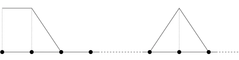
In one dimension we use the more natural notation that the boundary nodes are numbered

(7)

[image:7.612.102.493.32.131.2]

Boundary node

Internal node

Figure 1: Test functions for the recovery ofU via mass conservation in one dimension which

are compatible with strong imposition of Dirichlet boundary conditions.

goals of Dirichlet conditions and mass conservation are easily achieved by taking

f

W1(t, x) = W0(t, x) +W1(t, x) and WNf (t, x) = WN(t, x) +WN+1(t, x), (18)

leaving the remaining Wi(t, x) unaltered. The family of modified piecewise linear test

func-tions is illustrated in Figure 1 and leads to the set of equafunc-tions

Z XN+1(t)

X0(t)

(W0+W1)U dx = Ce1 = C0+C1

Z XN+1(t)

X0(t)

WiU dx = Cie = Ci for i= 2, . . . , N −1

Z XN+1(t)

X0(t)

(WN +WN+1)U dx = CNe +1 = CN +CN+1. (19)

The trial space is based upon the usual piecewise linear basis, with the coefficients of W0

and WN+1 overwritten by the Dirichlet boundary conditions. Adding together equations

(19) shows that this approach retains global mass conservation, albeit with modified local masses that have the same total mass. Importantly, the additional terms make the mass matrix more diagonally dominant.

2.2 Two Dimensions

In two dimensions the test functions can be similarly modified, in such a way that they retain the same support as the original hat functions but with the test functions adjacent to the boundary distributed to interior test functions. The mapping is non-unique and two possible choices will be described here.

i. The first approach is derived by decomposing the mass associated with any test function

corresponding to a boundary node into components obtained by integrating the overlapping

trial functions over each of the neighbouring cells. For example, consider a node, I say, on

(8)

k

J

K

I

3

2

1 j

4

[image:8.612.148.447.15.154.2]

l

Figure 2: Boundary nodes for two-dimensional boundary conditions. The thicker line repre-sents the boundary edges.

2, the mass associated with node I is given by

Z

Ω(t)

WI(t,x)U(t,x)dx =

Z

△1

WI(WIUI+WJUJ +WjUj)dx

+

Z

△2

WI(WIUI+WjUj +WkUk)dx

+

Z

△3

WI(WIUI+WkUk+WKUK)dx. (20)

The upper case subscripts indicate boundary nodes while lower case subscripts signify in-ternal nodes. This is more complicated than the one-dimensional case because many of the boundary nodes have more than one adjacent node to which their contributions can be

trans-ferred. Furthermore, even though the values of U(t,x) on the boundary remain constant

during the time evolution, their contribution to the integral in (20) does not (because the nodal positions in the moving mesh method may change), so they cannot be ignored (this is also true in one dimension).

The boundary cells can clearly be split into two categories, one of which is far simpler to deal with.

• When a triangular cell has two vertices on the boundary and one in the interior, the

full mass of the cell can be transferred to the internal node.

• When a triangular cell has one vertex on the boundary and two in the interior, the

(9)

The resulting split is more clearly illustrated by the annotation of the terms in (20) given by

Z

Ω(t)

WI(t,x)U(t,x)dx =

Z

△1

WI(WIUI+WJUJ +WjUj)dx +

Z

△2

WI(WjUj)dx

| {z }

add to equation j

+

Z

△3

WI(WIUI+WkUk+WKUK)dx +

Z

△2

WI(WkUk)dx

| {z }

add to equation k

+

Z

△2

WI(WIUI)dx

| {z }

split between j and k

. (21)

The right-hand side constants Ci in Equation (11) are calculated from a piecewise linear

representation of the dependent variable, and can therefore be partitioned in the same way as in (21). The test functions indicated by (21), examples of which are provided in Figure 3, are clearly discontinuous, but this has no adverse effects on the computation, since no derivatives are required. Figure 3 also shows that the test functions for nodes which are not adjacent to the boundary remain unchanged.

In algebraic terms, the test function associated with node k in Figure 2 would take the

form

f

Wk = Wk+ WI|△₃+ WK|△₃ +

λ2,k λ2,j+λ2,k

WI|△₂ +

λ4,k λ4,k+λ4,l

WK|△₄ , (22)

in which W|△ indicates the test function restricted to the specified triangular mesh cell, and

the λ are chosen appropriately. Since the support for each of the modified test functions is

the same as that of the corresponding standard linear test function, this will be referred to

as the compact modified approach. Furthermore, this method adds to the diagonal of the

mass matrix, making it more diagonally dominant and potentially easier to invert.

The special case in which zero Dirichlet boundary conditions are applied is considerably

simpler. In this situation, the mass associated with node I, according to the connectivity

shown in Figure 2, is given by

Z

Ω(t)

WI(t,x)U(t,x)dx

=

Z

△1

WIU dx +

Z

△2

WIU dx +

Z

△3

WIU dx

=

Z

△1

WI(WjUj)dx +

Z

△2

WI(WjUj+WkUk)dx +

Z

△3

WI(WkUk)dx

=

Z

Ω(t)

WI(WjUj)dx

| {z }

add to equation j

+

Z

Ω(t)

WI(WkUk)dx

| {z }

add to equation k

. (23)

(10)

[image:10.612.108.499.47.188.2]

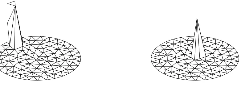
Boundary node Internal node

Figure 3: Representative test functions for the recovery of U via mass conservation in two

dimensions which are compatible with strong imposition of Dirichlet boundary conditions using the “compact” approach.

out for one dimension in (19). The boundary values may then be overwritten with zero

Dirichlet conditions and the internal equations solved for the internal values of U without

losing mass. A similar approach can be followed however many internal nodes are adjacent to

I. (In the special case where node I has no adjacent internal nodes, the boundary condition

U = 0 ensures that node I does not contribute to the overall mass and can therefore be

ignored.) Exactly the same partition can be applied to (12) to obtain (17).

The distribution of the mass indicated by (23) can be achieved using modified test

func-tions of the form (22) in which λ=U. Since

Z

△2

WIWk dΩ =

Z

△2

WIWj dΩ (24)

it is simple to show that

Z

△2

Uk

Uj+UkWIU dΩ = Z

△2

WI(WkUk)dΩ, (25)

with a similar equality for Uj, from which the equivalence of the schemes based on (22) and

(23) follows immediately. In the presence of non-homogeneous Dirichlet boundary conditions, (25) no longer holds, and using a test function of the form (22) in (16) would seem to

require the inversion of a nonlinear system of equations to recover the nodal values of U.

However, this can be easily avoided by lagging the values of U, using the values from the

(11)

[image:11.612.106.500.56.188.2]

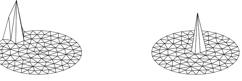
Boundary node Internal node

Figure 4: Representative test functions for the recovery of U via mass conservation in two

dimensions which are compatible with strong imposition of Dirichlet boundary conditions using the “averaged” approach.

ii. The second approach considered here modifies the test functions directly simply by

redistributing the test functions associated with the boundary nodes equally between the

adjacent internal nodes to give, in the case of node k in Figure 2,

f

Wk = Wk+ 1

NIWI+

1

NKWK, (26)

in which NI and NK represent the number of internal nodes connected by the mesh to

boundary nodes I and K, respectively. This scheme will be referred to as the averaged

modified approach. The logic required to implement this form is simpler than for the first, and the resulting system given by (16) is always linear, but the modification is not guaranteed to increase the diagonal dominance of the mass matrix and it can extend the stencil of the scheme, especially in three dimensions (and hence reduce the sparsity of the mass matrix

where a boundary node has more than d internal neighbours, d being the number of space

dimensions).

3 Numerical Experiments

In this section we compare the results obtained from the particular ALE method [1], applied to two different moving boundary problems, in the following cases:

A Dirichlet conditions are imposed weakly and mass is conserved exactly (as in [1]),

B Dirichlet conditions are imposed strongly and mass is conserved exactly using the

modified test functions (as described in the previous section). In two dimensions, the two different forms described in Section 2.2 are used:

(12)

ii the averaged modified approach.

3.1 The Porous Medium Equation

We first present numerical results for a problem of the form (1) which satisfies the boundary condition (4) on its whole boundary. The porous medium equation (PME) takes the form

∂u

∂t = ∇ ·(u n

∇u), (27)

where n > 0 is an integer exponent, on a moving domain R(t) with the Dirichlet boundary

conditionu= 0 on∂R(t). It is well known that solutions exist with finite but time-dependent

support in which mass (the integral of the dependent variable u over the whole domain)

is conserved. In particular, equation (27) admits a family of compact-support similarity

solutions with moving boundaries at which u = 0 (see, for example, [4, 11]). Two of these

solutions are considered here, one with exponentn= 1 (for which the slope of the self-similar

solution normal to the moving boundary is finite) and the other with n = 3 (for which the

slope normal to the boundary is infinite).

It can be shown that in d space dimensions (here d = 1 or 2) a radially symmetric

self-similar solution exists of the form

u(r, t) =

    

1

λd₍_t₎

1− r

r0λ(t)

2n1

|r| ≤r0λ(t)

0 |r|> r0λ(t),

(28)

in which r is the usual radial coordinate, and where

λ(t) =

t t0

1

2+dn

and t0 =

r02n

2(2 +dn). (29)

Symmetry is not assumed in the numerical calculations carried out here, so in one

dimen-sion, for example, the whole of the solution support [−r, r] is modelled. The problem is

parameterised by the initial front positionr0 at timet0, and the position of the moving front

is given by r0λ(t). The test cases are run until timeT =t−t0.

Results are computed for four test cases, two each in one and two space dimensions.

• One dimension, n = 1, r0 = 0.5, t0 = 0.04167 run until T = 10 (when r≈3.11154).

• One dimension, n = 3, r0 = 0.5, t0 = 0.075 run until T = 10 (whenr ≈1.33231).

• Two dimensions, n = 1, r0 = 0.5, t0 = 0.03125 run until T = 0.1 (when r ≈0.71578).

• Two dimensions, n= 3, r0 = 0.5,t0 = 0.046875 run until T = 0.1 (when r≈0.57673).

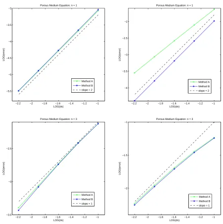
All the results have been obtained on quasi-uniform meshes, for which the representative

(13)

−2.2 −2 −1.8 −1.6 −1.4 −1.2 −1 −5.5

−5 −4.5 −4 −3.5 −3

LOG(dx)

LOG(error)

Porous Medium Equation: n = 1

Method A Method B slope = 2

−2.2 −2 −1.8 −1.6 −1.4 −1.2 −1 −4

−3.5 −3 −2.5 −2

LOG(dx)

LOG(error)

−2.2 −2 −1.8 −1.6 −1.4 −1.2 −1 −3.5

−3 −2.5

LOG(dx)

LOG(error)

−2.2 −2 −1.8 −1.6 −1.4 −1.2 −1 −2

−1.5 −1

LOG(dx)

LOG(error)

[image:13.612.69.520.93.545.2]

Figure 5: Comparison ofL2 _{errors in the solution (left) and the magnitudes of the errors in}

(14)

−2 −1.8 −1.6 −1.4 −1.2 −1 −0.8 −5

−4.5 −4 −3.5 −3

LOG(dx)

LOG(error)

Method A Method Bi Method Bii slope = 2

−2 −1.8 −1.6 −1.4 −1.2 −1 −0.8 −5

−4.5 −4 −3.5 −3

LOG(dx)

LOG(error)

−2 −1.8 −1.6 −1.4 −1.2 −1 −0.8 −2.5

−2 −1.5

LOG(dx)

LOG(error)

−2 −1.8 −1.6 −1.4 −1.2 −1 −0.8 −2.5

−2 −1.5

LOG(dx)

LOG(error)

[image:14.612.72.519.109.547.2]

Figure 6: Comparison ofL2 _{errors in the solution (left) and boundary node positions (right)}

(15)

[image:15.612.109.486.83.190.2]

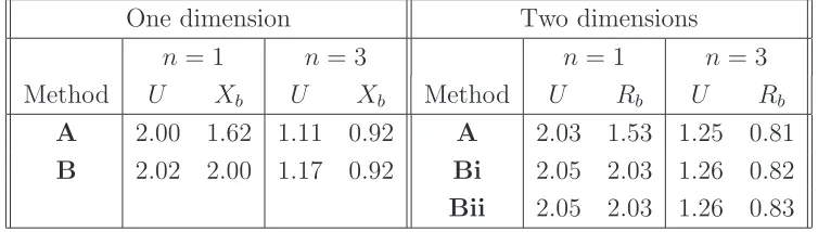
Table 1: Numerical estimates of the orders of accuracy of the scheme for the dependent

variable U and the boundary positions Xb or Rb using each set of boundary conditions,

obtained by comparing errors on the finest pair of meshes used in the experiments.

One dimension Two dimensions

n= 1 n = 3 n= 1 n = 3

Method U Xb U Xb Method U Rb U Rb

A 2.00 1.62 1.11 0.92 A 2.03 1.53 1.25 0.81

B 2.02 2.00 1.17 0.92 Bi 2.05 2.03 1.26 0.82

Bii 2.05 2.03 1.26 0.83

The values of various error measures are shown in Figures 5 and 6, while numerically esti-mated orders of accuracy are given in Table 1.

These results lead to a number of observations.

• The results obtained using methodsBiandBiiin the two-dimensional cases are almost

indistinguishable in terms of speed and accuracy. In the discussion below they will be

considered together and referred to simply as method B.

• There can be significant differences between the errors in approximating the boundary

position in the two methods, even when the errors in the solution approximation are very similar.

• Typically, the method is second order accurate when n= 1 and first order accurate or

slightly better when n= 3, whichever approach is used.

• Overall, the least accurate of the approaches seems to be the one which only imposes

U = 0 weakly (method A). This is most noticeable when considering the error in the

boundary position, where for n = 1 the numerical evidence suggests that the order of

accuracy drops by about 0.5.

• In terms of computational speed, the methods are very similar, though method B is

typically slightly faster, partly because it is inverting a smaller system when recovering the values of the dependent variable, and partly because the adjustments made to the mass matrix tend to improve its conditioning and so accelerate the convergence of the conjugate gradient algorithm used to invert the mass matrix.

• Neither method constrains the dependent variable from becoming negative, but the

nature of the solutions tested has meant that this has only happened when the Dirichlet

boundary condition is enforced weakly (method A). The negative values (when they

(16)

• The solution was initialised with the piecewise linear interpolant of the exact solution values at the nodes of the initial mesh. The same experiments have been run using a constrained best least squares fit to provide the initial values for the dependent

variable. Similar orders of accuracy were seen when using method B, but typically the

least squares fit gave better solutions for n = 3, whilst the exact nodal values were

better for n = 1.

Of the two general approaches, methodB, which allows exact mass conservation and Dirichlet

boundary conditions to be achieved simultaneously, clearly has the better combination of accuracy, robustness, speed and physical realism, when applied in the context of this moving mesh method. Hence this approach is recommended for future use. Since there is little to

distinguish between methodsBiand Biiin terms of speed and accuracy, either would be an

appropriate choice in two-or three-dimensional simulations, although Bii has the attraction

of greater simplicity, even though the modified test functions may have a greater support.

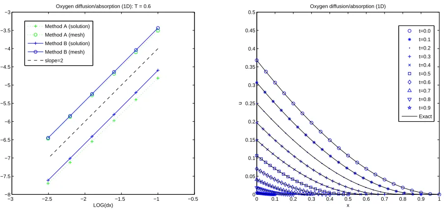
3.2 A Diffusion-Absorption Problem

In addition to examples of the form (1), or for which the total mass is constant in time, we illustrate here that the technique proposed may also be applied to more general problems for which both mass conservation and Dirichlet boundary conditions are still important. This test case represents a moving boundary problem with a source term, described in [5], which models the diffusion of oxygen in an absorbing medium. The equation takes the form

∂u

∂t = ∇

2_u₋₁ _with _u_|

∂Ω(t) =

∂u ∂n _∂

Ω(t)

= 0, (30)

in which ∂Ω(t) represents the moving boundary only. Details of how the moving mesh finite

element approach can be modified to approximate this system can be found in [1]. For the one-dimensional version of this problem an exact solution is known, [5]:

u(x, t) =

(

−x−t+ex+t−₁

x≤1−t

0 x >1−t , (31)

with initial conditions at t0 = 0. In this one-dimensional case an additional boundary

condition is also required at the fixed boundary x= 0, and here the exact value of ux(0, t)

(from (31)) is imposed, as in [1]. Note that it is now the proportion of the total mass

associated with each node which is held constant by the algorithm. The rate of change of mass for this problem is known, and can be used to modify the right-hand side of (11) and (16) appropriately.

(17)

• 1.92 for method A compared with 1.99 for method B for the dependent variable u.

• 1.98 for methodAcompared with 2.00 for methodBfor the moving boundary position

[image:17.612.74.526.168.382.2]

xN+1.

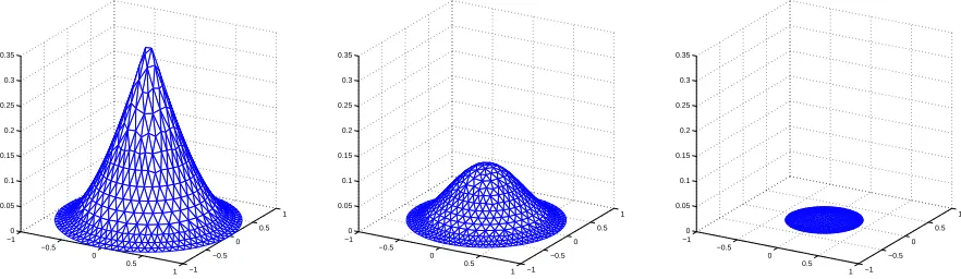
Figure 8 shows the evolution of the corresponding two-dimensional problem (for which no

exact solution is available to the authors) obtained using method Bi. The initial conditions

are given by (31) at t = 0, with x replaced byr, the usual radial coordinate.

−3 −2.5 −2 −1.5 −1 −0.5

−8 −7.5 −7 −6.5 −6 −5.5 −5 −4.5 −4 −3.5 −3

LOG(dx)

LOG(error)

Oxygen diffusion/absorption (1D): T = 0.6

Method A (solution) Method A (mesh) Method B (solution) Method B (mesh) slope=2

0 0.1 0.2 0.3 0.4 0.5 0.6 0.7 0.8 0.9 1 0

0.05 0.1 0.15 0.2 0.25 0.3 0.35 0.4 0.45 0.5

x

u

Oxygen diffusion/absorption (1D)

t=0.0 t=0.1 t=0.2 t=0.3 t=0.4 t=0.5 t=0.6 t=0.7 t=0.8 t=0.9 Exact

Figure 7: Accuracy of the approximate solutions on a sequence of meshes atT = 0.6 (left) and

the evolution of the exact and approximate solutions fromT = 0.0 to T = 0.9 (right). The

solution error shown is an L2 _{approximation while the mesh error is simply the magnitude}

of the error in the boundary position.

4 Discussion

In this paper we have discussed the strong imposition of Dirichlet boundary conditions at the same time as conserving mass in the finite element modelling of moving boundary problems. It has been demonstrated that both constraints can be made to hold simultaneously if the test space is modified in a relatively simple way. In one dimension the modification is immediate, in two dimensions slightly more complicated, but can be extended simply to three dimensions.

(18)

that an approach which imposes both mass conservation and boundary conditions strongly is superior. The improved conditioning of the mass matrix also makes the method more efficient and this approach is recommended. This recommendation includes problems for which the total mass is not constant since, for the problem defined in (30), in which the mass varies in a known manner due to the influence of a source term, the new approach improved the order of accuracy of the approximation.

As described in Section 1, the problem of imposing both strong Dirichlet boundary con-ditions and mass conservation arises for any ALE formulation which correctly captures the motion of the moving boundary (see Equation (4)). In particular, when Dirichlet conditions are imposed in the usual finite element manner, so that equations (7) are solved only for

i= 1, ..., N, mass is not conserved. The technique proposed here, in which the test functions are modified as described in Section 2, may be applied in any such situation. Specifically, if

V(t) is known, and satisfies the discrete form of the boundary condition (4), the right-hand

side of (6) or (7) can be evaluated and used to give the values of (8) at the new time level, as described in [3] for example. Modification of the test functions as illustrated by (22) or (26), can then be applied to allow simultaneous application of boundary conditions and

mass conservation. In the case where λ = U is used in (22) a similar issue arises as when

non-homogeneous Dirichlet boundary conditions are considered, so the nodal values of U

must be lagged in the definition of the test function.

In Section 2.2 the modification was considered in terms of redistributing the mass asso-ciated with each boundary node to internal nodes. Viewed in this context, the particular

moving mesh finite element method used above calculates the constants Ci in Equation (11)

from an initial piecewise linear representation of the dependent variable, so they could be distributed in the manner described by Equation (21). Now, when considering the mesh connectivity shown in Figure 2, the updated values of the quantities on the right-hand side

[image:18.612.74.515.459.587.2]

−1 −0.5 0 0.5 1 −1 −0.5 0 0.5 1 0 0.05 0.1 0.15 0.2 0.25 0.3 0.35 −1 −0.5 0 0.5 1 −1 −0.5 0 0.5 1 0 0.05 0.1 0.15 0.2 0.25 0.3 0.35 −1 −0.5 0 0.5 1 −1 −0.5 0 0.5 1 0 0.05 0.1 0.15 0.2 0.25 0.3 0.35

Figure 8: Approximate solution surfaces at three different times (t = 0.0, 0.05 and 0.1) for

(19)

of (6) can be broken up no further than

Z

Ω(t)

WIf dx =

Z

△1

WIf dx +

Z

△2

WIf dx +

Z

△3

WIf dx. (32)

Here the precise definition of f depends upon the time integration scheme used to solve

(6) to obtain (8) at the new time level, and U is regularised as necessary. As before, the

contributions from triangles 1 and 3 can, in each case, be transferred to the unique internal vertex (as can also be done in one dimension). The contribution from triangle 2 can be split and, for consistency with the process illustrated by Equation (23), should be carried out as

follows (cf.Equation (22)):

Z

△2

WIf dx = fj

fj+fk Z

△2

WIf dx

| {z }

add to equation j

+ fk

fj +fk Z

△2

WIf dx

| {z }

add to equation k

. (33)

The solution U then preserves the integral of f and therefore the total mass.

Interestingly, the simple idea presented in this paper may also be applied in a range of different contexts. For example, it is applicable when mass conservation is required alongside

any specific constraint on the value ofuin equations such as (1), not only constraints on the

boundary of the domain. A similar situation arises in finding a constrained L2 _{best fit to a}

fixed function in any number of space dimensions when, for example, mass conservation is required.

5 Acknowledgements

The authors would like to thank the referee for some very useful suggestions which have

significantly improved the paper, particularly through the inclusion of method Bii. The

authors also thank EPSRC for supporting the research through grant no. EP/D058791/1.

References

[1] M.J.Baines, M.E.Hubbard and P.K.Jimack, A moving mesh finite element algorithm for the adaptive solution of time-dependent partial differential equations with moving

boundaries, Appl. Numer. Math., 54:450–469, 2005.

[2] M.J.Baines, M.E.Hubbard and P.K.Jimack, A moving mesh finite element algorithm

for fluid flow problems with moving boundaries, Int. J. Numer. Methods Fluids,

47(10/11):1077–1083, 2005.

[3] M.J.Baines, M.E.Hubbard, P.K.Jimack and A.C.Jones, Scale-invariant moving finite

elements for nonlinear partial differential equations in two dimensions, Appl. Numer.

(20)

[4] G.I.Barenblatt, Scaling, CUP, 2003.

[5] A.E.Berger, M.Ciment and J.C.W.Rogers, Numerical solution of a diffusion

consump-tion problem with a free boundary, SIAM J. Numer. Anal., 12:646–672, 1975.

[6] C.J.Budd, G.J.Collins, W.Huang and R.D.Russell, Self-similar numerical solutions of

the porous-medium equation using moving mesh methods, Phil. Trans. Roy. Soc.

Lon-don, 357:1047–1077, 1999.

[7] W.Cao, W.Huang and R.D.Russell, A moving mesh method based on the geometric

conservation law, SIAM J. Sci. Comput., 24:118–142, 2002.

[8] W.Huang, Y.Ren and R.D.Russell, Moving mesh methods based on moving mesh partial

differential equations, J. Comput. Phys., 113:279–290, 1994.

[9] R.Li, T.Tang and P.Zhang, A moving mesh finite element algorithm for singular

prob-lems in two and three space dimensions, J. Comput. Phys., 177:365–393, 2002.

[10] J.A.Mackenzie and M.L.Robertson, A moving mesh method for the solution of the

one-dimensional phase-field equations, J. Comput. Phys., 181(2):526–544, 2002.

[11] J.D.Murray, Mathematical Biology: An Introduction (3rd edition), Springer, 2002.

[12] J. Ockendon, S. Howison, A Lacey and A Movchan, Applied Partial Differential Equa-tions (revised edition), Oxford University Press, 2003.

[13] B.V.Wells, M.J.Baines and P.Glaister, Generation of arbitrary Lagrangian-Eulerian (ALE) velocities, based on monitor functions, for the solution of compressible fluid

equations, Int. J. Numer. Methods Fluids,47(10/11):1375–1381, 2005.

[14] P.Wesseling, Computational Fluid Dynamics, Springer, 2000.

[15] P.Zegeling, Moving Grid Techniques, in Handbook of Grid Generation, J.F.Thompson,

B.K.Soni, N.P.Weatherill (Eds.), CRC Press, 37-1 – 37-18, 1999.

A

Derivation of the Nodal Velocities

The mesh velocities for the moving mesh finite element method of [1] are derived by dif-ferentiating the integral in (11) with respect to time. Assuming the existence of a velocity potential, and integrating by parts, this leads to an equation for a piecewise linear

approx-imation, Φ, to the velocity potential which, with zero Dirichlet boundary conditions for U

and FU (for simplicity of this exposition), is

Z

Ω(t)

U(t,x)∇Φ· ∇Wi dx = −

Z

Ω(t)

(21)

The velocity V is obtained by a bestL2 _{fit to} _∇_Φ,

Z

Ω(t)

Wi(t,x)V(t,x)dx =

Z

Ω(t)

Wi(t,x)∇Φdx. (35)

A single time-step of the moving mesh finite element method then consists of the following stages [1].

1. Given a set of mesh nodes with positions Xi solve (11) to obtain the solution values

Ui at the mesh nodes, i = 1, . . . , N +B. The constants Ci are calculated from the

initial solution and mesh. This is the stage where the techniques of this paper may be applied.

2. Use the values of Ui in (34) to obtain the velocity potentials Φi at the mesh nodes

i= 1, . . . , N+B. In order to ensure that (34) has a unique solution, Φ = 0 is fixed at one point in the computational domain, with the remaining equations solved for every other node.

3. Use the values of Φi in (35) to obtain the mesh node velocitiesVi fori= 1, . . . , N+B,

without imposing boundary conditions on V.

These three steps can be thought of as evaluating a function of the form F~(X~) (the arrows

indicate a vector which contains the values stored at all of the nodes of the mesh) which satisfies

d ~X

dt = F~(X~) = V~ . (36)

This system of ordinary differential equations in time can then be integrated using any appropriate method. In [1], a simple forward Euler discretisation was used, but in this paper Heun’s scheme, a second order TVD Runge-Kutta discretisation, is used to ensure that the errors due to approximating the time derivative are negligible compared to those incurred by the spatial discretisation. The qualitative features of the results presented in this paper are not changed by switching to the first order scheme, but the quantitative differences can be assessed using the comparison presented in Figures 9, 10 and 11. It is clear from the figures that the second order scheme is accurate enough to ensure that the errors due to the temporal discretisation are negligible for almost any value of the time-step which avoids mesh tangling. A fourth order Runge-Kutta scheme was also used, but the additional accuracy was unnecessary for this work.

(22)

−6 −5.5 −5 −4.5 −4 −3.5 −3 −2.5 −2 −1.5 −5.5

−5 −4.5 −4 −3.5 −3 −2.5

LOG(dt)

LOG(error)

161 node mesh 81 node mesh 41 node mesh 21 node mesh 11 node mesh

Forward Euler Heun

−6 −5.5 −5 −4.5 −4 −3.5 −3 −2.5 −2 −1.5 −4.5

−4 −3.5 −3 −2.5 −2 −1.5

LOG(dt)

LOG(error)

Forward Euler Heun

−6 −5.5 −5 −4.5 −4 −3.5 −3 −2.5 −2 −1.5 −3.5

−3 −2.5 −2

LOG(dt)

LOG(error)

Forward Euler Heun

−6 −5.5 −5 −4.5 −4 −3.5 −3 −2.5 −2 −1.5 −2.5

−2 −1.5 −1

LOG(dt)

LOG(error)

[image:22.612.72.520.79.525.2]

Forward Euler Heun

Figure 9: Comparison of L2 _{errors in the solution (left) and the magnitudes of the errors}

(23)

−5.5 −5 −4.5 −4 −3.5 −3 −2.5 −2 −5

−4.5 −4 −3.5 −3 −2.5

LOG(dt)

LOG(error)

8321 node mesh 2113 node mesh 545 node mesh 145 node mesh

Forward Euler Heun

−5.5 −5 −4.5 −4 −3.5 −3 −2.5 −2 −5

−4.5 −4 −3.5 −3 −2.5

LOG(dt)

LOG(error)

Forward Euler Heun

−5.5 −5 −4.5 −4 −3.5 −3 −2.5 −2 −3

−2.5 −2 −1.5 −1

LOG(dt)

LOG(error)

Forward Euler Heun

−5.5 −5 −4.5 −4 −3.5 −3 −2.5 −2 −2.5

−2

LOG(dt)

LOG(error)

[image:23.612.72.520.87.536.2]

Forward Euler Heun

Figure 10: Comparison of L2 _{errors in the solution (left) and boundary node positions}

(24)

−7 −6.5 −6 −5.5 −5 −4.5 −4 −3.5 −3 −2.5 −8

−7.5 −7 −6.5 −6 −5.5 −5 −4.5 −4

LOG(dt)

LOG(error)

Diffusion−Absorption Problem

321 node mesh 161 node mesh 81 node mesh 41 node mesh 21 node mesh 11 node mesh

Forward Euler Heun

−7 −6.5 −6 −5.5 −5 −4.5 −4 −3.5 −3 −2.5 −7

−6.5 −6 −5.5 −5 −4.5 −4 −3.5 −3

LOG(dt)

LOG(error)

Diffusion−Absorption Problem

321 node mesh 161 node mesh 81 node mesh 41 node mesh 21 node mesh 11 node mesh

[image:24.612.78.516.196.411.2]

Forward Euler Heun

Figure 11: Comparison of L2 _{errors in the solution (left) and the magnitudes of the errors}