This is a repository copy of
Nonlinear theory of resonant slow waves in anisotropic and
dispersive plasmas
.
White Rose Research Online URL for this paper:
http://eprints.whiterose.ac.uk/10486/
Article:
Clack, C.T.C. and Ballai, I. (2008) Nonlinear theory of resonant slow waves in anisotropic
and dispersive plasmas. Physics of Plasmas, 15 (8). Art. No. 082310. ISSN 1089-7674
https://doi.org/10.1063/1.2970947
eprints@whiterose.ac.uk https://eprints.whiterose.ac.uk/
Reuse
Unless indicated otherwise, fulltext items are protected by copyright with all rights reserved. The copyright exception in section 29 of the Copyright, Designs and Patents Act 1988 allows the making of a single copy solely for the purpose of non-commercial research or private study within the limits of fair dealing. The publisher or other rights-holder may allow further reproduction and re-use of this version - refer to the White Rose Research Online record for this item. Where records identify the publisher as the copyright holder, users can verify any specific terms of use on the publisher’s website.
Takedown
If you consider content in White Rose Research Online to be in breach of UK law, please notify us by
arXiv:0903.0948v1 [astro-ph.SR] 5 Mar 2009
and dispersive plasmas
Christopher TM Clack and Istvan Ballai
Solar Physics and Space Plasma Research Centre (SP2 RC),
Department of Applied Mathematics, University of Sheffield, Hicks Building, Hounsfield Road, Sheffield, S3 7RH, U.K.
The nonlinear theory of driven magnetohydrodynamics (MHD) waves in strongly anisotropic and dispersive plasmas, developed for slow resonance by Clack & Ballai [Phys. Plasmas 15(8), 2310 (2008)] and Alfv´en resonance by Clacket al. [A&A494, 317 (2009)], is used to study the weakly nonlinear interaction of fast magnetoacoustic (FMA) waves in a one-dimensional planar plasma. The magnetic configuration consists of an inhomogeneous magnetic slab sandwiched between two regions of semi-infinite homogeneous magnetic plasmas. Laterally driven FMA waves penetrate the inhomogeneous slab interacting with the localized slow or Alfv´en dissipative layer and are partly reflected, dissipated and transmitted by this region. The nonlinearity parameter defined by Clack & Ballai (2008) is assumed to be small and a regular perturbation method is used to obtain analytical solutions in the slow dissipative layer. The effect of dispersion in the slow dissipative layer is to further decrease the coefficient of energy absorption, compared to its standard weakly nonlinear counterpart, and the generation of higher harmonics in the outgoing wave in addition to the fun-damental one. The absorption of external drivers at the Alfv´en resonance is described within the linear MHD with great accuracy.
PACS numbers: 52.25.Fi; 52.30.Cv; 52.35.-g; 52.35.Bj; 52.35.Mw
I. INTRODUCTION
The problem of interacting fast magnetoacoustic (FMA) waves with different magnetic structures is not only important in the context of astrophysics and solar physics, but also in laboratory plasma devices. Space and laboratory plasmas are highly non-uniform and dy-namical systems and as a consequence they are a natural medium for magnetohydrodynamic (MHD) waves. When the magnetic plasma configuration is inhomogeneous in the transversal direction relative to the ambient magnetic field a phenomenon, known as resonant absorption, oc-curs (see, e.g., Appert et al. [1] and Ionson [2]). Some of the wave energy can be converted into heat in a thin layer which embraces the ideal resonant magnetic surface when dissipative processes are taken into account.
In the context of solar physics, the resonant coupling of waves was first suggested by Ionson(author?) [3] as a possible mechanism for heating coronal loops. Shortly after, several studies on the efficiency of resonant ab-sorption in the complicated process of coronal heating were published by, e.g., Ionson(author?) [2],
Kupe-rus et al.(author?) [4], Davila(author?) [5] and
Holl-weg(author?) [6]. The same principle was used to ex-plain the observed loss of power of acoustic oscillations in the vicinity of sunspots by, e.g., Hollweg(author?)
[7], Lou(author?) [8], Sakurai et al.(author?) [9], Goossens and Poedts(author?)[10], Goossens and Holl-weg(author?) [11] and Stenuit et al.(author?) [12]. All these studies dealt with the Alfv´en resonant posi-tion. Although happening at lower frequencies, slow res-onance is also important as shown in a study by Kep-pens(author?) [13] where he investigated the interac-tion of sound waves with hot evacuated magnetic fibrils.
Most of the analytical studies of resonant absorption were based on the linear theory due to its relative simplicity.
A new approach to the problem of resonant absorp-tion in the context of high Reynolds number plasmas was given by Rudermanet al.(author?) [14] who developed a nonlinear theory of resonant absorption for slow waves in isotropic plasmas. They pointed out that nonlinearity has to be taken into account under typical solar condi-tions near resonance. The theory of nonlinear resonant slow waves was extended to strongly anisotropic plasmas in Ballaiet al.(author?)[15] to describe conditions typ-ical for the solar chromosphere and corona. Over the next few years there was an enormous amount of effort put into studying resonant absorption, including the in-vestigation of the effect of equilibria flows at the slow res-onance (see, e.g., Ballai and Erd´elyi [16]), the absorption of sound waves at the slow dissipative layers in isotropic and anisotropic plasmas (see, e.g., Rudermanet al. [17] and Ballai et al. [18]) and the effect of an equilibrium flow on the absorption of sound and FMA waves due to the coupling in the slow continua (see, e.g., Erd´elyi and Ballai [19] and Erd´elyiet al. [20]). In a recent paper, Clack and Ballai(author?)[21] showed that in strongly anisotropic and dispersive plasmas the dispersion, dissi-pation and nonlinearity are all of the same order inside the dissipative layer.
showed that the largest nonlinear and dispersive terms cancel out - leaving only small corrections to linear the-ory.
Many studies of resonant absorption considered only the sound (or slow) and Alfv´en waves as excellent candi-dates for coronal heating. Alfv´en waves can only carry energy along the magnetic field lines and slow waves are only able to carry 1−2% of energy under coronal (low plasma-β) conditions. However, FMA waves might have an important role in explaining the coronal temperatures, as has been shown by, e.g., ˘Cade˘z et al.(author?) [23] and Cs´ıket al.(author?)[24].
The aim of the present paper is to study the nonlinear (linear) resonant interaction of externally driven FMA waves with the slow (Alfv´en) dissipative layer in strongly anisotropic and dispersive static plasmas. The governing equations and jump conditions derived earlier by Clack and Ballai(author?)[21] and Clacket al.(author?)[22] will be used to study the efficiency of absorption at the slow and Alfv´en resonance. The paper is organized as follows. In the next section we introduce the governing equations, the equilibrium state and the fundamental as-sumptions which allow analytical progress. In Sec. III we find the solutions describing the waves outside the dissipative layers. Section IV is devoted to the nonlinear solution inside the slow dissipative layer. In Sec. V we derive the solution inside the Alfv´en dissipative layer. In Sec. VI we will calculate the absorption coefficient in the case of slow/Alfv´en resonance. Finally, in Sec. VII we summarize our results and draw our conclusions.
II. GOVERNING EQUATIONS AND ASSUMPTIONS
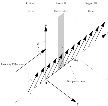
The dynamics and absorption of the waves will be stud-ied in a Cartesian coordinate system. The equilibrium state is shown in Figure 1. The configuration consists of an inhomogeneous magnetized plasma 0 < x < x0 (Region II) sandwiched between two semi-infinite homo-geneous magnetized plasmasx <0 andx > x0 (Regions I and III, respectively). We have chosen this model to ob-tain analytical results. Our intention is to have a model which gives us the trend in the absorption of an inci-dent wave on a magnetic structure. It is obvious that real magnetic structures are more complicated (and far from being fully understood), however, the magnetic field has been simplified to be unidirectional in order to make the model more transparent, such that the role of the dispersion at the resonance and the change in the ab-sorption can be investigated more fully, and compared to previous studies. We took inspiration for this model from seminal studies such as Rudermanet al.(author?)
[17], Ballaiet al.(author?)[18], Erd´elyi(author?)[20], Roberts(author?) [25], Edwin and Roberts(author?)
[26] and Ruderman(author?)[27].
The equilibrium density and pressure are denoted by
ρ and p. The equilibrium magnetic field, B, is
unidi-y z
x
x0
0
α
Incoming FMA wave
φ
Region I Region II Region III
Be, ρe B0(x), ρ0(x) Bi, ρi
[image:3.595.332.543.48.254.2]Dissipative layer
FIG. 1: Illustration of the equilibrium state. Regions I (x <0) and III (x > 0) contain a homogeneous magnetized plasma
and Region II (0< x < x0) an inhomogeneous magnetized
plasma. The shaded strip shows the dissipative layer embrac-ing the ideal resonant positionxc.
rectional and lies in the yz-plane. In what follows the subscripts “e”, “0” and “i” denote the equilibrium quan-tities in the three regions (Regions I, II, III, respectively). It is convenient to introduce the angle,α, between thez -axis and the direction of the equilibrium magnetic field, so that the components of the equilibrium magnetic field are; By = BsinαandBz = Bcosα. All equilibrium
quantities are continuous at the boundaries of Region II, so they satisfy the equation of total pressure balance. It follows from the equation of total pressure that the den-sity ratio between Regions I and III satisfy the relation
ρi
ρe
=2c 2
Se+γv2Ae
2c2
Si+γv2Ai
, (1)
where the squares of the Alfv´en and sound speed arev2
A=
B2
0/µ0ρ0 and cS2 = γp0/ρ0. Where µ0 is the magnetic permeability of free space andγis the adiabatic constant. Replace the subscript “0” with “e” for Region I and “i” for Region III. We consider a hot magnetized plasma such thatc2
Si> c2Se, andv2Ai> vAe2 .
The objective of the present paper is to study (i) the combined effect of nonlinearity and dispersion on the in-teraction of incomingfast waveswithslow dissipative lay-ers and (ii) the interaction of incomingfast waves with
Alfv´en dissipative layers. We, therefore, have two
dif-ferent criteria. For interaction of FMA waves with the slow dissipative layer we assume that the frequency of the incoming fast wave is within the slow continuum of the inhomogeneous plasma, so that there is a slow resonant position at x = xc in Region II. Interactions with the
is an Alfv´en resonant point atx=xa in Region II. This
leads to the inequality,cT e< ω/k < cT i, at the slow
reso-nance. Where the square of the cusp speed,c2
T, is defined
by c2
T = c2SvA2/(c2S +v2A). We also have the inequality,
vAe< ω/k < vAi, for Alfv´en resonance. Hereωis the
fre-quency of the incoming fast wave andk= (k2
x+kz2)1/2 is
the wave number. Even though, in principle, when a slow resonance occurs in this manner an Alfv´en resonance is also present we ignore the Alfv´en resonance that occurs alongside the slow resonance as this would complicate the analysis and obscure the results associated with the slow resonance. We study the Alfv´en resonance separately to the slow resonance. We note that the Alfv´en resonance would, in simple terms, act to restrict the energy avail-able at the slow resonance. We intend to address the issue of coupled resonances in our next paper, where we will show that the governing equations derived here remain the same (meaning the work here is valid), however, the interaction of the waves between the resonant positions changes the absorption of wave energy.
In an attempt to remove other effects from the analysis we consider the incoming fast wave to be entirely in the
xz-plane, i.e. ky = 0. Rudermanet al.(author?) [17]
suggests aligning the equilibrium magnetic field with the
z-axis, to remove the Alfv´en resonance (if we consider planar waves) from the analysis for slow resonance, how-ever, this is not possible nor necessary here. The disper-sion is dependent on the angle between the equilibrium magnetic field and thez-axis (α), hence ifα= 0 the dis-persion effects disappear, and we recover the governing equation studied by Ballaiet al.(author?) [18].
The inequalities above guarantee that the slow and Alfv´en resonances appears in Region II when studying in the upper chromosphere and the solar corona, re-spectively. The resonant positions, therefore, are de-fined mathematically as: ωc = kcT(xc) cosα and ωa =
kvA(xa) cosα. The position of the resonant points also
provides us with some information about the plasma con-dition. First, in conjunction with Eq. (1) we obtain that
ρi
ρe
= 2c 2
Se+γvAe2
2c2
Si+γvAi2
<1. (2)
Hence, the plasma in region III is more rarefied than in Region I. Secondly, it follows that cT e < cT i and the
plasma in Region III is hotter than the plasma in Region I.
The dispersion relation for the impinging propagating fast waves takes the form
ω2
k2 =
1 2
v2
A+c2S
+h v2
A+c2S
2 −4v2
Ac2Scos2φ
i1/2
,
(3) whereφis the angle between the direction of propagation and the background magnetic field within the xz-plane and k = kxex+kzez. For the sake of simplicity, we
denoteκeas the ratiokx/kz. Since the equilibrium
mag-netic field in thexz-plane is aligned with thez-axis, the
dispersion relation (3) becomes
ω2
k2 =
1 2
(
v2A+c2S
+
vA2 +c2S
2 −4 v
2
Ac2S
1 +κ2
e 1/2)
,
(4) where 1 +κ2
e= 1/cos2φ.
We assume the plasma isstrongly magnetized in the three regions, such that the conditionsωi(e)τi(e)≫1 are satisfied, here ωi(e) is the ion (electron) gyrofrequency and τi(e) is the ion (electron) collision time. Due to the strong magnetic field, transport processes are derived from Braginskii’s stress tensor (see, e.g., Braginskii[28]; Ruderman et al.[29]). As we deal with two separate waves (slow and Alfv´en), we will need to choose the particular dissipative process which is most efficient for these waves. For slow waves, it is a good approximation to retain only the first term of Braginksii’s expression for viscosity, namely compressional viscosity(author?)
[30]. In addition, in the solar upper atmosphere slow waves are sensitive to thermal conduction. In a strongly magnetized plasma, the thermal conductivity parallel to the magnetic field lines dwarfs the perpendicular com-ponent, hence the heat flux can be approximated by the parallel component only(author?) [31]. On the other hand, since Alfv´en waves are transversal and incompress-ible they are affected by the second and third compo-nents of Braginskii’s stress tensor, called shear viscos-ity(author?) [22]. Finally, Alfv´en waves are efficiently damped by finite electrical conductivity, which becomes anisotropic under coronal conditions. The parallel and perpendicular components, however, only differ by a fac-tor of 2, so we will only consider one of them without loss of generality. All other transport mechanisms can be neglected. For further details, please refer to, for ex-ample, Clacket al.(author?)[22], Braginskii(author?)
[28], Rudermanet al.(author?)[29], Hollweg(author?)
[30], Priest(author?) [31] and Porter et al.(author?)
[32].
The dynamics of nonlinear resonant MHD waves in anisotropic and dispersive plasmas was studied by Clack and Ballai(author?) [21] and Clack et al.(author?)
[22]. They derived the governing equations and con-nection formulae necessary to study resonant absorp-tion in slow/Alfv´en dissipative layers. We recall the key steps and necessary results found by Clack and Bal-lai(author?) [21] and Clacket al.(author?) [22].
The efficiency of dissipation, when studying slow dissi-pative layers, in an anisotropic plasma is given by the (compressional) viscous Reynolds number (Re(c)) and
the Pechlet number (Pe), combining to define the
to-tal Reynolds number: R−1
c =R−e(1c)+Pe−1, where Re(c) and Pe are defined by Re(c) = vchlchρ0c/η¯0 and Pe =
vchlchρ0cR/e κ¯k. Here vch is the characteristic velocity
(e.g. the slow magnetoacoustic velocity atx= xc), lch
is the characteristic length,ρ0c =ρ0(xc),Re denotes the
gas constant and κk is the coefficient of thermal
The efficiency of dissipation, when studying Alfv´en dis-sipative layers, in an anisotropic plasma is measured in a slightly different way. Now dissipative processes are described by the (shear) viscous Reynolds number (Re)
and the magnetic Reynolds number (Rm), combining to
define the total Reynolds number: R−1
a = R−e1+R−m1,
where Re =vchlchρ0a/η¯1 and Rm =vchlch/η¯. Here vch
is the characteristic velocity (e.g. the Alfv´en velocity at x = xa), lch is the characteristic length, η1 is the coefficient of shear viscosity andηis the coefficient of fi-nite electrical resistivity. Originally, these total Reynolds numbers were introduced based on intuition, simplicity and linear theory (see, e.g., Sakuraiet al. [9], Goossens
et al. [34] and Goossens and Ruderman [35]). However,
it turned out that using these definitions thestrength of dissipation is the same order of magnitude as the inverse of the total Reynolds numbers. Under chromospheric and coronal conditionsR ≫1 which means that dissipation is only important inside the dissipative layer. Far away from the dissipative layer amplitudes are small, therefore we can use the linear ideal MHD equations to describe the plasma motions far from the resonant position. These equations can be reduced to a system of coupled first or-der PDE’s for the total pressure perturbation,P, and the normal component of the velocity,u,
∂u ∂x = V F ∂P ∂θ, ∂P ∂x =
ρ0A
V ∂u
∂θ. (5)
Here
F = ρ0AC
V4−V2(v2
A+c2S) +vA2c2Scos2α
,
C= v2A+c2S
V2−c2Tcos2α
,
A=V2−vA2cos2α. (6)
The system (5) describes the wave motion far from the ideal resonant position. The singularities in the coeffi-cients A and C give the conditions of Alfv´en and slow resonance. All perturbations depend on the combination
θ=z−V t, whereV =ω/k is the phase speed.
Inside the thin dissipative layers (where the dynamics is described by the nonlinear and dissipative MHD equa-tions) embracing the ideal resonant surfaces (x=xc,x=
xa) we must use the governing equations derived by Clack
and Ballai(author?)[21] and Clacket al.(author?)[22]. The characteristic thickness of the slow dissipative layer,
δc, is
δc=
V3kλ
|∆c|(c2Sc+v2Ac).
(7)
Herek= 2π/LwithLthe wavelength, the subscript “c” indicates that the quantity has been calculated at the slow resonant position. The quantityλis defined by
λ=η0 2v
2
Ac+ 3c
2
Sc
2
3ρ0cv
2
Acc
2
Sc
+(γ−1) 2κ
k v2Ac+c
2
Sc
γρ0cRce
2
Sc
, (8)
and ∆cis simply the gradient of the cusp speed given by
∆c = − dc2T/dx
ccos
2α. Clack and Ballai(author?) [21] showed that nonlinearity and dispersion are impor-tant in the slow dissipative layer if the nonlinearity pa-rameter is greater than unity, N2 = ǫR2
c & 1, where ǫ
is the dimensionless wave amplitude far from the dissi-pative layer. The concept of nonlinear parameters was introduced by Ruderman et al.(author?) [14] for slow waves and Clacket al.(author?) [22] for Alfv´en waves. The two parameters are different not only in their form but also in the values the Reynolds numbers take. In the case of slow waves (damped by compressional viscosity, i.e. the first term in the Braginskii’s viscosity tensor) the Reynolds number that corresponds to a characteris-tic length of 200Mm, a speed of 200kms−1, a density of 10−13kgm−3 and a compressional viscosity coefficient of 5×10⁻²kgm−1s−1 is about 80. Alfv´en waves are effi-ciently damped by shear viscosity which is given by the second and third coefficients of the Bragisnkii’s tensor (here denoted cumulatively asη1). Sinceη1=η0/(ωiτi)2
and under coronal conditionsωiτi is of the order of 105,
we obtain that the coefficient of shear viscosity is about 10 orders of magnitude smaller than the coefficient of compressional viscosity. Now, using the characteristic speed of 1000kms−1, the Reynolds number used in cal-culating the nonlinear parameter in the case of Alfv´en nonlinearity is 4×10¹². The nonlinearity parameter for resonant Alfv´en waves is ǫR2/3 ≪ 1. However, it was shown by Clacket al.(author?) [22] that the waves in this situation remain linear anyway. In the present pa-per, therefore, we do not need the nonlinearity parameter for resonant Alfv´en waves. The characteristic thickness of the Alfv´en dissipative layer,δa, is
δa=
V
k|∆a|
¯
η+ η¯1
ρ0a
1/3
, (9)
with ∆a being the gradient of the Alfv´en speed given by
∆a=− dvA2/dx
acos
2α.
The governing equation inside the slow dissipative layer is(author?)[21]
σc∂qc
∂θ + Λqc
∂qc
∂θ −k
−1∂2qc
∂θ2
−Ψ∂qc
∂σ
∂qc
∂θ =−
kV4
ρ0cv
2
Ac|∆c|
dPe
dθ, (10)
where
σc =
x−xc
δc
, (11)
Λ =R2v
4
Ac|∆|
(γ+ 1)v2
Ac+ 3c
2
Sc
kV8 , (12)
Ψ =R2χ|∆|
2c2
Scv
2
Ac(v
2
Ac+c
2
Sc) sinα
kV13 , (13)
χ=ηωeτe. (14)
term describes the nonlinearity of waves, the third term stands for the dissipative effects while the last term on the left-hand side describes the nonlinear dispersive ef-fects generated after taking into account Hall currents by Clack and Ballai(author?)[21]. The term on the right-hand side can be considered as a driver. We also note thatqc(σc, θ) is the dimensionless component of velocity
parallel to the equilibrium magnetic field andχ=ηωeτe
is the coefficient of Hall conduction(author?)[21]. The governing equation inside the Alfv´en dissipative layer is(author?)[22]
σa∂qa
∂θ −k
∂2q
a
∂σ2
a
= ksinα
ρ0a|∆a|
dPe
dθ, (15)
withσa = (x−xa)/δa. Hereqa(σa, θ) is the dimensionless
component of velocity perpendicular to the equilibrium magnetic field. We should point out here that although nonlinearity and dispersion have been considered when deriving the dynamics of the Alfv´en resonance, the gov-erning equation remains linear regardless of the degree of nonlinearity (for details see Clacket al. [22]).
When studying resonant MHD waves, we are generally not interested in the solution inside the dissipative layer and can consider the dissipative layer as a surface of dis-continuity. Instead, we solve the system (5) and match the solutions at the boundaries of the discontinuity using connection formulae. These connection formulae deter-mine the jumps inuandP across the dissipative layer. In the context of solar plasmas, they were first introduced by Sakuraiet al.(author?) [9]. It was shown by Clack and Ballai(author?)[21] (in complete agreement with Rud-erman et al.(author?) [14] and Ballai et al.(author?)
[15]) that the first connection formula is [P] = 0, where the square brackets denote the jump across the dissipa-tive layer. It can also be shown, in a similar manner, that the same jump condition exists for the Alfv´en resonance. The second connection formula for slow resonance can only be written in implicit form, i.e.
[uc] =−
V
kcos2αP
Z ∞
−∞
∂qc
∂θ dσ, (16)
where we use the Cauchy principal value of the integral because the integral is divergent at infinity. As a result we must solve Eqs. (5) and (10) along with the boundary conditions, [P] = 0 and Eq. (16). In an attempt to fol-low the same procedure utilized for finding solutions at the slow resonance we can write the jump in the normal component of velocity for the Alfv´en resonance in an im-plicit form. For the sake of brevity, we do not show the derivation here, but it follows the procedure to find the jump in the normal component of velocity completed by Clack and Ballai(author?)[21]. This jump is given by
[ua] =
V sinα
k P
Z ∞
−∞
∂qa
∂θ dσ. (17)
Finally, we should note some critical assumption we make to allow analytical progress. From the very begin-ning we must assume that the nonlinearity parameter is
small so that regular perturbation theory can be applied at the slow resonance. We also assume that the inho-mogeneous region is thin in comparison with the wave-length of the impinging wave, i.e. kx0 ≪ 1. Ruder-man(author?)[27] investigated the absorption of sound waves at the slow dissipative layer in the limit of strong nonlinearity. In his analysis nonlinearity dominated dis-sipation in the resonant layer which embraces the dis-sipative layer. He concluded that nonlinearity decreases absorption in the long wavelength approximation, but in-creases it at intermediate values ofkx0, however, the in-crease is never more than 20%. To the best of our knowl-edge, at present, we cannot solve the governing equation (10) in the limit of strong nonlinearity due to the nonlin-ear dispersive term, therefore we restrict our analysis to the weak nonlinear limit. We mention that no such as-sumptions are needed for studying the Alfv´en dissipative layer since the governing equation (15) is linear.
III. SOLUTIONS OUTSIDE THE DISSIPATIVE LAYERS
In what follows we derive a solution for the system (5) in Regions I, II and III. In Region II we only find the solution outside the dissipative layers. Section IV is devoted to finding a solution to Eq. (10) inside the slow dissipative layer and Section V is used to find a solution to Eq. (15) inside the Alfv´en dissipative layer. Outside the dissipative layers, the solutions take identical forms.
A. Region I
The solution of Eq. (5) in Region I is given in the form of an incoming and outgoing fast wave of the form
P=ǫ{pecos [k(θ+κex)] +Acos [k(θ−κex)]}, (18)
u=ǫκeV{pecos [k(θ+κex)]−Acos [k(θ−κex)]}
ρe(V2−v2Aecos2α)
,
(19)
B. Region II
In Region II, the equation for the total pressure,P, is obtained by eliminatingufrom the system (5),
F ∂
∂x
1
ρ0(V2−vA2cos2α)
∂P ∂x
=∂ 2P
∂θ2. (20)
Since we have assumedkx0 ≪1, the ratio of the right-hand side and the left-right-hand side is of the order ofk2x20. It follows that
∂P
∂x =ρ0 V
2−v2
Acos2α
f(θ) +O(k2x2
0), (21) where the function f(θ) is determined by the second equation of (5) and the boundary conditions atx = 0. Equation (21) yields
P =Pe(θ) +f(θ)
Z x
0
ρ0
V2−vA2cos2α
dx+O(k2x2
0). (22) The function Pe(θ) has to be determined by the bound-ary conditions at x= 0. It can be shown that, because [P] = 0, the functionsf(θ) and Pe(θ) take the same val-ues throughout Region II. Noting that the second term in Eq. (22) is of the order ofkx0 we can expressP in a simplified form
P =Pe(θ) + (kx0)P′(x, θ) +O(k2x2
0). (23)
C. Region III
To derive the governing equation for Region III we eliminate the normal component of the velocity from the system (5) to arrive at
∂2P
∂x2 +κ
2
i
∂2P
∂θ2 = 0, (24)
whereκ2
i is defined as
κ2i =−
V4−V2 c2
Si+vAi2
+c2
SivAi2 cos2α
(c2
Si+vAi2 ) (V2−c2T icos2α)
. (25)
Since, for slow dissipative layers,V < cT icosα, it follows
that κ2
i > 0. It also follows that for Alfv´en dissipative
layersκ2
i >0 because V > cT icosα > vAecosα.
There-fore, Eq. (24) is an elliptical differential equation and the wave motion is evanescent in Region III. In reality, there could be wave leakage. The existence of wave leak-age depends on the profile of the slow and Alfv´en speeds in the inhomogeneous region (Region II). For simplicity, we have assumed that the slow and Alfv´en resonances take place at a single location (obviously different for the two resonances), which means the profiles of the slow and Alfv´en speeds are monotonically increasing inside Region II. Should we have a more complex model, the possibility of wave leakage would need to be taken into account.
IV. WEAK NONLINEAR SOLUTION INSIDE THE SLOW DISSIPATIVE LAYER
Since we are not able to solve the governing equation (10) inside the slow dissipative layer analytically, we con-sider the limit of weak nonlinearity (N2 ≪ 1). In ac-cordance with this assumption we rewrite the governing equation (10) and the jump condition (16) as
σ∂qc
∂θ +ǫ
−1ζ
Λ Ψ
qc∂qc
∂θ −ǫ
−1ζ∂qc
∂σ
∂qc
∂θ
−k−1∂
2q
c
∂θ2 =−
V4
ρ0cvAc4 |∆c|x0
dPc
dθ , (26)
[uc] =− V x0
cos2αP
Z ∞
−∞
∂qc
∂θ dσ, (27)
where
qc=
qc
kx0
, ζ=kx0D
2
dΨ
R4 , D
2
d=ǫR4=R2N2. (28)
Note thatζ is of the order ofǫR2, the ratio (Λ/Ψ) is of the order of unity andqc is of the order ofǫ. In what
follows we drop the bar notation and for the rest of this section we drop the subscript “c” on the dimensionless variableq.
We proceed by using a regular perturbation method and look for solutions in the form
f =ǫ
∞
X
n=1
ζn−1fn, (29)
wheref represents any of the quantitiesP,uandq.
A. First order approximation
In the first order approximation, from Eq. (26), we obtain
σ∂q1
∂θ −k
−1∂2q1
∂θ2 =−
V4
ρ0cvAc4 |∆|x0
dP1c
dθ . (30)
Since the total pressure,P, is continuous throughout the dissipative layerand is periodical with respect to θ, we look for a solution in the formg1=ℜ(ˆg1eikθ), whereg1 representsP1,u1andq1 andℜindicates the real part of a quantity.
In Region I the solutions for the pressure and velocity exactly recover the results found in linear theory, i.e.
ˆ
P1=peeikκex+A1e−ikκex, (31)
ˆ
u1=
κeV peeikκex−A1e−ikκex
ρe(V2−v2Aecos2α)
, (32)
whereA1 (and subsequent values ofAi) is the amplitude
side of ˆP1 and ˆu1 represent the incoming wave, while the second terms are the outgoing (reflected) wave. The continuity of the total pressure perturbation at x = 0 and x=x0 in combination with Eq. (23) yields ˆP1, in Region II, as
ˆ
P1=pe+A1+ (kx0)ˆh1, (33)
where ˆhn = ˆhn(x) = ˆPn′(x)−Pˆn′(0), n ≥1. The
so-lution in Region III is obtained by using Eqs. (5), (24) and (33) with the continuity conditions atx=x0. The solution takes the form
ˆ
P1=
n
pe+A1+ (kx0)ˆh1
o
e−kκi(x−x0)
, (34)
ˆ
u1=
iκiV
n
pe+A1+ (kx0)ˆh1
o
ρi(V2−vAi2 cos2α)
e−kκi(x−x0)
. (35)
Utilizing the fact that ˆu1 is continuous at x = 0 and
x= x0, and employing Eqs. (5) and (33) we find that the jump in the normal component of velocity across the dissipative layer is
[ˆu1] = iκiV(pe+A1)
ρi(V2−vAi2 cos2α)
− κeV(pe−A1)
ρe(V2−v2Aecos2α)
−ikV (pe+A1)P Z x0
0
F−1(x)dx
−ikV(kx0)P Z x0
0 ˆ
h1(x)
F(x) dx, (36)
where the expression ofF(x) is given by Eq. (6). Solving Eq. (30) reveals ˆq1to be
ˆ
q1=−V
4(p
e+A1){1 +O(kx0)}
ρ0cv2Ac|∆|x0(σ−i)
. (37)
Substitution of this result into Eq. (27) leads to another definition of the jump in the normal component of veloc-ity across the dissipative layer, namely,
[ˆu1] = −πkV 5(p
e+A1){1 +O(kx0)}
ρ0cv4Ac|∆|cos2α
. (38)
Comparing Eqs. (36) and (38) we obtain that
A1=−peτ−µ+iυ
τ+µ+iυ +O(k
2x2
0), (39) where
τ= πkV
5
ρ0cv4Ac|∆|cos2α
, µ= κeV
ρe(V2−v2Aecos2α)
υ= κiV
ρi(V2−vAi2 cos2α)
−kVP Z x0
0
F−1(x)dx. (40)
When deriving Eq. (39) we have employed the estimate thatkPRx0
0 ˆhn(x)/F(x)dx=O(kx0). The quantityA1 is a complex value. This means that the outgoing (re-flected) wave has a phase alteration compared with the
incoming wave. Thetrue amplitudeof the outgoing wave is given byAf1= (A21(r)+A21(im))1/2(where the subscripts “r” and “im” mean the real and imaginary parts, respec-tively). The Fourier analysis allowsA1to be complex. In general, a complex value ofAnmeans the true amplitude
of the outgoing harmonic is defined as above and a phase of the outgoing wave is shifted by tan−1(A2
n(im)/A
2
n(r)). This definition ofAn applies to all subsequent orders of
approximation.
In Rudermanet al. [17] and Ballaiet al. [18] a similar procedure was carried out. Our results are similar with theirs if we considerBe= 0 andα= 0. This conclusion
is not surprising because the first order approximation with respect to the nonlinearity parameter coincides with linear theory. In addition, dispersion due to the Hall effect at the slow resonance does not alter linear theory either since dispersion effects appear as a nonlinear term in the governing equation.
B. Second order approximation
Nonlinear effects start to be important from the second order approximation onwards, but they are always due to the nonlinear combination of lower order harmonics. In this order of approximation Eq. (26) is reduced to
σ∂q2
∂θ −k
−1∂2q2
∂θ2 =−
V4
ρ0cv4Ac|∆|x0
dP2c
dθ
−q1∂q1
∂θ +
∂q1
∂σ
∂q1
∂θ. (41)
Taking advantage of the form of the first order approx-imation terms enables us to rewrite the second term on the right-hand side of this equation as
q1∂q1
∂θ =ℜ
ik
2qˆ 2 1e2ikθ
. (42)
Since the nonlinear terms are proportional to ℜ e2ikθ
it is appropriate to seek a solution of the form g2 = ℜ ˆg2e2ikθ
, whereg2 representsP2,u2andq2.
Using the same techniques as in the first order ap-proximation, it is straightforward to find the jump in the normal component of velocity in Region II
[ˆu2] = iκiV A2
ρi(V2−vAi2 cos2α)+
κeV A2
ρe(V2−vAe2 cos2α)
−2ikV A2P
Z x0
0
F−1(x)dx
−2ikV(kx0)P Z x0
0 ˆ
h2(x)
F(x) dx. (43)
ob-tain
ˆ
q2=−
1
σ−2i
V4A
2
ρ0cv4Ac|∆|x0
+V 8(p
e+A1)2(1 + 4Ω2)
4ρ2
0cv8Ac|∆|2x20(σ−i)2
#
, (44)
where Ω2 = 1/(σ−i) is the additional factor due to the nonlinear dispersion (as are all subsequent values of
Ωi, i >2). We substitute the expression for ˆq2 into Eq.
(27) to find
[ˆu2] =− 2πkV 5A
2
ρ0cvAc4 |∆|cos2α
, (45)
where the terms of the order of k2x2
0 are not indicated. To calculateA2we compare the jump in the normal com-ponent of velocity across the dissipative layer defined by Eqs. (43) and (45). This leads to A2 =O(k2x20). This result implies that all quantities in the second order ap-proximation are zero outside the dissipative layer up to an accuracy ofO(kx0). With this restriction the outgoing
wave remains monochromatic in the second order approx-imation. This result coincides with the results of Rud-ermanet al.(author?)[17], Ballaiet al.(author?)[18], Erd´elyi et al.(author?) [20] and Ruderman(author?)
[27] (this is especially surprising because in this paper nonlinearity is strong).
C. Third order approximation
The third order approximation with respect to ζ is governed by
σ∂q3
∂θ −k
−1∂2q3
∂θ2 =−
V4
ρ0cvAc4 |∆|x0
dP3c
dθ
−∂(q1q2)
∂θ +
∂q1
∂σ
∂q2
∂θ +
∂q2
∂σ
∂q1
∂θ. (46)
Taking into account the form of the solutions in the pre-vious two orders of approximation we can rewrite the second term on the right-hand side of Eq. (46) as
∂(q1q2)
∂θ =
k
2ℜ 3iqˆ1qˆ2e
3ikθ+iqˆ∗
1qˆ2eikθ, (47) where qn = ℜ qˆneinkθ+ ˆq∗ne−inkθ
and the asterisk de-notes a complex conjugate. This result inspires us to seek solutions in the third order approximation in the form g3 = ℜ ˆg31eikθ+ ˆg33e3ikθ
, where g3 represents
P3, u3 andq3. Considering the length of this paper we only calculate the ˆg31quantities, as it can be shown that
A33=O(k2x20).
In a similar manner as the first and second order ap-proximations, we find that the jump in the normal
com-ponent of velocity across the slow dissipative layer to be
[ˆu31] = iκiV A31
ρi(V2−vAi2 cos2α)
+ κeV A31
ρe(V2−vAe2 cos2α)
−ikV A31P
Z x0
0
F−1(x)dx
−ikV(kx0)P Z x0
0 ˆ
h31(x)
F(x) dx, (48)
To find ˆq31 we must exploit Eqs. (37), (44) and (47) to solve Eq. (46). The calculation is analogous to the first and second order approximation calculations and we arrive at the solution
ˆ
q31=− V
4A 31
ρ0cvAc4 |∆|x0(σ−i)
− V
12(p
e+A1)|pe+A1|2(1 + 2Ω31) 8ρ3
0cv12Ac|∆|3x30(σ−i) 2
(σ−2i) (σ2+ 1), (49) where Ω31and is given by
Ω31= Ω2σ
3−(8 + 7i)σ2−(11 + 12i)σ−(44−5i) (σ−2i) (σ2+ 1) , We substitute this expression for ˆq31to find a second def-inition for the jump in the normal component of velocity across the slow dissipative layer (up to an accuracy of
kx0)
[ˆu31] =− πkV 5A
31
ρ0cv4Ac|∆|cos2α
+πkV 13(p
e+A1)|pe+A1|2(27−8i)
96ρ3
0cvAc12|∆|3x20cos2α
, (50)
Similar to the first two orders of approximation, we can compare Eqs. (48) with (50) to find the coefficientsA31
A31=
p3
eτ3µ3(27−8i) cos4α
12π2V2k2x2
0(µ+iυ) 2
(µ2+υ2), (51) When calculatingA31 we have used the estimates τ =
O(kx0) and kVPRx0
0 F
−1(x)dx = O(kx0), and retain only the terms of lowest order with respect to kx0, as we have assumed that kx0 ≪ 1. Equation (51) illus-trates that with an accuracy of up toO(kx0) the
D. Higher order approximations
In the fourth order of approximation the outgoing (re-flected) wave becomes non-monochromatic. This means the energy from this order of approximation no longer contribute to the fundamental harmonic, but to a higher one. For full details of the calculation please refer to the Appendix.
Continuing calculations to even higher order approxi-mations it can be shown that the higher order harmon-ics (third, fourth, etc.) are generated in the outgoing (reflected) fast wave. The pressure perturbation of the outgoing wave can be written as
P′ =ǫℜ
(∞ X
n=1
Aneink(θ−κex)
)
. (52)
The second harmonic only appears in the outgoing wave in the fourth order approximation, whereas, higher har-monics appear in higher orders of approximation. This implies that the estimateAn=O(ζ3), n≥2 is valid.
V. SOLUTION INSIDE THE ALFV ´EN DISSIPATIVE LAYER
We can find the jump in the normal component of ve-locity at the Alfv´en resonance explicitly, however, in an attempt to follow the procedure in the last section (and to verify the theory), we proceed to use the implicit form of the jump conditions. As the governing equation (15) is linear we only need to calculate one order of approxi-mation.
Although the Alfv´en resonant position is at x = xa,
compared with x = xc for the slow resonant position,
we can use some of the same formulae as in the previ-ous section. First, we look for a solution in the form of
g1=ℜ(ˆg1eikθ). In Region I, we use Eqs. (31) and (32) to represent the pressure and normal component of velocity perturbations, respectively. For Region II, due to the first connection formula, [P] = 0, we can write the pressure perturbation as Eq. (33). We also find that Eqs. (34) and (35) can be used to represent the pressure and nor-mal component of velocity perturbations, respectively, in Region III. The fact we can employ the same equations (as in slow resonance) in the three regions leads to one of the definitions of the jump in the normal component of velocity over the Alfv´en dissipative layer being defined as Eq. (36). It should come as no surprise that this definition of the jump across the Alfv´en dissipative layer coincides with the jump across the slow dissipative layer in the first order approximation. We are using linear the-ory to obtain both expressions and are not looking inside the, respective, dissipative layers’, so the forms should be identical.
To find ˆqa, so that we find the other definition of the
jump inua, requires a different approach to the one
uti-lized in the section before. After Fourier analyzing Eq.
(15), we are left with
iσqˆa−
d2qˆ
a
dσ2
a
= iksinα
ρ0a|∆a|
Pa. (53)
To solve Eq. (53) we introduce the Fourier transform with respect toσ:
F[f(σ)] = Z ∞
−∞
f(σ)e−iσr dσ. (54)
Then from Eq. (53) we have
dF[ ˆqa]
dr −r
2F[ ˆq
a] =−2πiksinα(pe+A)
ρ0a|∆a| δ(r), (55)
whereδ(r) is the delta-function. We find that the solu-tion to Eq. (55) that is bounded for|r| → ∞ is
F[ ˆqa] = 2iπksinα(pe+A)
ρ0a|∆a|
H(−r)er3/3. (56)
HereH(r) denotes the Heavyside function. It was shown by Ruderman and Goossens(author?)[17] that
P Z ∞
−∞
f(σ)dσ= 1
2
lim
r→+0
F[f] + lim
r→−0
F[f]
. (57)
With the aid of Eqs. (17), (56) and (57) we find that
[ˆua] =−
πkV(pe+A) sin2α
ρ0a|∆a|
. (58)
Comparing Eqs. (36) and (58) we derive that
A=−peτa−µ+iυ
τa+µ+iυ +
O(k2x2
0), (59) whereτa =πkVsin2α/(ρ0a|∆a|), andµandυhave their
forms given by Eq. (40). However, their values are dif-ferent for the two resonances.
VI. COEFFICIENT OF WAVE ABSORPTION
The coefficient of wave absorption is defined as Γ = (Πin −Πout)/Πin, where Πin and Πout are the normal components of the energy fluxes, averaged over a period, of the incoming and outgoing waves, respectively. It is straightforward to obtain that
Γ = 1− 1
p2
e
∞
X
n=1
|An|2≈ΓL+ζ2ΓND, (60)
Carrying out calculations we find at the slow reso-nance, in agreement with linear theory, that
ΓL= 4τ µ
µ2+υ2 +O(k
2x2
0). (61)
The coefficient ΓND is defined as ΓND =
−(2/p2
e)ℜ {A∗1A31}, which can be rewritten using Eqs. (39) and (51) as
ΓND=− 27p 2
eτ3µ3cos4α
6π2V2k2x2
0(µ2+υ2)
2 +O(k 2x2
0). (62) Both ΓL and ΓND are of the order of kx0. This result is qualitatively the same as Ruderman et al.(author?)
[17] and Ballaiet al.(author?)[18] results, however, the nonlinear correction is different. In fact, it is 270% times larger due to the Hall current having a dominant effect around the resonance. Moreover, the dispersion in the slow dissipative layer causes a further reduction in the coefficient of energy absorption, in comparison to the nonlinear regime alone.
At the Alfv´en resonance dynamics can be described within the linear framework. Hence, using Eqs. (59) and (60) we obtain that
Γa=
4τaµ
(τa+µ)2+υ2. (63)
Numerical verification of these results requires much more work than would first appear, and as such our next paper is to concentrates on this and further numerical analysis.
VII. CONCLUSIONS
In the present paper we have investigated (i) the effect of nonlinearity and dispersion on the interac-tion of fast magnetoacoustic (FMA) waves with a one-dimensional inhomogeneous magnetized plasma with strongly anisotropic transport processes in the slow dis-sipative layer (ii) the interaction of FMA waves with Alfv´en dissipative layers. The study is based on the non-linear theory of slow resonance in strongly anisotropic and dispersive plasmas developed by Clack and Bal-lai(author?) [21] and the theory of Alfv´en resonance developed by Clacket al.(author?)[22].
We have assumed that (i) the thickness of the slab con-taining the inhomogeneous plasma (Region II) is small in comparison with the wavelength of the incoming fast wave (i.e. kx0≪1); and (ii) the nonlinearity in the dis-sipative layer is weak - the nonlinear term in the equa-tion describing the plasma moequa-tion in the slow dissipative layer can be considered as a perturbation and nonlinear-ity gives only a correction to the linear results.
Applying a regular perturbation method, analytical so-lutions in the slow dissipative layer are obtained in the form of power expansions with respect to the nonlinearity
parameterζ. Our main results are the following: Nonlin-earity in the dissipative layer generates higher harmonic contributions to the outgoing (reflected) wave in addi-tion to the fundamental one. The dispersion does not alter this, however, the phase and amplitude of some of the higher harmonics are different from the standard non-linear counterpart (see discussions before). Dispersion in the dissipative layer further decreases the coefficient of the wave energy absorption. The factor of alteration to
the nonlinear correction of the coefficient of wave
ab-sorption due to dispersion is 270%. Remember, however, that the nonlinear correction is multiplied by the small parameter ζ2, so the effect to the overall coefficient of wave energy absorption is still small.
Calculating the coefficient of wave absorption at the Alfv´en resonance confirms the linear theory of the past and verifies the approach taken to be correct. As our physical set-up of the problem (for the Alfv´en resonance) matches the typical conditions found in the solar corona, these results can be applied to it. The equilibrium state of the problem (for the slow resonance) can match con-ditions found in the upper chromosphere, where FMA waves may interact with slow dissipative layers, and if the reduction in the coefficient of wave energy absorp-tion persists to the strong nonlinear case (as with the long wavelength approximation found by Ruderman [27]) dispersion may have further implications to the resonant absorption in the solar atmosphere.
In a forthcoming paper, we shall theoretically and nu-merically investigate coupled resonances, which builds from the work in the present paper to obtain a more realistic model for a solar physical description. In the same paper we will numerically analyze the absorption of fast waves at the Alfv´en resonance as a possible sce-nario of the interaction of global fast waves (modelling EIT waves) and coronal loops.
ACKNOWLEDGEMENTS
APPENDIX: DETAILS FOR CALCULATION OF FOURTH ORDER APPROXIMATION
In the fourth order approximation Eq. (26) gives
σ∂q4
∂θ −k
−1∂2q4
∂θ2 =−
V4
ρ0cvAc4 |∆|x0
dP4c
dθ +
∂q2
∂σ
∂q2
∂θ
− ∂
∂θ
q1q3+
1 2q
2 2
+∂q1
∂σ
∂q3
∂θ +
∂q3
∂σ
∂q1
∂θ. (A1)
We can rewrite the third term on the right-hand side of Eq. (A1) using our knowledge about the first three orders of approximation, so
∂ ∂θ
q1q3+
1 2q
2 2
=kℜi(ˆq1qˆ31+ ˆq1∗qˆ33)e2ikθ +i 2ˆq1qˆ33+ ˆq22
e4ikθ . (A2)
This equation contains terms proportional to e2ikθ and
e4ikθ, so we can anticipate the solution to Eq. (A1) to
be of the form g4 = ℜ gˆ42e2ikθ+ ˆg44e4ikθ
, where g4 representsP4, u4 andq4. We calculate the fourth order approximation to demonstrate that nonlinearity and dis-persion in the dissipative layer generates overtones in the outgoing (reflected) fast wave. For brevity, we shall only derive the terms proportional toe2ikθ, but for
complete-ness we note that it can be shown that terms proportional to e4ikθ are only present in the solution inside the
dissi-pative layer.
Using the continuity conditions at x= 0 andx=x0 we find the jump in the normal component of velocity across the dissipative layer to be
[ˆu42] = iκiV A42
ρi(V2−v2Aicos2α)+
κeV A42
ρe(V2−v2Aecos2α)
−2ikV A2P
Z x0
0
F−1(x)dx
−2ikV(kx0)P Z x0
0 ˆ
h2(x)
F(x) dx. (A4)
It is straightforward, but longwinded, to derive ˆq42, so we skip all intermediate steps and give the result
ˆ
q42=
−1
σ−2i
V4A
42
ρ0cv4Ac|∆|x0
+V 8(p
e+A1)A31(1 + Ω2) 2ρ0cv8Ac|∆|2x20(σ−i)2
+ V
16(p
e+A1)2|pe+A1|2(12−Ω42)
96ρ4
0cv16Ac|∆|4x40(σ−i)3(σ−3i) (σ2+ 1)
)
, (A5)
with Ω42 = f(σ), where f(σ) → 0 as σ → ∞, is the contribution due to the Hall effect. As it is not essential for forthcoming calculations, its exact form is not given here. The substitution of ˆq42 into Eq. (27) yields
[ˆu42] =− 2πkV 5A
42
ρ0cv4Ac|∆|cos2α
+ 0.082×πkV 17(p
e+A1)2|pe+A1|2
ρ4
0cvAc16|∆|4x30cos2α
, (A6)
Comparing Eqs. (A4) and (A6) we obtain that
A42= 1.279×
p4
eτ4µ4cos6α
π3V3k3x3
0(µ+iυ) 3
(µ2+υ2). (A7)
Here we have used the same estimations that were uti-lized for calculatingA31in the third order approximation and retain only the largest order terms with respect to
kx0. It is clear from this result that the outgoing wave becomes non-monochromatic in the fourth order approx-imation. We can also observe that the second harmonic appears in addition to the fundamental mode.
This result parallels the results obtained by
Ruder-manet al.(author?)[17] and Ballaiet al.(author?)[18].
However, Eq. (A7) shows that thephaseis inverted and
theamplitude of the second harmonic is approximately
30 times greater than theirs due to the presence of the Hall effect. Remember, though, that this amplitude is multiplied by a very small term, ζ3, which means the overall correction is very small.
[1] K. Appert, R. Gruber and J. Vaclavik, Phys. Fluids17, 1471 (1974).
[2] J. A. Ionson, Sol. Phys.100, 289 (1985). [3] J. A. Ionson, Astrophys. J.226, 650 (1978).
[4] M. Kuperus, J. A. Ionson and D. Spicer, Annu. Rev. Astron. Astrophys.19, 7 (1981).
[5] J. M. Davila, Astrophys. J.317, 514 (1987). [6] J. V. Hollweg, Comput. Phys. Rep.12, 205 (1990). [7] J. V. Hollweg, Astrophys. J.335, 1005 (1988). [8] Y.-Q. Lou, Astrophys. J.350, 452 (1990).
[9] T. Sakurai, M. Goossens and J. V. Hollweg, Sol. Phys. 133, 247 (1991).
[10] M. Goossens and S. Poedts, Astrophys. J. 384, 348 (1992).
[11] M. Goossens and J. V. Hollweg, Sol. Phys. 145, 19 (1993).
[12] H. Stenuit, S. Poedts and M. Goossens, Sol. Phys.147, 13 (1993).
[13] R. Keppens, Astrophys. J.468, 907 (1996).
[14] M. S. Ruderman, J. V. Hollweg and M. Goossens, Phys. Plasmas4, 75 (1997).
[15] I. Ballai, M. S. Ruderman and R. Erd´elyi, Phys. Plasmas 5, 252 (1998a).
[16] I. Ballai and R. Erd´elyi, Sol. Phys.180, 65 (1998b). [17] M. S. Ruderman, M. Goossens and J. V. Hollweg, Phys.
Plasmas4, 91 (1997b).
[19] R. Erd´elyi and I. Ballai, Sol. Phys.186, 67 (1999a). [20] R. Erd´elyi, I. Ballai and M. Goossens, A&A 368, 662
(2001).
[21] C. T. M. Clack and I. Ballai, Phys. Plasmas 15, 082310 (2008).
[22] C. T. M. Clack, I. Ballai and M. S. Ruderman, A&A494, 317 (2009).
[23] V. M. ˘Cade˘z, ´A. Cs´ık, R. Erd´elyi and M. Goossens, A&A 326, 1241 (1997).
[24] ´A. Cs´ık, V. M. ˘Cade˘z and M. Goossens, A&A339, 215 (1998).
[25] B. Roberts, Solar Phys.69, 39 (1981).
[26] P. M. Edwin and B. Roberts, Solar Phys.76, 239 (1982). [27] M. S. Ruderman, J. Plasma Physics63, 43 (2000). [28] S. I. Braginskii, Rev. Plasma Phys.1, 205 (1965).
[29] M. S. Ruderman, M. Goossens, J. L. Ballester and R. Oliver, A&A328, 361 (1997).
[30] J. V. Hollweg, J. Geophys. Res.90, 7260 (1985). [31] E. R. Priest, Solar Magnetohydrodynamics (D. Reidel,
Dordrecht, 1982).
[32] L. J. Porter, J. A. Klimchuk and P. A. Sturrock, Astro-phys. J.435, 482 (1994).
[33] M. S. Ruderman, R. Oliver, R. Erd´elyi, J. L. Ballester and M. Goossens, A&A354, 261 (2000).
[34] M. Goossens, M. S. Ruderman and J. V. Hollweg, Solar Phys.157, 75 (1995).
[35] M. Goossens and M. S. Ruderman, Physica Scr. T60, 171 (1995).