This is a repository copy of
Mechanical response of a small swimmer driven by
conformational transitions
.
White Rose Research Online URL for this paper:
http://eprints.whiterose.ac.uk/121588/
Version: Submitted Version
Article:
Golestanian, R. and Ajdari, A. (2008) Mechanical response of a small swimmer driven by
conformational transitions. Physical Review Letters, 100 (3). 038101. ISSN 0031-9007
https://doi.org/10.1103/PhysRevLett.100.038101
[email protected] https://eprints.whiterose.ac.uk/
Reuse
Unless indicated otherwise, fulltext items are protected by copyright with all rights reserved. The copyright exception in section 29 of the Copyright, Designs and Patents Act 1988 allows the making of a single copy solely for the purpose of non-commercial research or private study within the limits of fair dealing. The publisher or other rights-holder may allow further reproduction and re-use of this version - refer to the White Rose Research Online record for this item. Where records identify the publisher as the copyright holder, users can verify any specific terms of use on the publisher’s website.
Takedown
If you consider content in White Rose Research Online to be in breach of UK law, please notify us by
arXiv:0711.4473v1 [cond-mat.soft] 28 Nov 2007
Ramin Golestanian1,∗ and Armand Ajdari2
1
Department of Physics and Astronomy, University of Sheffield, Sheffield S3 7RH, UK
2
Gulliver, UMR CNRS 7083, ESPCI, 10 rue Vauquelin, 75005 Paris, France
(Dated: July 3, 2017)
A conformation space kinetic model is constructed to drive the deformation cycle of a three-sphere swimmer to achieve propulsion at low Reynolds number. We analyze the effect of an external load on the performance of this kinetic swimmer, and show that it depends sensitively on where the force is exerted, so that there is no general force–velocity relation. We discuss how the conformational cycle of such swimmers should be designed to increase their performance in resisting forces applied at specific points.
PACS numbers: 07.10.Cm, 82.39.-k, 87.19.St
Active transport is a most fascinating aspect of the busy life in the cell [1]. In the nano-scale world where thermal agitations are wild, miniature machines called molecular motors convert chemical energy—from hydrol-ysis of ATP molecules—directly into useful mechanical work, in the form of carrying cargo or sliding actin fila-ments along one another. While it is difficult to imagine fabricating such sophisticated machines in the lab, one may naturally wonder if it is possible to design simpler machines with similar functionalities [2]. In this flavor, an interesting target is an autonomous small scale swim-mer [3, 4], which could later on be steered by coupling to a guiding network or system.
Swimmers at small scale (low Reynolds number) have to undergo non-reciprocal deformations to break the time-reversal symmetry and achieve propulsion [5]. This imposes significant constraints when one wants to design a swimmer with only a few degrees of freedom and strike a balance between simplicity and functionality [6]. Re-cently, there has been an increased interest in such de-signs [7, 8] and an interesting example of such robotic micro-swimmers has been realized experimentally using magnetic colloids attached by DNA-linkers [3].
Here we combine features of simple low Reynolds num-ber hydrodynamic swimmers and elements characteristic of models for chemical molecular motors. We focus on a recently introduced three-sphere swimmer [7] with the minimal two degrees of freedom. Instead of assuming a prescribed sequence of deformations, we consider these deformations to occur stochastically, as conformational transitions between elongated and shortened states for each of the two degrees of freedom. This gives us a swim-mer with a velocity that depends on the transition rates between these states, which in practice could come about via mechanochemical transitions, i.e. due to chemical reactions that are coupled with such mechanical defor-mations [1]. We check that a net velocity requires that detailed balance in the transition rates is broken. Us-ing this simple kinetic model, we study the effect on the swimming velocity of a resisting external force or load: the load clearly drags the swimmer backwards, but also
puts elements in compression or extension, thereby mod-ifying the transition rates between extended and short-ened states. As a consequence, we find that the perfor-mance of the motor strongly depends on where the force is exerted, in contrast to the usual perception that the performance of a swimmer - or a motor - can be summa-rized in a unique force–velocity relation. Interestingly, the motor performance can in some special cases be in-creased upon application of the external load, provided it is applied at the right location. More generally, we dis-cuss efficient strategies for optimizing the performance of this swimmer.
We start with the swimmer model introduced in [7], namely three spheres connected by two linkers of neg-ligible hydrodynamic effect, that cycle in time between extended and short states. For simplicity, we take here all sphere radii to be equal to a. We further assume that the lengths of the two arms areL1(t) =ℓ1+u1(t)
and L2(t) = ℓ2+u2(t) with the ui’s being small per-turbations about the average lengths. For prescribed arm deformations, writing a force balance on each sphere leads an instantaneous net displacement velocity of the swimmer, that can here be written as a series expansion
B
C D
) , 0 ( G2
) 0 , 0 (
) , (G1G2
) 0 , (G1
1
u
2
u
[image:2.612.341.538.531.671.2]A
2 F 3 2 F 3 1 F 3 1 F 3 1 F 3 2 F 3 2 F load F 3 2 F 3 1 F 3 1 F 3 1 F 3 1 F 3 1 F 3 2 F 3 2 F load F 3 1 F 3 1 F 3 1 F 3 1 F load
(a)
(b)
(c)
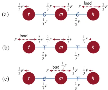
h h m t t m h m t C C T T T CFIG. 2: Force balance on the spheres and the linkers for a swimmer moving to the right, when the external loadF (act-ing to the right) is attached to the (a) head, (b) tail, or (c)
middleof the swimmer. In each case, it is identified whether each linker is undercompression(C) ortension(T), with the value of the force given (underneath).
v(t) =Aiu˙i+Biju˙iuj+Cijku˙iujuk+· · · ,where the coef-ficientsAi,Bij,Cijk,etc. are purely geometrical prefac-tors (i.e. involving only the length scalesaandℓi). After many cycles, this process gives a vanishing contribution from the linear terms ˙u1 and ˙u2and from the symmetric
combination ˙u1u2+ ˙u2u1=d(u1u2)/dt. Thus to leading
order the average swimming velocity is
V ≡ hvi= K
2hu˙1u2−u˙2u1i=K
dA
dt
, (1)
where dA is the area element in the (u1, u2) space, and
K = a
3 h 1 ℓ2 1 + 1 ℓ2 2 − 1 (ℓ1+ℓ2)2
i
[9]. In other words, to the leading order the swimming velocity is proportional to the area enclosed by the orbit of the cyclic motion in the configuration space of the deformations.
We now focus on a situation where the two arms can be in two states with deformations of either ui = 0 or
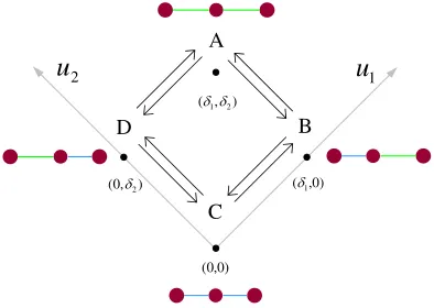
ui =δi, and transit from one to the other in an almost instantaneous fashion. This means that the configuration space of the swimmer will be made of only four distinct states as shown in Fig. 1, which correspond to different values of the pair (u1, u2), namely: state A for (δ1, δ2),
state B for (δ1,0), state C for (0,0), and state D for
(0, δ2). We then assign transition rates to the system,
corresponding to the average rate of opening and closing of the arms. For example, the transition rate from state A to state B is denoted as kBA, and similar notations are used for the 8 rates describing forward and reverse transitions along the cycle
A−−−↽k−−−BA⇀
kAB
B−−−↽k−−−CB⇀
kBC
C−−−↽k−−−DC⇀
kCD
D−−−↽k−−−AD⇀
kDA
A. (2)
For simplicity, and at the cost of motor efficiency, we as-sume that the transitions occur quite rapidly and seldom, so that they never “overlap.”
We can now calculate the swimming velocity as a func-tion the transifunc-tion rates. At steady state, the average swimming velocity of the object is given by the probabil-ity currentJ along the A→B→C→D→A cycle times the net displacement while performing the cycle. This dis-tance ∆xis simplyKδ1δ2, which yieldsV =Kδ1δ2J.The
probability currentJ is a function of the transition rates, which can be obtained from straightforward algebra:
J =P kADkDCkCBkBA−kABkBCkCDkDA
replace A by B,C,D(kADkDCkCB+kABkBCkCD+kABkADkDC+kADkABkBC)
. (3)
From the above equation it is clear that if detailed balance holds, then J is zero as the numerator van-ishes. Using the average steady state current, we can deduce the average period of one full cyclic motion along A→B→C→D→A as T = J−1. In general a 1 ←→ 2
asymmetry in the system, together with breaking the de-tailed balance at least for one of the transitions, will lead to net motion. For the particular limit where the forward rates are all much higher than the corre-sponding backward ones (kBA ≫ kAB, etc.), we find
T =k−1
AD+k−
1
DC+k−
1
CB+k−
1
BA,which simply means that the period for a full cycle is the sum of the time inter-vals needed to complete each leg of the cycle. As an-other example, we can assume that all of the equilibrium
kβα’s are equal to 1 (for the sake of illustration), and that by external action only one of them is modifiede.g.
kBA = 1 +ǫ. In this case, it is easy to show that Eq. (3) yieldsJ =ǫ/(16 + 6ǫ), which leads to a velocity pro-portional to the perturbation if the latter is small and independent of it if the perturbation is very large, as the cycling is then limited by the other three unperturbed transitions. In general, it is easy to see that the slowest leg of the reaction controls the average rate of full cyclic motion.
2 4 6 8 10 12 14 0.25
0.5 0.75 1 1.25 1.5 1.75
F δ/kBT
J(F)/J(0)
t
h m
A→Benhanced
(a)
(b)
(c)
(d)
2 4 6 8 10 12 14 0.25
0.5 0.75 1 1.25 1.5 1.75
F δ/kBT
J(F)/J(0)
m t
h
B→Cenhanced
2 4 6 8 10 12 14 0.25
0.5 0.75 1 1.25 1.5 1.75
F δ/kBT
J(F)/J(0)
t m
h
C→Denhanced
2 4 6 8 10 12 14 0.25
0.5 0.75 1 1.25 1.5 1.75
F δ/kBT
J(F)/J(0)
m
t
[image:4.612.64.558.50.173.2]h D→Aenhanced
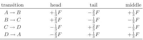
FIG. 3: Motor performance functionJ(F)/J(0) versus the external force, when only one of the rates is enhanced to 1 +ǫwhile the rest are kept fixed at 1. The plots correspond to the enhanced rate being (a) k0BA, (b) k0CB, (c) k0DC, and (d)k0AD,
and ǫ= 50. In each case, the dashed (red) line corresponds to the load being attached to thehead, the dotted (blue) line corresponds to attachment to thetail, and the solid (green) line is for themiddleattachment.
types of mechanical responses in the system. First, the external forces enter the hydrodynamic force balance on each sphere, and this will introduce a Stokes drag on the sphere as a whole, which is a linearly decaying contribu-tion to the net swimming velocity as a funccontribu-tion of force. Second, the transition rates that control the kinetics of the deformations for the two arms of the swimmer are affected by the external forces as they will have to do mechanical work against them to induce the deforma-tions. Depending on where the force is applied, different legs of the kinetic cycle could be affected, and this could lead to a complex mechanical response with the perfor-mance of the motor depending on the location of the load. The force-dependent kinetic rates will yield a net current
J(F), which combines with the Stokes response to give the swimming velocity as
V(F) =− F
18πηaR
+V0J(F)/J(0), (4)
where V0 is the swimming velocity at zero force, η is
the viscosity of the solvent, and aR is a renormalized hydrodynamic radius [10].
The transition rates are modified in the presence of ex-ternal forces, because the mechanical energy enters the balance of probability of the different states and transi-tions among them. If there is a transition from α→β
that corresponds to an extension by a factor of δ, then under a positive tension f the rate of α → β transi-tions is increased by a factor of exp(f x/kBT) while the
rate of β → α transition is decreased by a factor of exp(−f x′/kBT) where typically x = θδ is the distance
between state-αand the energy barrier andx′= (1−θ)δ
is the distance between the energy barrier and state-β
(θ between 0 and 1). Thus the ratio between the two transitions rates (i.e. the α → β rate divided by the
β → α rate) changes under a tension f by a factor of exp(f d/kBT) as required by the Boltzmann formula
(equilibrium populations between state-αand state-β un-derf).
In our system, the value of the force under which each
arm should close or open depends on where the load is applied. Figure 2 shows the break down of the mechani-cal force balance on each sphere, and the corresponding forces endured by each linker, for the three different po-sitions of the load. When the resisting force is attached to the head of the swimmer, both linkers are under com-pressional forces, and the compression force on the right arm—nearer to the load—is larger than that of the left arm by a factor of two. Attaching the load at the tail cre-ates a similar pattern of tensional forces. If the force acts on the middle sphere, the left arm is under compression and the right arm is under tension.
Using the above definition, the transition rates from a conformation stateα to another state β can be written as
kβα =k0βα exp
1 2
fβαδi
kBT
, (5)
where fβα is the force endured by the linkeri that un-dergoes a deformation during theα→β transition, and
θ = 1/2 is assumed for simplicity. The sign of fβα is determined by whether the transition (deformation) is helped (+) or opposed (−) by the force acting on the linker. The values of fβα are given in Table I for the forward reaction rates for the different locations of the load. Note that by definitionfβα=−fαβ, which can be readily used to calculate the reverse rates.
The force-dependent rates [from Eq. (5) and Table I]
TABLE I: The algebraic forcefβα which should be used in
Eq. (5) to calculate the forward rates. The values for the corresponding reverse rates can be obtained viafβα=−fαβ.
transition head tail middle
A→B +1
3F −
2
3F +
1 3F
B→C +2
3F −
1
3F −
1 3F
C→D −1
3F +
2
3F −
1 3F
D→A −2
3F +
1
3F +
[image:4.612.317.563.650.720.2]4
can be used in Eq. (3) to calculate the current J(F), which determines the swimming velocity under the effect of an external loadF. From Eq. (4), it appears that the normalized currentJ(F)/J(0) is a quantitative measure of how the ability of the motor to generate propulsion is affected by the presence of the load. In Fig. 3, this “mo-tor performance function” is plotted against the external force for the particular example discussed above (in which only one of the forward rates is enhanced to 1 +ǫ while the rest of the rates are set to unity), and δ1 =δ2 ≡δ
is assumed for simplicity. Figure 3a corresponds to when theA →B (contraction of the left arm) transition rate is enhanced, and it shows that attaching the load to the head or the middle for both of which the left arm is under a compression of 13F quickly decreases the performance of motor. On the other hand, attaching the load to the tail of the swimmer, which puts the left arm under a ten-sion of 23F, actually helps the motor initially for forces of up to 3kBT /δor so, before eventually hampering the
performance at large forces. One notes that the force across the left arm actually helps the A→B transition when the load is at the head or the middle, and opposes it when it is at the tail. It thus seems that the perfor-mance of the motor is best when the rate is enhanced for the deformation which is most hampered by the exter-nal load. In other words, the best strategy seems to be to try and make the performances of the different legs of the reaction cycle as uniform as possible, as the total velocity is controlled by the weakest performance in the cycle. The same pattern can be seen in Figs. 3b–3d. An-other interesting feature that can be seen is that when the load is at the middle and the condition is right for improved performance (see above) the system seems to endure comparatively much stronger forces: in Figs. 3b and 3c one can see that the performance is significant for loads of up to about 12kBT /δ. This is presumably
because attaching the load to the middle creates a more balanced distribution of the forces in the linkers (still of opposite nature but of equal magnitudes; see Fig. 2 and Table I).
Even when the performance of the motor is increased by the opposing force, one still has a decreasing trend for the swimming velocity because of the Stokes drag term in Eq. (4). Using a linear approximation for
J(F) ≃ J0(1 +cF δ/kBT) at small forces (where c is a
positive constant of order unity), one can write Eq. (4) as V(F) =V0
h
1− 1
18πηaRV0 −
cδ kBT
Fi, which implies that for forces much smaller than the thermal activation force kBT /δ the increased motor performance can lead
to increased swimming velocity if the viscous drag on the swimmer is larger than the thermal activation force. While this could be extremely difficult to achieve as it requires unrealistically high swimming velocities, it is an
interesting fundamental possibility that increased swim-ming velocity can be achieved upon exerting opposing forces.
In conclusion, we have proposed and studied a simple model of a low Reynolds number swimmer driven by a kinetic engine. The main result is that the ability of this swimmer to carry a load or to resist an opposing force depends on where the load or the force is applied. This is not linked to the stochastic nature of the present motor, but also holds for a motor driven by a prescribed sequence of internal stresses (to which the applied stresses add up). Altogether, this shows that the description of such machines can go beyond a simple force–velocity relation, more complex and maybe richer in functionality.
∗ Electronic address: [email protected]
[1] J. Howard, Mechanics of Motor Proteins and the Cy-toskeleton(Sinauer, New York, 2000).
[2] E.R. Kay, D.A. Leigh, and F. Zerbetto, Angew. Chem. Int. Ed.46, 72 (2007).
[3] R. Dreyfus, J. Baudry, M.L. Roper, M. Fermigier, H.A. Stone, J. Bibette, Nature437, 862 (2005).
[4] W.F. Paxton et al., J. Am. Chem. Soc. 126, 13424 (2004); S. Fournier-Bidozet al., Chem. Comm., 441-443 (2005); N. Mano and A. Heller, J. Am. Chem. Soc.127, 11574 (2005); R. Golestanian, T.B. Liverpool, and A. Aj-dari, Phys. Rev. Lett.94, 220801 (2005); New J. Phys.9, 126 (2007); G. R¨uckner and R. Kapral, Phys. Rev. Lett. 98, 150603 (2007); J.R. Howse et al., Phys. Rev. Lett. 99, 048102 (2007).
[5] G.I. Taylor, Proc. Roy. Soc. London A 209, 447-461 (1951).
[6] E.M. Purcell, American Journal of Physics 45, 3-11 (1977).
[7] A. Najafi and R. Golestanian, Phys. Rev. E 69, 062901 (2004).
[8] J.E. Avronet al., Phys. Rev. Lett.93, 186001 (2004); R. Dreyfuset al., Eur. Phys. J. B47, 161(2005); I.M. Kulic
et al.Europhys. Lett.72, 527 (2005); A. Leeet al., Phys. Rev. Lett.95, 138101 (2005); A. Najafi and R. Golesta-nian, J. Phys.: Condens. Matter17, S1203 (2005); B.U. Felderhof, Phys. Fluids18, 063101 (2006); E. Gauger and H. Stark, Phys. Rev. E74, 021907 (2006); A.M. Leshan-sky, Phys. Rev. E 74, 012901 (2006); D. Tam and A.E. Hosoi, Phys. Rev. Lett. 98 068105 (2007); D.J. Earlet al., J. Chem. Phys.126064703 (2007); C.M. Pooley and A.C. Balazs, Phys. Rev. E76, 016308 (2007); C.M. Poo-leyet al., arXiv:0705.3612; K. Kruseet al., unpublished. [9] R. Golestanian and A. Ajdari, arXiv:0711.3700.
[10] For the renormalized hydrodynamic radius in Eq. (4), we
find 1
aR = 1
a+h
1
L1i+h
1
L2i+h
1
L1+L2i − a
2h “
1
L1 −
1
L2
”2 i −
a
2h 1
(L1+L2)2i,which should be expanded in 2nd order of