Guy Vezina
December 1992
A thesis submitted for the degree of Doctor of Philosophy of
Declaration
I hereby declare that except where otherwise explicitly stated, the work presented in this thesis is my own original work.
Acknowledgments
Expressing my gratitude to everyone who contributed to my work during the last four years is almost impossible and very risky, but this is too good an opportunity.
First, thanks to my supervisor, Phil Robertson, without whom this work would not have been such an enlightening experience. His vision, inspiration and guidance have been a catalyst for my efforts, and his relentless encouragement and patience a key to my success.
My thanks also to John OCallaghan who, in conjunction with CSIRO, provided me with the support to pursue my work, and also, as members of my committee, to Robin Stan ton and Iain McLeod.
Special thanks to the people who have been a constant source of stimulation, Peter Fletcher, Don Bone and Kevin Smith. Their expertise, time and company were truly appreciated. I also thank Don Fraser and Tom Blank for many inspiring and valuable dis-cussions.
Many thanks to the members, past and present, of the visualisation group who have helped to create an exciting and challenging environment, in particular: Stephen Barrass, Jacques Blanc-Talon, Oscar Bosman, Lisa DeFerrari, Neale Fulton, Chris Gunn, Stuart Hungerford, Fei Jin, David Keightley, Simon Kravis, John Lilleyman, Chris Moran, Kevin Moore, Heinz Schmidt, Kelly Slough, Duncan Stevenson and Ken Tsui. Particular thanks to Mike Sharratt for his help and assistance in producing video clips.
Many people, perhaps unknowingly, have contributed to my work by creating a rich working environment: Dave Abel, Ross Ackland, Arch Brayshaw, Mike Clarke, Peter Fox, Paul Guignard, Mark Horn, Steve Jones, Peter Milne, Scott Milton, Pierre Nikitser, Dione Smith, John Smith and Steve Woods. Also to the administrative staff who have always given me great assistance: David Cook, Kerry Doutch, Denise Hollingsworth, Kathy Visintin and Merylin Wilmott.
To the many friends who, together with the people above, have contributed in giving me a home away from home: Jacqueline, Megan and Phil, Peter the explorer, Nikki and Chris, Ann and Chris, Bronwen and Peter, Kirsty and Steve, Judy and Adrian, Judy, and Helen. Special thanks to Mamie Merlin, who by her presence and care provided The home away from home.
Thanks to Allan Fisher from the Computer Science Department of the Carnegie-Mel-lon University for welcoming me, as a visiting student, during the beginning of my research. Thanks also to Denis Poussart and Denis Laurendeau from the Vision and Robotics Lab at Universite Laval for providing me with a great environment for pursuing my work during summer months.
Mes plus sinceres et profonds remerciements
a
mes parents, Marthe et Robert, pour leur amour et constants encouragements tout au long de ma longue carriere etudiante.Abstract
Scientific visualisation is used as an aid in data analysis, to assist in steering computations, and to facilitate the understanding of complex models and processes. Achieving interaction with visual representations is highly desired but often requires large comput-ing resources. Special-purpose architectures can provide the per-formance required but do not scale linearly with data size and
dimension. Current interactive visualisation software also lacks portability across the different high-performance platforms and re-usability towards new applications.
We base this work on image-space algorithms for the visualisation of surfaces and volumes. We address scalability and portability for interactive visualisation by exploiting a general class of
CONTENTS
1 INTRODUCTION ... 1
1.1 Scientific visualisation requirements and approaches ... 1
1.2 Visualisation framework ... 3
1.3 Organisation of this thesis ... 3
2 RELATED WORK AND BACKGROUND ... 4
2.1 Scientific visualisation ... 4
2.1.1 Image-space visualisation . . . .. . . .. . .. . . 4
2.1.2 Limitations of polygon-based algorithms ... 5
2.1.3 Specialized architectures ... 6
2.2 Data-parallel approaches ... 7
2.2.1 SIMD data-parallelism ... 7
2.2.2 A SIMD data-parallel architecture: the MasPar MP-1. ... 9
2.2.3 SIMD architecture comparisons ... 11
2.3 Multi-pass transformations ... 16
2.3.1 Decomposition techniques ... 17
2.3 .2 Scanline algorithm difficulties . . . .. . . .. . . .. . . .. .. . . 19
2.4 Resampling within spatial transformations ... 20
2.4.1 Spatial resampling requirements ... 22
2.4.2 Temporal resampling requirements ... 25
2.4.3 Reconstruction approach ... 27
2.5 Summary ... 28
3 DATA-PARALLEL FRAMEWORK ... 29
3 .1 Requirements and approaches ... 29
3.2 Multi-dimensional hierarchical design ... 29
3.3 Implementation for multi-pass scanline transformations ... 34
3.3.1 Multi-pass scanline technique ... 34
3.3.2 Algorithm mappings onto a SIMD data-parallel architecture ... 34
3.3.3 Resampling as the core component ... 36
4 SPATIAL TRANSFORMATIONS ... 41
4.1 Multi-pass resampling ... 42
4.1.1 Ideal resampling in one dimension ... 42
4.2 One-dimensional resampling implementation ... 43
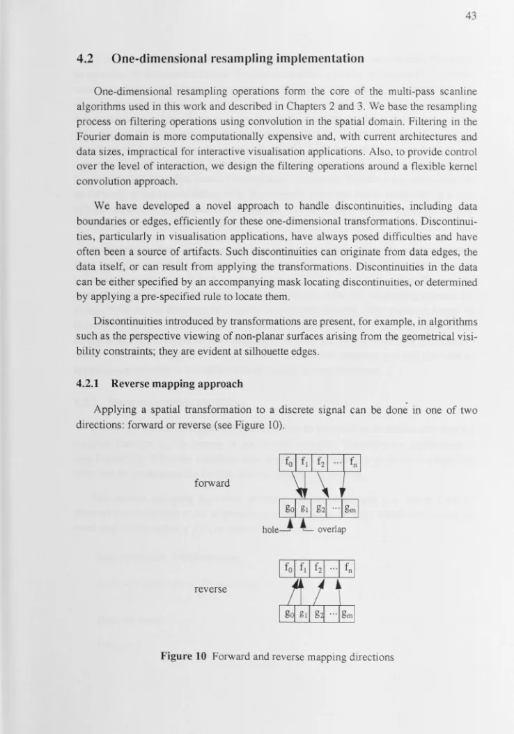
4.2.1 Reverse mapping approach ... 43
4.2.2 Reverse sampling algorithm ... 44
4.2.3 Reconstruction by convolution ... 49
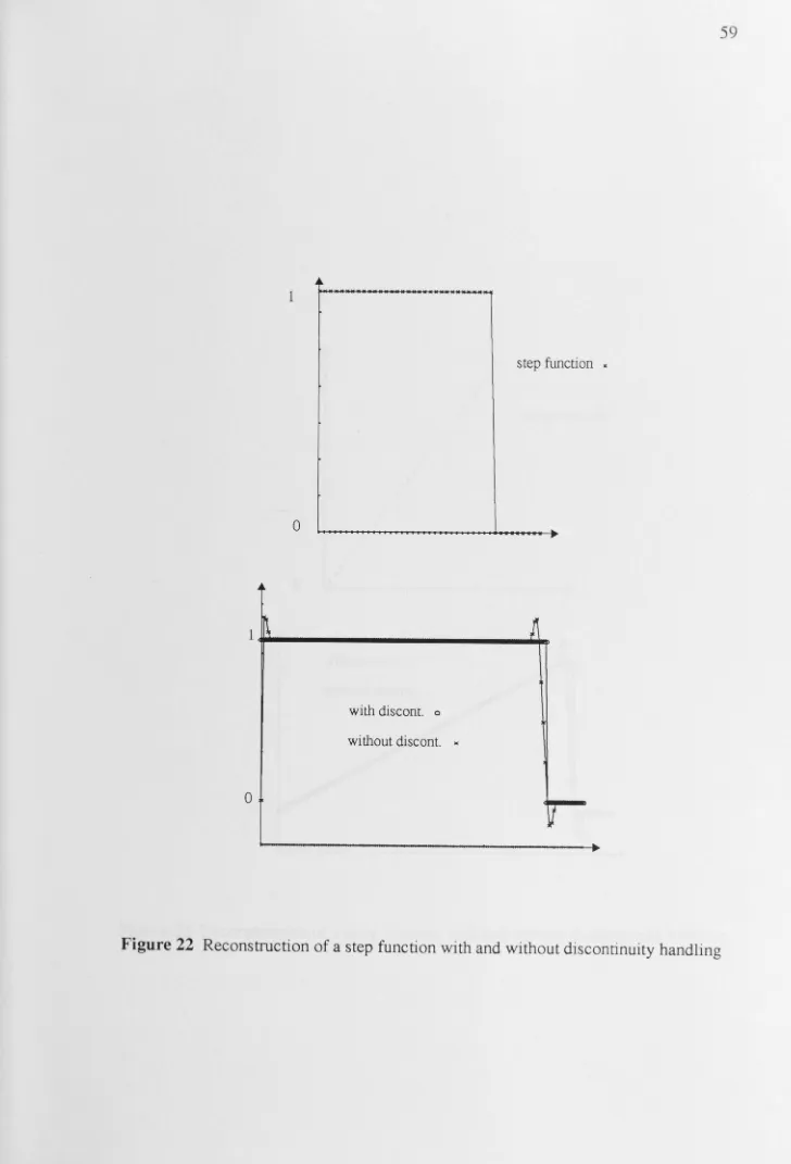
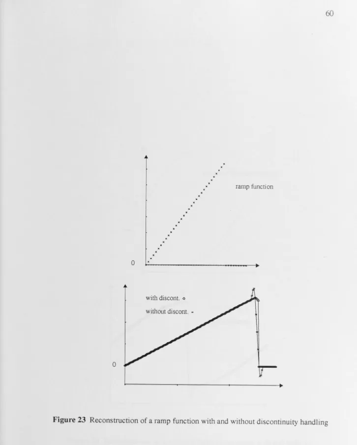
4.2.4 Edge and discontinuity handling ... 51
4.2.5 Reconstruction with embedded extrapolation ... 54
4.2.6 Test pattern reconstruction ... 56
4.3 Discussion ... 57
5 SURFACE PERSPECTIVE VIEWING ... 62
5 .1 Description of algorithms ... 62
5.1.1 Rotation ... 63
5 .1.2 Perspective projection... 65
5.2 Implementation on a SIMD data-parallel architecture ... 73
5 .3 Performance prediction and analysis ... 76
5.4 Practical results ... '. ... 79
5 .4.1 Results from the multi-pass implementation ... 79
5.4.2 Comparisons of various reconstruction filters ... 81
5 .5 Extended rendering pipeline ... 85
5 .6 Temporal resampling ... 88
5.7 Summary ... 89
6 VOLUME PERSPECTIVE VIEWING ... 90
6.1 Image-space volume visualisation ... 90
6.2 Description of algorithms ... 92
6.2.1 Rotation ... 94
6.2.2 Perspective scaling ... 96
6.3 Implementation on a SIMD data-parallel architecture ... 98
6.4 Perlormance prediction and analysis ... 101
6.5 Practical results ... 103
6.5.1 Results from the multi-pass implementation ... 103
6.5.2 Comparison with CM-2 implementation ... 106
6.6 Summary ... 107
7 CONCLUSIONS ... 108
7.1 Summary ... 108
7 .2 Achievements and limitations ... 110
7 .3 Future research ... 112
8 COLOR PLATES ... 114
List of Figures
Figure 1 Data-parallel SIMD model ... 10
Figure 2 MP-1 x-net: nearest-neighbour communication network ... 11
Figure 3 MP-1 router: global communication network ... 11
Figure 4 Two-pass scanline rotation algorithm ... 18
Figure 5 A sampling system ... 24
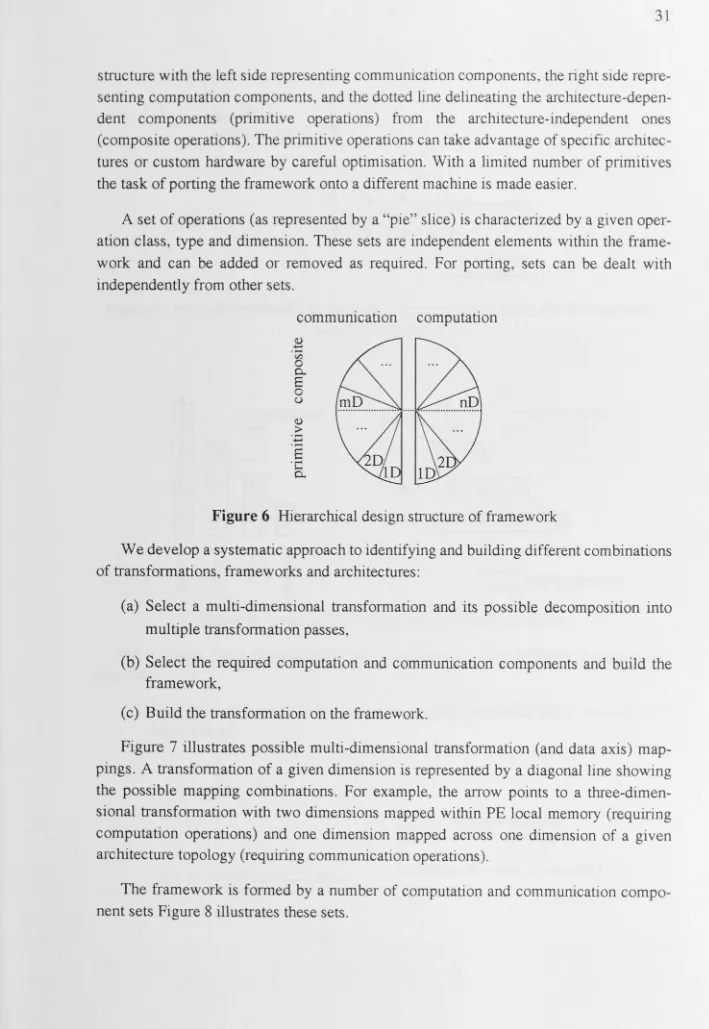
Figure 6 Hierarchical design structure of framework ... 31
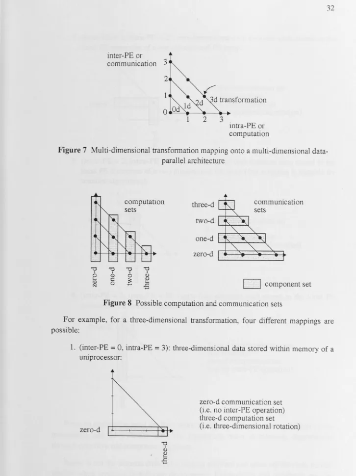
Figure 7 Multi-dimensional transformation mapping onto a multi-dimensional data-parallel architecture ... 32
Figure 8 Possible computation and communication sets ... 32
Figure 9 PE addressing autonomy ... 35
Figure 10 Forward and reverse mapping directions ... 43
Figure 11 Resampling and reverse mapping function approximation ... 45
Figure 12 Viewing geometry illustrating the projection transfo1mation ... 47
Figure 13 Profile of input data (surface heights) showing the resampled values re-quired by vertical projection with hidden-surface removal. ... 47
Figure 14 Profile of the vertical coordinates of projected data elements with hidden-surf ace rem oval ... 48
Figure 15 Profile of the output data samples following vertical projection ... 48
Figure 16 Convolution with reconstruction kernel ... 50
Figure 17 Resampling process with discontinuity handling ... 52
Figure 18 Discontinuity mask specification ... 52
Figure 19 Discontinuity mask determination ... 53
Figure 20 Linear and cubic extrapolation of missing values ... 54
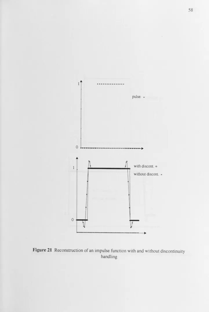
Figure 21 Reconstruction of an impulse function with and without discontinuity handling ... 58
Figure 22 Reconstruction of a step function with and without discontinuity han-dling ... 59
Figure 23 Reconstruction of a ramp function with and without discontinuity han-dling ... 60
Figure 24 Reconstruction of sinusoidal function segments with and without discon-tinuity handling ... 61
ing ... 64
Figure 27 Domain localisation for visibility determination ... 66
Figure 28 Aligned domains for projection and visibility determination ... 67
Figure 29 Vertical projection geometry ... 68
Figure 30 Derivation of the vertical projection coordinate ... 69
Figure 31 Visibility determination difficulties: folds and many-to-one mappings ... 69
Figure 32 Discontinuity introduced by folds along scanline ... 70
Figure 33 Horizontal projection geometry ... 71
Figure 34 Limitation of the viewpoint position due to the geometry ... 72
Figure 35 Discontinuities introduced by vertical projection and present before the horizontal projection pass ... 73
Figure 36 Image scanline mappings using a 4 by 4 pixel image ... 7 4 Figure 37 Partial illustration of the data movement from a single PE for transposi-tion ... 76
Figure 38 Surface rendering and viewing pipeline ... 86
Figure 39 Multiple-surf ace viewing pipeline ... 87
Figure 40 Viewing geometry of a volumetric data representation ... 92
Figure 41 Viewpoint parameters: rotation about z, y, x and distance from centre ... 92
Figure 42 Multi-pass scanline volume viewing algorithm ... 93
Figure 43 Geometry of horizontal and vertical perspective passes ... 97
Figure 44 Volume viewing pipeline including voxel shading and iso-surface classi-fication ... 98
Figure 45 Volume data scanline mapping onto a two-dimensional PE array ... 99
List of Tables
Table 1 Comparisons of arithmetic operation perlormances (peak) ... 13
Table 2 Comparisons of memory access perlormances (peak GB/s) ... 14
Table 3 Comparisons of communication perlormances (aggregate GB/s) ... 15
Table 4 Comparisons of PE to I/0 data transfer perlormances ... 16
Table 5 Kernel functions used for reconstruction ... 51
Table 6 Discontinuity handling embedded within reconstruction kernels ... 55
Table 7 Perlormance analysis for one-dimensional transformations ... 78
Table 8 Timings for one-dimensional computational components (msec) ... 80
Table 9 Timings for two-dimensional communication component (msec) ... 80
Table 10 Timings for rotation and surlace perspective viewing (msec) ... 81
Table 11 Comparative timings of filter shapes for computational components (msec) 83 Table 12 Timing for communication component: 16-bit image transposition (msec) .. 83
Table 13 Comparative timings of kernel shapes for rotation and surlace perspective viewing (msec) ... 84
Table 14 Timings of the vertical projection transformation with height fields of different frequency contents (msec) ... 84
Table 15 Timings for compositing two surlace views (msec) ... 88
Table 16 Perlormance analysis of computational components ... 102
Table 17 Perlormance analysis of transposition (with indirect addressing) ... 103
Table 18 Timings for computational components (msec) ... 104
Table 19 Timings for communication components (msec) ... 104
Table 20 Timings for three-dimensional rotation and volume perspective viewing (msec) ... 105
1
INTRODUCTION
1.1
Scientific visualisation requirements and
approaches
"The ability of scientists to visualize complex computations and simulations is absolutely essential to insure the integrity of analyses, to provoke insights and to communicate those insights with others." [McCormick et al., 1987]
Scientific visualisation is playing an important role in helping analyse, understand and explore increasing large and complex data sets and monitor complex modelling pro-cesses. It is becoming an important tool in supporting decision making in many fields.
Data sources
Increasing quantities of sensed data with advances in instrumentation and sensing devices and increasing complexity in computer modelling are creating new challenges for data collection, processing, management and understanding. Increasing levels of res-olution in spatial, spectral and temporal domains add to the quantity of data.
NASA provides a good example of the challenge ahead of us which involves the dis-ciplines of astrophysics, earth sciences, planetary sciences, space physics, life sciences and microgravity. By the turn of the century they will have to be able to handle 5000 times the annual volume of data gathered by all spacecraft only a decade ago [Green and Halem, 1990]. This is in part a result of advances in instrumentation and the larger num-ber of missions planned for the nineties. The data will amount to hundreds of terabytes in the nineties, followed with thousands of terabytes into the next century. Data rates of dif-ferent instruments used by NASA support these numbers: synthetic aperture radar (300 Mb/s), high-resolution infrared sensor (300 Mb/s), thematic mapper/multilinear array (85 Mb/s), several types of spectrometers from infrared to ultraviolet (2-30 Mb/s) and telescopes (2-10 Mb/s). NASA represents only part of the total data collection and many other organizations are involved.
Increases in data resolution and dimensionality have taken place in many fields. In remote sensing, for example, new sensing devices are capable of acquiring high
resolu-tion images in several hundred spectral bands.
Another major source of data arises from modelling physical phenomena [Patrikalakis, 1991]. In science and engineering, social science, finance and many other fields, computational modelling has become an important way of exploring and testing new ideas and theories. As supercomputer simulations become more common, not only will there be more modelling done but also greater modelling complexity will be
Common to many of these large data sets are their discrete and empirical nature, and
their multi-dimensional structure along spatial, spectral and temporal dimensions with
constantly increasing resolutions. Their high frequency contents demand that care be
taken in handling and processing them to maintain reliability in the information
process-ing. These data sets are particularly well-suited to image-space approaches [Carlbom et
al., 1991].
Interactive visualisation requirements
"Interactivity, a tool that enables scientists to steer computations. It will enrich the process of scientific discovery, lead to new algorithms, and change the way scientists do science" [McCormick et al., 1987].
Interactivity is a very powerful mechanism that allies our capacity to analyse and desire to manipulate, which in tum facilitates data exploration and understanding. The
challenge lies in our ability to handle large data sets and generate reliable visual
repre-sentations (for example as surfaces and volumes).
Interactivity relies on high capacity storage, powerful processing and high bandwidth display components. Interactive visualisation frameworks should perform efficiently and
be portable across various architectures. If interactivity is to be maintained on progres-sively larger data sizes or complex models, an approach that allows us to take advantage of the highest performance computers, and scales with increased computer resource, is
required. Massively data-parallel computing offers performance scalable with data size if
scalable data-parallel algorithms are used.
Image-space approaches
"The increase in model complexity will influence a radical change in the design of graphics hardware and the graphics pipeline ... the logical conclusion is that hardware must migrate from polygon algorithms to pixel algorithms based on true geometries." [Greenberg, 1991]
Visualisation algorithms are often characterized as working either in object-space or
image-space. With large increases in the amount of data to be handled, both from
model-ling and sensing sources, object-space visualisation systems face limitations associated with performance scaling, particularly when rasterization is involved. Image-space
approaches need not suffer these constraints. This is particularly true when dealing with
1.2
Visualisation framework
We focus on addressing the scalability and portability issues of interactive visualisa-tion by exploiting a general class of emerging data-parallel high-performance architec-tures. We concentrate on the spatial transformation requirements found in several visualisation algorithms. Using the image-space approach, we follow the principles of decomposing spatial multi-dimensional transformations into one-dimensional core resa-mpling components and reducing the transformation fidelity problems to generic well-posed resampling problems. This technique is particularly well-suited to massively data-parallel processing given its scope for regularizing processing and localizing data access. Using a data-parallel SIMD model, we integrate these components within a general framework which offers flexibility, portability and extensibility while maintaining per-formance. The framework is demonstrated on widely used visualisation algorithms for surface and volume viewing.
1.3
Organisation of this thesis
Chapter 1 has introduced the major requirements underlying this work, and outlined the approach taken to meeting these requirements.
Chapter 2 summarizes more fully the limitations of cun·ent visualisation algorithms in achieving scalable performances, data-parallel approaches, and key features of data-parallel algorithms and architectures that determines their suitability for interactive visu-alisation using image-space algorithms. The key aspects of these algorithms, their offer of a regularized domain for resampling, is then described together with relevant resam-pling issues and the importance of flexible filtering techniques. Multi-pass algorithms, and their decomposition into core components, are described with their uses and out-standing problems.
Chapter 3 presents a framework for portable data-parallel visualisation algorithms designed to meet the shortcomings of existing approaches and allow flexibility in appli-cation and implementation on different data-parallel architectures.
Chapter 4 describes in detail the approach taken to providing flexibility in resam-pling in the multi-pass algorithms, as well as the overall framework, describing theoreti-cal and practitheoreti-cal requirements and the compromises adopted.
Chapter 5 provides an example of the developed approach for a set of surface view-ing algorithms, with implementation on a massively data-parallel SIMD machine, and perlormance analysis.
2
RELATED WORK AND BACKGROUND
2.1
Scientific visualisation
Interactive visualisation of all but the simplest of data requires supercomputing lev-els of performance and high data bandwidths. Performance and scalability requirements suggest the use of parallel architectures and image-space algorithms. Image-space algo-rithms can also regularise the problem of fidelity associated with data transformations, allowing a consistent approach to minimising artifacts that arise from the visualisation process.
This chapter expands on the reasons for choosing image-space algorithms and briefly considers specialised architectures that have been developed to provide high pe1for-mance for visualisation applications. General data-parallel architectures and algorithms are also described, and general purpose SIMD massively data-parallel computers are compared with key features on which we build our framework. Particular features of the MasPar MP-1 that help to regularise the use of data-parallel computers are explored.
We then treat the background to the transformation fidelity problem in more detail, addressing resampling in image transformations and requirements for avoiding visual artifacts, and describing work relevant to resampling within a data-parallel image-space visualisation framework. We then describe a class of image-space algorithms, multi-pass scanline algorithms, within which regularised data-parallel resampling can be incorpo-rated. These algorithms have a natural mapping to massively data-parallel architectures and cover many image processing and visualisation operations. We use multi-pass algo-rithms as the link between requirement for interactive visualisation, the performance
offered by massively data-parallel architectures, and the need for a consistent framework for resampling. Previous work with these algorithms is summarised in this chapter.
2.1.1 Image-space visualisation
Visualisation and computer graphics algorithms are characterized as working either in object-space or image-space [Sutherland and Hodgman, 1974]. Object-space algo-rithms (also referred to as polygon-based algoalgo-rithms) manipulate geometrical objects or
sub-objects defined within an object modelling framework. Image-space algorithms manipulate ( object) data samples at a picture element (pixel) or volume element (voxel) level and can be applied to work at the maximum available data resolution.
object-space approaches is often algorithm-dependent while in an image-based approach opera-tion complexity can be data-dependent. This affects perlormance scalability of algo-rithms when large data sets are to be used.
2.1.2 Limitations of polygon-based algorithms
Polygon-based algorithms in general seldom scale gracefully with data size [Green-berg, 1991], can provide difficult resampling problems, and seldom parallelise well on massively data-parallel SIMD architectures.
Object-space approaches to visualising empirical image data require modelling of the data using a polygonisation or tessellation approach. This can be expensive, particularly with large data sets. In surlace representation algorithms, object-space approaches approximate empirical image data as polygon mesh surlaces, as parametric surlaces, or as quadric surlaces. Modelling surlaces or computing connecting surlace patches is expensive, and manipulating them for operations such as visible-surlace determination can become prohibitively expensive as data size increases. Many algorithms for visible-surlace determination do operate in object-space and require significant processing capa-bilities resulting in the design of special-purpose architectures.
Following the determination of visibility, shading and rasterising (or scan-convert-ing) the patches for display is required. Rasterising transforms the geometric description of an image into pixels for raster-scan displays. Rasterisation includes the conversion of two-dimensional vectors and three-dimensional polygons (often triangles). The tech-niques involved influence the interactivity (or update rate) and depend on image com-plexity and display resolution. These techniques involve many difficulties particularly across an edge between adjacent patches or polygons or when an edge corresponds to a ridge in the scene (e.g. top of a hill) such that one side faces towards the light source and the other one away from it [Coquillart and Gangnet, 1981; Max, 1989]. The discontinui-ties found in the shading function, or its derivatives, reveal the problems involved with surlace approximation and modelling. To alleviate these, higher degree interpolation is often required and smoothing of boundaries often done which may affect representation fidelity. The conversion is subject to errors which are difficult to predict since they depend on the image complexity [Bregt et al., 1991]. This is another reason why object-space approaches on empirical data do not always provide a desirable solution.
Greenberg [1991] raised another argument in support of image-space approaches. Size increases of complex models and sensed data are greater than the increase in display resolution. In an object-space approach the average number of pixels covered per
poly-gon reduces to only a few. Scan-converting such polypoly-gons requires major computations since most pixels cover edges. In such a situation it is preferable to work in image-space
at maximum resolution.
The cumulative effect of these constraints makes interactive manipulation of large data sets with object-space algorithms difficult, and perlormance scalability unachiev-able. To address these limitations we adopt an image-space approach.
2.1.3 Specialized architectures
The traditional approach to high performance graphics has been to use a pipelined "geometry engine", comprising one or more pipes of fast transformation hardware to perform high speed polygon/point affine transformations and scan-conversion, including region fill and various other options. This follows a typical graphics object modelling pipeline incorporating sets of viewing and other transformations.
This kind of architecture has been widely used for problems up to tens or hundreds of thousands of polygons, and enormous effort has gone into finding efficient intersection and visibility algorithms, efficient antialiasing, and other techniques. As described ear-lier, because in general these algorithms do not scale gracefully, it becomes increasingly difficult to achieve interactive perlormance as data size or complexity increase [Green-berg, 1991].
Several special-purpose architectures have been designed for more generalised com-puter graphics and image processing. Visualising volumetric images (of the order of gigabits for moderate spatial resolution) has been the focus of several of these architec-tures.
Published architectures include [Kaufman, 1990] the Voxel processor which is a pipeline of parallel rendering processors [Goldwasser and Reynolds, 1987], the 3DP which is a hierarchical pipeline of processors [Ohashi et al., 1985], the Cube architecture which has a skewed memory feature and three dedicated processors [Kaufman and Bakalash, 1988], the Insight which has an octree-based solid engine [Meagher, 1985], the AT&T Pixel machine which has both linear pipes and a two-dimensional array of digital signal processors with interlaced frame buffer [Potmesil and Hoffert, 1989], the Pixar machine which is composed of four specialized processors operating in parallel in a SIMD fashion [Levinthal and Porter, 1984], the Pixel-planes 5 which is a raster graph-ics engine incorporating custom logic-enhanced memory chips [Fuchs et al., 1989], the Silicon Graphics 4D which has a higher level geometry architecture and a lower level pixel-parallel architecture [Akeley, 1989], and the T AAC-1 accelerator [McMillan,
1989].
2.2
Data-parallel approaches
Data-parallel architectures are becoming a major focus in supercomputing because
they can potentially overcome the limitations that have been reached with scalar and
vec-tor processors. Advances in architectures and computing paradigms are complicated by
technological and engineering constraints such as propagation delays, power dissipation and logic gate area [Hockney and Jesshope, 1988]. Pipelined vector computers have long
held the supercomputer market because fast logic was more affordable than large
memo-ries and communication requirements of parallel architectures. But in the 1980's this has
changed. The physical limits of high performance single components, such as CPUs, are
approaching; performance improvements depend more and more on parallelism.
Tech-nology now allows easy VLSI integration of logic and memory, raising new issues about processor/ memory balance and communications. Overall the numbers of researchers,
publications, and conferences are increasing while commercial systems are becoming mature. It is well accepted that parallelism holds the key to the future of high perfor-mance computing. Effective exploitation of parallelism relies on developing parallel approaches and algorithms to problem solving.
The hardware technology is thus maturing while the software environment still requires much attention. Realising that our software investment is often more significant that the hardware, we focus on designing and developing a software framework that can
exploit a class of parallel architectures.
Many visualisation algorithms can be performed using parallel processing approaches. In object-space, objects can form the basis for parallelisation. Parallelisation of object-space algorithms is dependent on the application and does not lend itself easily
to generic approaches. Many image-space algorithms offer better parallelisation
ave-nues. In our work, we have found that data-parallel domains extracted along orthogonal data dimensions offer efficient parallelisation schemes; particularly with data-parallel architectures [Vezina and Robertson, 1991; Vezina et al., 1992c].
2.2.1 SIMD data-parallelism
We focus on the SIMD (single instruction multiple data) model of data-parallelism. It consists of distributing the data across many processing elements. Its regular and simple
structure provides a basis for well engineered software as we address scalability with
respect to the data, the algorithms and the architectures.
Several attempts have been made at classifying parallel architectures [Hockney and J esshope, 1981]. The Flynn nomenclature is possibly the most used [Flynn, 1972].
Rather than surveying the field in general, we consider system capabilities and their
suit-ability to image-space visualisation algorithms with particular emphasis on their extent,
We address key aspects of data-parallel architectures that make the machines suitable platforms for image-space visualisation. The desired level of parallelism, or granularity,
is first considered. It applies to both processors and problems. Processor granularity refers to the relative "size" and number of the processing elements (PEs), and problem granularity refers to the amount of work done in parallel by each PE. Problem granularity is determined by considering the problem breakdown into parallel domains with respect to the costs involved in balancing parallelism against communication time requirements.
Virtualisation of the number of PEs, the process of mapping more than one logical PE to /
each physical PE, involves fragmenting local memory and complicates the usefulness of such measures. Efficient problem mappings onto machines depend not only on the gran-ularity but also on the size of the memory and the power of each PE.
To determine the desired processor granularity we estimate the problem granularity for image-space visualisation applications. Typical data sets range from a single image of between 1002 and 10K2 picture elements (pixels) to multiple images. In
three-dimen-sional data sets, volumes can range from 1()3 to 10003 volume elements (voxels). These large numbers, combined with the processing involved, lead us to massively data-paral-lel architectures, i.e. fine-grained machines. Granularity and scalability issues are further discussed when mapping our algorithms onto a data-parallel architecture, and an analysis of problem-size/ machine-size combinations is also presented.
Having focussed on massive parallelism we look at the mode of parallelism. Since the transformations we consider exhibit a high level of regularity on well-structured par-allel domains, a single-instruction-multiple-data (SIMD) model is chosen. SIMD archi-tectures can be considered, for programming, in the same way as a sequential computer since only one instruction is executed at any time; this eases software portability. This is in contrast to multiple-instruction-multiple-data (MIMD) computers in which program-ming is often a more difficult task because communication must be handled explicitly and often asynchronously with any one processor instruction sequence.
Amongst SIMD architectures, several processor array topologies exist. Many topolo-gies allows us to exploit the regular structure of image data. These topolotopolo-gies consist of orthogonal arrays such as one-dimensional arrays (CLIP7 A [Fountain et al., 1988],
SLAP [Fisher and Highnam, 1985]), two-dimensional arrays (ILLIACIV [Slotnick,
1971], DAP [Reddaway, 1973], MPP [Batcher, 1980; 1985], CM-2 [Hillis, 1985], MasPar MP-1 [Blank, 1990]) and three-dimensional arrays ([Wavetracer, 1991]). Such a diversity of topologies makes generic communication approaches difficult.
smallest communication complexity - this is mainly due to the inherent topological matching between a mesh network and the required two-dimensional search area of many algorithms [Fang et al., 1989].
Also, these architectures can be characterised in terms of PE autonomy in:
addressability,
controllability,
connectivity.
Autonomy in addressing allows each PE to access different locations in their local memory. Autonomy in control allows each PE to execute different instructions. Auton-omy in connections allows each PE to communicate with different PEs. The first mas-sively parallel architectures to embody some level of PE autonomy were the CLIP and MPP [Batcher, 1980] with the CLIP7 A architecture allowing complete addressing auton-omy of data sources and some flexibility in selecting the function to be executed at each PE.
While much emphasis has been put on hardware development, software development environments are less well developed and are recognized as the key to wide acceptability of parallel machines [Siegel, 1990]. We do not discuss the relative merits of the different systems. We do, however, present a software framework that takes into account the need for better programming support embedded with current massively parallel operating environments.
2.2.2 A SIMD data-parallel architecture: the MasPar MP-1
A series of designs and machines have been realised in the past, all with their own features and peculiarities. SIMD data-parallel architectures, such as the massively paral-lel MasPar MP-1, have shown better performances than conventional vector computers such as the Cray on well-structured problems such as signal processing algorithms [Rover et al.].
The SIMD model, a distributed memory machine, typically consists of a set of PEs,
each with its own local memory, an inter-PE communication scheme and a control unit. The control unit broadcasts instructions to all PEs, and each active PE executes these instructions on its local memory. Instructions are executed simultaneously. The commu-nication scheme allows PEs to exchange data and can include an interconnection net-work and/or shared memory.
The MP-1 computer [Blank, 1990] contains a sequential controller machine (ACU)
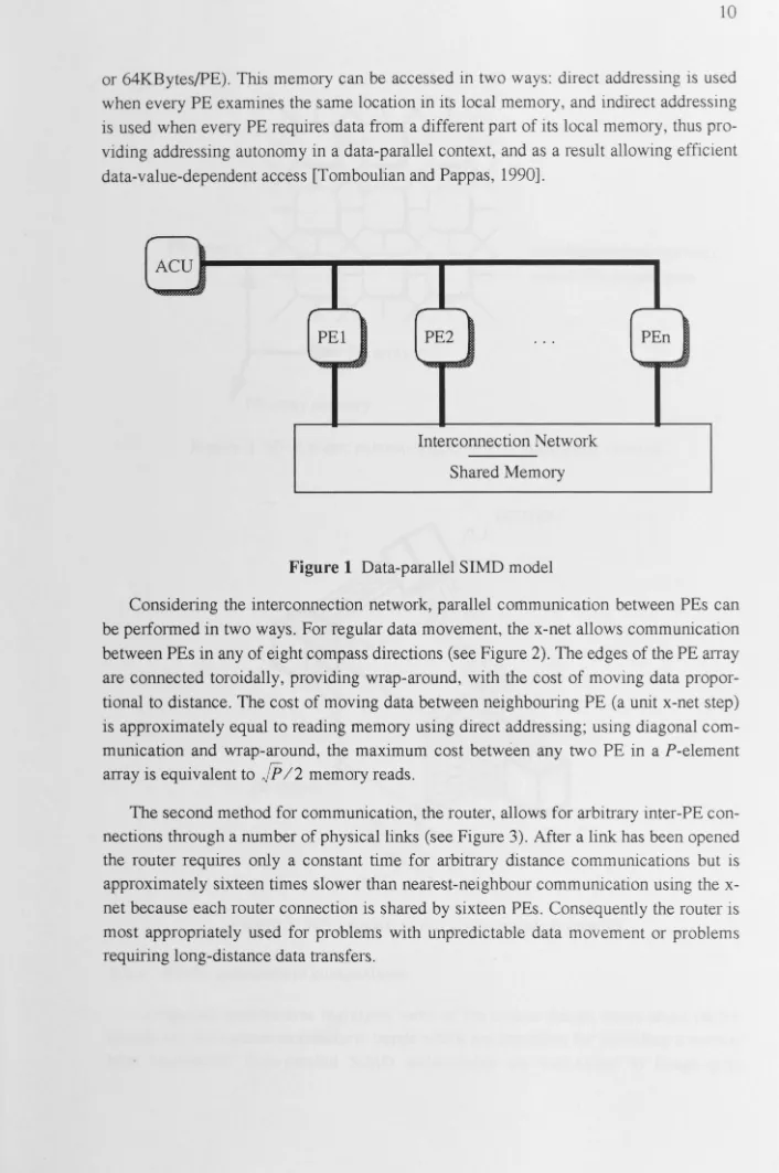
or 64KBytes/PE). This memory can be accessed in two ways: direct addressing is used when every PE examines the same location in its local memory, and indirect addressing is used when every PE requires data from a different part of its local memory, thus pro-viding addressing autonomy in a data-parallel context, and as a result allowing efficient data-value-dependent access [Tomboulian and Pappas, 1990] .
r ...,
ACU \..
r ..., r .,
PEI PE2 ... PEn
"- \..
..
\.Interconnection Network Shared Memory
Figure 1 Data-parallel SIMD model
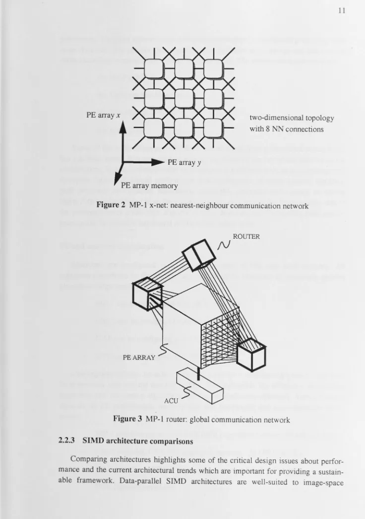
Considering the interconnection network, parallel communication between PEs can be performed in two ways. For regular data movement, the x-net allows communication between PEs in any of eight compass directions (see Figure 2). The edges of the PE array are connected toroidally, providing wrap-around, with the cost of moving data propor-tional to distance. The cost of moving data between neighbouring PE (a unit x-net step) is approximately equal to reading memory using direct addressing; using diagonal com-munication and wrap-around, the maximum cost between any two PE in a P-element array is equivalent to
jp
/2 memory reads. [image:20.761.30.736.31.1094.2]PE array x
1---~
PE array yPE array memory
[image:21.759.8.744.22.1068.2]two-dimensional topology with 8 NN connections
Figure 2 MP-1 x-net: nearest-neighbour communication network
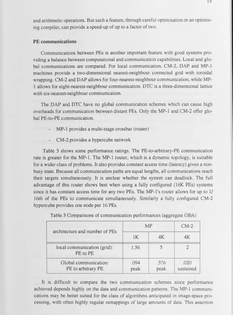
ROUTER
j\)
PE ARRAY
Figure 3 MP-1 router: global communication network
2.2.3 SIMD architecture comparisons
processing. They can achieve peak performances on highly regularized processing over large data sets. We present four commercially available architectures and characterize them according to some of the criteria exposed above. The architectures discussed are
the MasPar MP-1,
the Thinking Machine CM-2,
the WaveTracer DTC,
theAMTDAP.
Some of the information provided here was obtained from promotional material and has not been tested. It is provided to give an overview of the key characteristics of the architectures. Benchmarking parallel architectures is a difficult task, as is comparing per-formance figures. Achieved perper-formance is a combination of many aspects, including peak processor performance, realistically achievable processor perlormance on typical tasks, data bandwidth to/ from the processor array, data bandwidth between elements of the processor array under high and low volume demands, etc. Comparing peak perlor-mances can be valuable but should not be solely relied upon.
PE and memory configuration
Machines are configured with varying numbers of PEs and local memory. All machines considered in this comparison can safely be classified as massively parallel given their large number of PEs.
MP-1 can be configured with lK to 16K PEs,
CM-2 can be configured with 4K to 64K PEs,
DAP can be configured with lK to 4K PEs, ·
DTC can be configured with 4K to 16K PEs.
One important design issue in configuring a system is maintaining a balance between local memory size and the number of PEs. This influences the efficiency of handling large data sets for certain algorithms and the parallelisation approach. Such a balance depends on PE performance, memory size and bandwidth, and communication band-widths.
MP-1 provides either 16 or 64 KB/PE (aggregate memory 16 MB to 1 GB),
CM-2 provides 32KB/PE (aggregate memory 128 MB to 2 GB),
DAP provides 16KB/PE (aggregate memory 64 MB to 256 MB),
If more memory is required for a problem it can be achieved by adding more
proces-sors or increasing the size of local memory. Relative benefits are influenced by having
more processing power and the costs of added communication.
PE performance characteristics
The width in bits of the serial processors making up the PE is not directly relevant to
the design of algorithms except when considering extensive optimisation schemes such
as taking advantage of bit packing. These features are most relevant when contemplating the performance scalability of architectures (increase in data path widths offers scope for
increased performance).
MP-1 PE has a 4-bit serial processor,
CM-2 PE has a 1-bit serial processor (also one floating-point processor for
every 32 PEs),
DAP PE has a 1-bit serial processor (also now 8-bit PE with its CP8 option),
DTC has a 1-bit serial processor.
The four systems are thus not necessarily directly comparable on a number-of-PE basis, nor is it fully appropriate to compare lK MP-1 systems to 4K DAP and CM-2
sys-tems. These differences are not critical in our design since we use languages that abstract such features. What is important is the functionality and performance that such proces-sors offer. Relevant comparisons depend on whether, for a particular algorithm, the per-PE performance is adequate in data access bandwidth, fixed-point and floating-point per-formances.
PE perfo1mance can be measured by its ability to compute 32-bit integer addition
(MIPS) and its 32-bit floating-point addition/multiplication average performance (MFLOPS) (see Table 1, note that performance ratings were not available for DTC).
Table 1 Comparisons of arithmetic operation performances (peak)
MP-1 CM-2 DAP
architecture and number of PEs
lK 4K 4K lK
32-bit integer add (MIPS) 1875 7500 150 105
32-bit floating-point add/mult. avg.
94
375 357 121(MFLOPS)
The MP-1 shows an advantage on integer additions (50 times faster) over the CM-2
(DAP timing with the CP8 8-bit co-processor). All ratings are reported as scalable with
the number of PEs. It should be noted that the MP-1 floating-point rating may be more realisable than that of the CM-2 because the CM-2 is configured with one floating-point
processor per 32 PEs. For computation with regular floating-point load per PE (as is
typ-ical in image processing) a bottleneck in getting data to/ from the floating-point
proces-sor may result, with subsequent performance drop, particularly when data movement
operations are high.
An important comparison, for the design of algorithms, is the relative performance of
fixed-point versus floating-point arithmetic. MP-1 PE fixed-point precision calculations are 20 times faster than their floating-point counterparts. For the CM-2 floating-point operations can be performed twice as fast as fixed-point operations. The DAP provides comparable performance on fixed-point and floating-point operations. These perfor-mances should influence the design of our algorithms; e.g. on the MP-1 we may want
computations to be performed on a fixed-point basis, while on the CM-2, floating-point
based computations may be more desirable. In order to design efficient and portable applications we need to reduce the dependencies on architecture characteristics to a
min-imum.
A critical issue affecting the design and implementation of spatial transformation algorithms, described later in this work, is the PE-to-memory access performance. Table
2 shows that using direct memory addressing, the DAP provides the best performance per PE. The MP-1, however, provides the capability of indirect addressing (addressing
autonomy) which can be of significant value because it allows data-dependent memory addressing. This feature not only provides efficient algorithm implementations but also eases the programming task. The CM-2 does also allow the indirect addressing of arrays
through its programming language based on C (C*) but provides poor performances (even through the use of CM-2 specialised libraries). Indirect addressing turns out to be a
highly desirable feature since it can offset the stringent re_quirements for communication.
Table 2 Comparisons of memory access performances (peak GB/s)
MP CM2 DAP DTC
architecture and number of PEs
lK
4K
4K
lK
4K
aggregate PE-memory:
direct addressing 0.75 3 2.3 1.28
4
indirect addressing 0.25 1 n/a n/a n/a
aggregate PE-register 7.3 29.25 n/a n/a n/a
The MP-1 also allows memory load / store operations to overlap with PE
and arithmetic operations. But such a feature, through careful optimisation or an optimis-ing compiler, can provide a speed-up of up to a factor of two.
PE communications
Communications between PEs is another important feature with good systems pro-viding a balance between computational and communication capabilities. Local and glo-bal communications are compared. For local communication, CM-2, DAP and MP-1 machines provide a two-dimensional nearest-neighbour connected grid with toroidal wrapping. CM-2 and DAP allows for four-nearest-neighbour communication, while MP-1 allows for eight-nearest-neighbour communication. DTC is a three-dimensional lattice with six-nearest-neighbour communication.
The DAP and DTC have no global communication schemes which can cause high overheads for communication between distant PEs. Only the MP-1 and CM-2 offer glo-bal PE-to-PE communication.
MP-1 provides a multi-stage crossbar (router)
CM-2 provides a hypercube network
Table 3 shows some performance ratings. The PE-to-arbitrary-PE communication rate is greater for the MP-1. The MP-1 router, which is a dynamic topology, is suitable for a wider class of problems. It also provides constant access time (latency) given a non-busy state. Because all communication paths are equal lengths, all communications reach their targets simultaneously. It is unclear whether the system can deadlock. The full advantage of this router shows best when using a fully configured (16K PEs) systems since it has constant access time for any two PEs. The MP-1 's router allows for up to 1/
16th of the PEs to communicate simultaneously. Similarly a fully configured CM-2 hypercube provides one node per 16 PEs.
Table 3 Comparisons of communication performances (aggregate GB/s)
MP CM-2
architecture and number of PEs
lK 4K 4K
local communication (grid): 1.56 5 2
PE to PE
Global communication: .094 .376 .020
PE to arbitrary PE peak peak sustained
[image:25.777.12.763.36.1050.2]
'-would require substantial testing to be considered conclusive. We also would expect the hypercube performance to be in general more data-dependent.
PE array control mode
All systems are SIMD synchronous architectures. The MP-1 and DAP use a control-ler to decode and send instructions to their PE arrays. The CM-2 and DTC systems rely on the host computer for instruction fetching, decoding and broadcasting to the PE array. These differences do not affect the design of our applications but in a real visualisation application environment they should be taken into account (e.g., it may be desirable to have the host computer working asynchronously from the PE array since it may allow the host to handle the user interlace). Also important in a visualisation environment is the machine user-sharing capability. While some of these architectures are becoming more affordable, they remain too costly for personal use. The CM-2 allows a multi-user mode by assigning different PEs to different users, and allows up to four connected hosts. The DAP allows memory to be partitioned amongst several users, as does the MP-1. These considerations affect usability of our visualisation applications.
1/0 performance
We compare the suggested I/0 performances of the different data-parallel architec-tures. PE to I/0 communications on the MP-1 use the global router. The DAP uses a spe-cial data plane through which entire data planes can be transferred to I/0. Aggregate rates are provided in Table 4. For interactive display or animation with refresh rates of 30 frames/sec, a 10242 24-bit pixel colour image requires a data transfer rate of 90MB/sec.
Table 4 Compa:iisons of PE to I/0 data transfer perlormances
MP1 architecture and number
of PEs
lK 4K
PE to I/0 (MB/sec) 94 peak 360 peak
1 predicted performance only
2.3
Multi-pass transformations
CM-2
4K
50 peak
DAP
lK
38 sust.
transfer-mati.ons are at the basis of several geometrically-based applications such as scaling,
rota-tion and projecrota-tion. A spatial transformarota-tion defines a spatial mapping from coordinates
in input space to coordinates in output space.
Before addressing resampling techniques which form the basis of spatial
transforma-tions, we now present the basis onto which our framework is designed. Multi-pass
trans-formations provide the means to implement efficiently the spatial transformations
required in many visualisation algorithms. They also lend themselves to efficient
data-parallel mappings.
Separable multi-dimensional transformations can be decomposed into a sequence of
lower-dimensional transformations; such a sequence is called a multi-pass transforma-tion. Scanline algorithms implement multi-pass transformations with a sequence of
one-dimensional (scanline) transformations operating along orthogonal data axes. Such an
approach provides regular and predictable data accessing and localized data processing. Using this approach, multi-dimensional transformations have been implemented
effi-ciently on machines with limited capabilities on memory and communication bandwidth (particularly with respect to I/0 bandwidth).
Multi-pass transformations can be implemented exactly if they are separable; allow-ing each data dimension to be sampled independently. For scanline transformations this reduces the resampling requirements to one-dimensional resampling operations. Scan-line algorithms include separable transformations such as two-dimensional rotations,
texture mapping transformations, and image warping [Fraser and O'Brien, 1979;
Cat-mull and Smith, 1980; Weiman, 1980; Friedmann, 1981; Paeth, 1986; Tanaka et al., 1986; Hanrahan, 1990]. Other transformations such as Hough transforms [Fisher and Highnam, 1987] and two-dimensional FFT [Gonzalez and Wintz, 1977] have been implemented in a scanline manner successfully. Approximate decompositions have also
been implemented for the perspective projection of surfaces with hidden-surface
removal [Robertson, 1987; 1989].
2.3.1 Decomposition techniques
A generalized decomposition technique was presented by Catmull and Smith [1980]. The technique can be briefly outlined as follows using a notation similar to Smith
[1987].
Given the input data coordinates:
with x and y as the mapping functions. We want as a first pass the mapping x' such that we obtain the intermediate coordinates:
and, as a second pass, the mapping y' such that:
Thus we get a horizontal transformation/ such that:
and a vertical transformation g by solving
Note that decomposition of a two-dimensional transformation is not limited to a sequence of two passes. An example where a two-dimensional transformation (rotation) is decomposed advantageously into three passes (shears) can be found in [Paeth, 1986; Tanaka et al., 1986].
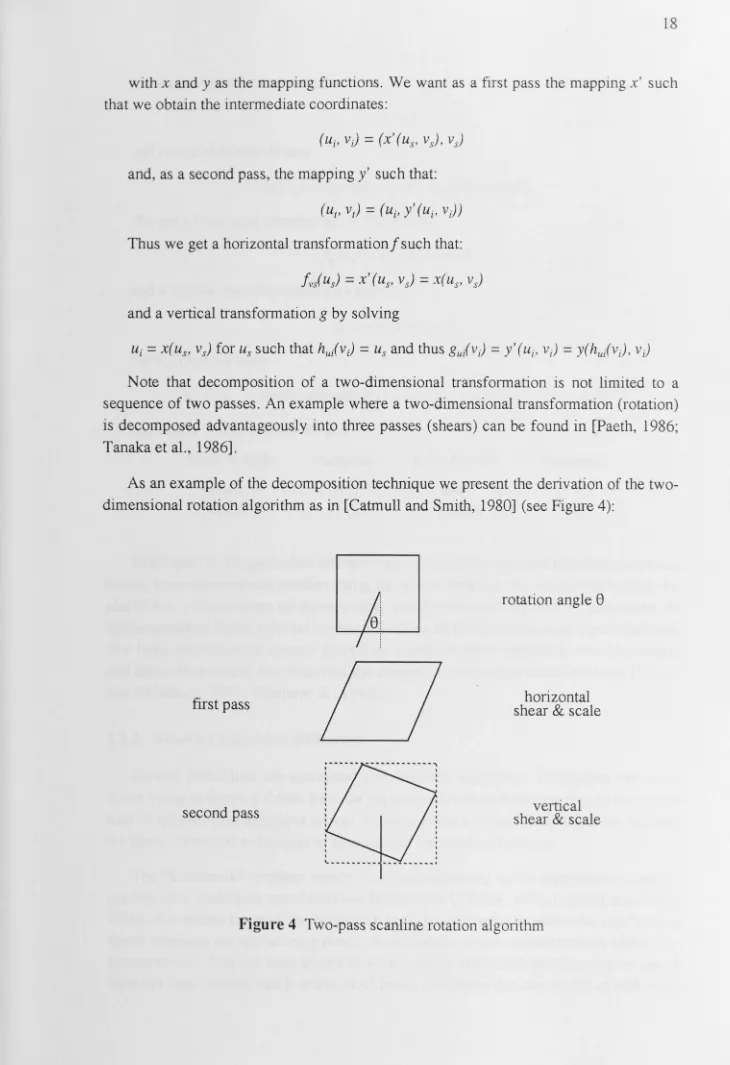
As an example of the decomposition technique we present the derivation of the two-dimensional rotation algorithm as in [Catmull and Smith, 1980] (see Figure 4):
first pass
second pass
' ' '
' ' '
~---
---·rotation angle
e
horizontal shear & scale
[image:28.755.14.744.18.1083.2]vertical shear & scale
Given the input data coordinates:
and output data coordinates:
We get a horizontal transformation/ such that:
and a vertical transformation g by solving:
for us. Thus we have:
us= (ui - vs sin8)/cos8 and gulv) = -((ui - vs sin8)/cos8)
+
y cos8Expressed in matrix form we get: shear & scale
I
cos8~
L-sin8Ij
transpose shear & scale
I
tan8~
L1 I ( cos8)I
j
transpose
In Chapter 6, we generalise this technique to three-dimensional transformations and
derive three-dimensional rotation using the above notation. As mentioned before, our
aim is not to concentrate on decomposing transformations but rather on addressing the
implementation issues relevant to the resampling of these decomposed transformations. We have implemented several multi-pass transformations including two-dimensional
and three-dimensional data rotations and perspective projection transformations [Vezina
and Robertson, 1991; Vezina et al., 1992c].
2.3.2 Scanline algorithm difficulties
Several difficulties are associated with scanline algorithms. Difficulties can occur
when trying to derive a closed form for the required inverse functions (e.g. in the second
pass of the two-pass technique above). In cases where a closed-form cannot be obtained, we chose numerical techniques to approximate the required function.
The "bottleneck" problem results from undersampling in the intermediate transfor
-mations of a multi-pass transformation [Fraser and O'Brien, 1979; Catmull and Smith,
1980]. For severe cases of the bottleneck problem, the order in which the intermediate transformations are applied may require modification, or pre-transf01mations added (e.g. transposition). This has been shown to work in many bottleneck problems but no proofs
rotation algorithms provide a good theoretical basis for understanding this problem
[Thong, 1985; Fraser, 1987; 1989; Fraser and Schowengerdt, 1992]. Studies for more
complex transformations, such as non-planar transf01mations, are desirable but pose
sev-eral difficulties due to possible discontinuities involved.
The "foldover problem" affects the mathematical derivation techniques used for
decomposition and is due to many-to-one transformation mappings. These mappings
make the inverse functions, required in certain multi-pass algorithms, multi-valued. Let
us consider the perspective projection of surlaces from three dimensions to two dimen-sions. If the surface is planar then no foldover problem occurs, but if the surlace is
non-planar, then foldovers ( or self-occlusion) can occur. This problem arises in the
hidden-surlace problem found in several viewing transformations [Sutherland and Hodgeman,
1974; Robertson, 1987]. We solve this by providing a many-to-one mapping resolution
method with each mapping.
Added to problems associated with non-separable transformations there is also a
problem associated with the separability of resampling filters. Filters are often non-separable (e.g. circularly symmetric ones) thus a multi-pass technique will only approxi
-mate the single-pass filter. This is one of the many trade-offs that must be considered.
Finally, extra aliasing problems can be introduced as a result of reducing the multi-dimensional resampling process to one-multi-dimensional processes. This happens
irrespec-tively of whether the transformation is exactly separable or not. Consider a two-pass spa-tial transformation and the neighbourhood of data elements that support some form of filter. In order to obtain the same results the data elements involved in the two-pass
fil-tering operations and the one-pass filfil-tering operations should be the same data elements.
But typically this is not the case, the orthogonal passes do not provide the same
neigh-bourhood. As Smith [1987] mentions, it is surprising how often the use of two filtering
passes actually works, he goes on saying that, intuitively it works whenever the
horizon-tal pass does not skew neighbouring horizonhorizon-tal scanlines very far within neighbourhoods from one another. Again here, changing the order of the passes often can reduce aliasing.
2.4
Resampling within spatial transformations
At the core of spatial transformations lie resampling operations. Resampling
tech-niques affects the correctness of the transformations. Assessing the correctness of the
applied transformations in these fields is based on different criteria. In image processing,
error is often measurable according to some reference (e.g., model or calibration signal).
Computer vision relies largely on quantitative results from the segmentation or
classifi-cation of objects.
In computer graphics correctness is often a perceptual assessment process. While
These artifacts can affect the reliability of the representation and misguide the analyst.
This subjectiveness supports the need to design a flexible resampling approach capable
of adapting to data characteristics, application requirements, and user preferences.
Common to most spatial transformations are three problems [Ramapriyan, 1977]:
transformation specification,
data handling,
resampling.
To set the context.within which our work is based, we discuss the first two. A
discus-sion on resampling will then follow.
Transformation specification
In this work we consider spatial transformation mappings defined over regular grids
or mappings defined over data sets sampled at regular intervals. There are several ways
in which a mapping can be specified: exactly, by approximation and empirically. An
exact mapping is defined in mathematical terms, for example, using general homogenous
transformation matrices we can specify simple planar mappings such as affine and
per-spective transformations [Blinn, 1977]. An approximate mapping uses polynomial and piecewise-polynomial transformations to describe more general transformations
[Markarian et al., 1971; Rosenfeld and Kak, 1982; Goshtasby, 1987]. An empirical map
represents arbitrary mapping functions which specify input and output coordinates for
each and every data element.
Empirical maps provide a generic representation that can also describe exact and
approximate maps. By choosing to handle empirical maps we address the most difficult
problem while keeping scope for simplification when exact and approximate maps are
used. Fant [1986] and Walberg [1989] have presented resampling algorithms for
arbi-trary mapping functions. We improve on these algorithms, in particular by providing the
capability to handle discontinuities. In this work we make use of multi-pass scanline
algorithms thus reducing mapping and resampling processes to one-dimensional domains. These mappings may also be accompanied by a method of resolving
many-to-one mappings such as those arising in three-dimensional to two-dimensional projection transformations to determine visibility.
Data handling
Another problem 1n applying transformations is in data handling requirements.
Often, an imbalance exists in alg01ithms between computation, data access, and I/0
requirements. It becomes a serious consideration particularly when large data sets are
data-parallel platfonns which are often characterized by limited inter-PE communication
bandwidths. The framework that we develop addresses these issues by using multi-pass scanline algorithms which regularise the data handling requirements.
2.4.1 Spatial resampling requirements
Resampling forms the basis of spatial transformations. We highlight in this work the
importance of providing a framework which offers the capability for designing flexible
and efficient filtering techniques within spatial transformations.
For discrete image data, a spatial transfonnation is composed of a number of
resam-pling operations. The samresam-pling theory provides a basis for the design of resampling algo-rithms and helps in identifying the critical trade-offs involved. Resampling a discrete signal relies on:
reconstructing the discrete signal into a continuous signal, applying the transformation to the continuous signal,
filtering the continuous signal to bandlimit the signal spectrum, resampling the continuous signal.
Resampling in computer graphics has received a great deal of attention. Given the
importance of reconstruction and filtering operations in resampling, we first discuss reconstruction and filtering issues.
First, we review some of the early work reported by Crow [ 1977]. Crow discussed the defects in digitally generated shaded images (illumination shading is used to provide realism in a scene), and identified three situations where problems occur: along edges of
object silhouettes or creases in a surface, in very small objects, and in areas of
compli-cated detail. Problems include jagged edges and object disappearances, and are most
obvious in animated sequences. Crow discusses three techniques for improving the
ren-dition of detail:
the resolution can be increased by adding sample points; this is sometimes
impractical given memory and processing costs,
the output can be processed to add blurring; this helps eliminate jagged edges
but does not help preserve small objects,
each sample point is treated as representing a finite area in the scene rather
than a point sample.
Crow concluded that failing to pre-filter the signal results in an "aliasing" problem
(aliasing is caused by low frequencies appearing as high frequencies in the resampled
domain consisting of a weighted average of neighbouring samples which, in the two-dimensional case, is separable along horizontal and vertical directions. He used look-up tables to approximate the convolution kernel providing an efficient implementation, and applied this technique to the rendering and shading of polygons. Also presented was a discussion of the problems involved with hidden-surlace rendering algorithms. For cer-tain hidden-surlace algorithms, problems arise around silhouettes and surface edges where, behind a previously rendered edge, a sample must have access to the full extent of its contributing neighbours necessitating some form of tracking or recording of neigh-bours. Crow also compared anti.aliasing techniques and highlighted the many difficulties in comparing techniques; his initial conclusions were that for images of moderate com-plexity, a pre-filtering algorithm has computational advantages over calculation at higher resolutions and may provide adequate results, at least for simple rendering techniques [Crow, 1981]. This early work already emphasized the difficulties encountered with dis-continuities in the renderings, such as those arising at silhouettes or boundaries, and the need for efficient filtering techniques.
Much work in computer graphics rendering has concentrated on shading patches. In [Feibush et al., 1980] it is noted that the texture and edges of patches should be filtered separately; texture is filtered to avoid aliasing in the form of Moire patterns, and edges are filtered to avoid jaggedness. Following this, Feibush et al. presented two filtering approaches. Adaptive filtering was suggested, particularly for textured regions that are transformed by perspective projection. For hidden-surface algorithms Feibush et al. stressed the importance of separating the hidden-surlace removal process from the filter-ing process. Also, weighted filter kernels (with a Gaussian shape) were found to be supe-rior to unweighted averaging, and the use of look-up tables again provided efficient implementations. Both Crow and Feibush pointed out that many aliasing artifacts that are not visible on static images may become apparent on animated sequences, adding to the complexity of understanding resampling. This emphasizes the additional problems that arise if an intermediate geometrical representation such as surlace patches (polygonal or curved) are used.
Analysis based on perception rather than mathematical criteria has shown that for resampling transformations (see Figure 5, [Schreiber and Troxel, 1985]):
"Substantial improvement over usual techniques can be achieved by the use of a
cas-cade of pre-sharpening filter combined with Gaussian pre-sampling and interpolation
filters." [Schreiber and Troxel, 1985]
fil-ter's frequency spectrum). Results indicate that some aliasing may be preferred to the
artifacts which are introduced by attempting to eliminate aliasing completely. Other
per-ceptual criteria such as visibility of small details, visibility of sampling structures, and isotropy effects should be considered. Schreiber and Troxel used some of these criteria to
derive an interpolation filter. They discussed two aspects of the human visual system in
the perception of interpolated images: first, the visibility of small perturbations in
inten-sity (such as overshoots) often generated by some kinds of linear filters; second, that the
human visual system spatial frequency response, according to several studies, acts as a
differentiator below two to five cycles per degree and as an integrator above that.
Schreiber and Troxel suggested that the first aspect could be dealt with by applying some
form of non-linear transformation (called a lightness scale and lying somewhere between a linear scale and a logarithmic scale). The second aspect, the non-monotonic nature of
visual frequency response, should influence the design of filters, and, given that the
fre-quency response varies according to observers and viewing conditions, the filters should be easily modifiable for optimization.
Figure 5 A sampling system
reconstructed signal
In designing an interpolation filter, Schreiber and Troxel looked for the sharpness resulting from ideal low-pass filters and the smoothness of bi-linear interpolation. They
rejected the commonly used functions such as linear, raised cosine, and cubic b-spline. Their designed filter consisted of a sharpened Gaussian filter with frequency response
showing overshoot; the authors maintained that this overshoot provides a better trade-off
between sharpness and the appearance of sampling structures. For pre-sampling a simple
Gaussian filter provided the desired characteristics.
The Gaussian pre-sampling filter and sharpened Gaussian interpolation filters were
then tested through a series of experiments. For the pre-sampling filter, the subjective
quality of the trade-off between blur and aliasing was investigated and resulted in some
optimum Gaussian-shaped filters. For the interpolation filter a series of well-controlled
subjective quality assessments was used to compare a set of eight filters for linear
trans-formations: sample-and-hold (or nearest-neighbour), bi-linear, truncated Gaussian, cubic
b-spline truncated sine, truncated sharpened Gaussian, and two types of sharpened cubic
b-spline. The sharpened Gaussian filter was reported as giving better results and a more