Production frontiers and efficiency measures : concepts and applications

(1)

P R O D U C T IO N F R O N T IE R S A N D

E F F IC IE N C Y M E A SU R E S: C O N C E P T S

A N D A P P L IC A T IO N S

By

M arios B . O bwona

A T hesis s u b m itte d to th e

A U S T R A L IA N N A T IO N A L U N IV E R S IT Y

for th e D egree of

D O C T O R O F P H IL O S O P H Y

(2)

DECLARATION

Sections of chapters 3 and 6 have appeared in Kalirajan and Obwona (1994a, b).

Results of chapter 5 were presented by the author at the II International Conference on Asia-Pacific Economic Modelling (with special reference on productivity), Hotel Inter.Continental, Sydney, August 24-26, 1994.

(3)

A c k n o w le d g e m e n ts

It is w ith great pleasure to th an k my chief supervisor, Dr. K. P. K alirajan, for introducing me to production frontiers and efficiency measures literature; for his enthusiastic supervision and continuing interest in the problems addressed in this thesis. My w holehearted thanks also go to the chairm an, Dr. T. S. Breusch and m em bers of my supervisory panel, Dr. R. T. Shand and Dr. C. Skeels, for stim ulating discussions and helpful suggestions on several issues th a t arose during th e preparation and w riting up of this thesis.

I gratefully acknowledge th e support, m aterial or otherwise, provided by the statistics d ep artm en t in the Faculties, and the most jovial environm ent extended by its staff.

The m oral support and constant encouragem ent adm inistered through a ‘re m ote control’ m echanism by my wife, Evelyn, and children (Kay, P a t, Laura and Jenny) has been priceless and I am infinitely indebted to them .

(4)

S u m m a ry

Two m ajor criticism s have been levelled against the statistical approach to m easuring production efficiencies. First, the sam pling distributional assum ptions artificially im posed on the one sided-error term used to characterize inefficiency are som ew hat restrictive. Moreover, alternative distributional assum ptions can lead to substantially different results for the estim ated technical efficiencies; m ak ing it difficult to provide an economic and practical justification of the choice of a p articu lar distribution. W ithin the spectrum of inefficiency sam pling d istri butions proposed in th e literatu re, the half- or tru n cated norm al has received a relatively wider applications th an others such as gam m a and exponential. Q uite often th e choice of th e distributions is based on ease of em pirical estim ation. Second, th e specification of th e stochastic frontier production function in the statistical approach assumes th a t th e effects of technical inefficiency on input prod u ctiv ity (or elasticity) are th e sam e for each input w ith the resultant neu tral shift of th e frontier production function from the ‘average’ and firm-specific realized production functions. In other words, the frontier and the other pro duction functions have identical slope coefficients (input elasticities) bu t different intercepts so th a t th ey m erely represent neutral shifts from one another.

W hile some a tte m p ts have been m ade recently in response to the first criti cism, th e second one appears to have so far a ttra c te d very little atten tio n in the production frontier and efficiency literature. Thus the prim ary objective of this thesis is to develop an altern ativ e conceptual framework to production efficiency

(8)

m easurem ent th a t aims at obviating both of these criticisms. Em pirical illustra tions based on survey agricultural d a ta sets from Sri Lanka, C hina and India are provided to show th e workability of the proposed procedures.

The thesis form at is as follows. C hapter 1 gives an overview of produc tion efficiency analysis w ith more em phasis on technical efficiency m easurem ent. C hapter 2 establishes for subsequent applications, the modelling, estim ation and testing procedures of linear models w ith heterogeneity in both intercepts and slopes. C hapter 3 discusses and em pirically dem onstrates a m ethod of m easuring firm- and input-specific technical efficiency w ithin a varying coefficients produc tion function framework. C hapter 4 extends this m ethod to a panel d a ta con te x t and discusses the m easurem ent of tem poral firm-specific technical efficiency and shifts over tim e of th e frontier production functions (th a t is, technological progress). C h ap ter 5 focusses on to tal factor productivity growth over tim e. It explains a m ethod to decompose the sources of total factor productivity growth into technological progress and changes in technical efficiency w ithin th e fram e work of th e varying coefficients frontier production function approach discussed in the preceding chapters. In chapter 6, a prim al m ethod based on a varying coefficients production function is developed for estim ating allocative efficiency. An em pirical illustration is provided. The concluding chapter highlights some of th e issues not explicitly addressed in the concluding final section of each chapter and also points out some of the problem s, m ainly of em pirical nature, th a t may be encountered. Some directions for further investigations are briefly suggested.

(9)

N o ta tio n

We now list some of th e symbols and abbreviations used in the tex t. Those symbols th a t are not stan d ard are either explained now or will be explained when they first appear in th e tex t.

S y m b o l I n te r p r e ta tio n

N N um ber of observations or firms

T N um ber of tim e points

a E stim ate of a

A- 1 Inverse of m atrix A

A' Transpose of m atrix A

x' Transpose of vector x

A ® B Kronecker product of m atrices A and B

d ia g ( a i,. . . , a K ) A diagonal m atrix w ith ak in the kth. position tends to (approaches)

e in or belongs to

A X Change in X

oo infinity

E E xpectation operator

A c r o n y m M ea n in g

LP Linear program m ing

(10)

V C M V ary in g -co efficien t m o d e l

T E T ec h n ic a l efficiency

F S T E F irm -sp e c ific te c h n ic a l efficiency

IS T E In p u t-s p e c ific te c h n ic a l efficiency

A E A llo c a tiv e efficiency

F S A E F irm -sp e c ific a llo c a tiv e efficiency

IS A E In p u t-s p e c ific a llo c a tiv e efficiency

M V P M a rg in a l v alu e p ro d u c t

M C M a rg in a l cost

T F P T o ta l fa c to r p r o d u c tiv ity

M L E M a x im u m lik e lih o o d e s tim a tio n

G LS G e n e ra liz e d le a s t sq u a re s

O LS O rd in a ry le a st sq u a re s

(11)

C h a p t e r 1

P r o d u c ti o n efficiency a n a ly sis

A n o v e rv ie w

1

•

(12)

CHAPTER 1. PRODUCTION EFFICIENCY: AN OVERVIEW 2

1.1 I n tr o d u c tio n

C haracterizing production efficiency, estim ating it and analysing its policy im plications have assum ed im portance in recent tim es, particularly due to the globalisation and ‘opening u p ’ of several socialist and developing economies. The production efficiency com ponents usually estim ated are those associated with technical and allocative efficiency. The former is defined as th e ability of firms to produce the m axim um possible quantity of o u tp u t with a specified endowm ent of inputs, and a given technology. The la tte r is th e ability to choose those quantities of inputs th a t m axim ize th e net revenue, given the conditions of factor supply and m arket dem and for o u tp u t.

In order to u nderstand how technical and allocative efficiencies influence the perform ance of production units, it is convenient to distinguish three sets of de term in an ts th a t are responsible for the differences in perform ance among firms. They are represented by: (i) factors connected with th e firm ’s ability to choose input and o u tp u t quantities th a t m axim ize the net revenue; (ii) factors associated w ith the m ethod of application of th e chosen inputs; and (iii) the environm ental conditions of th e production process which are not under th e control of firms. Two system s of analytical relations, therefore, constitute th e th eo ry ’s skeleton: th e technical relationship between outp u ts and inputs, and the decision equa tions explaining the levels of inputs used in th e production process. Any type of production efficiency analyses m ust therefore be based upon this structure.

The im portance of technical efficiency in production perform ance analyses was first highlighted by Farrell (1957) who introduced th e concept of th e pro duction fro n tier1 representing production technology w ith 100 percent technical efficiency. T he am ount by which a firm ’s realized o u tp u t lies below its production frontier is regarded as m easures of technical inefficiency. The m easurem ent of the

(13)

la tte r has been th e m ain m otivation for the estim ation of production frontiers. The objective of this chapter is to present a broad overview of the approaches to th e m easurem ent of technical and allocative efficiencies of a given sam ple of firms. More em phasis is placed on technical efficiency m easurem ent, an exercise which continues to dom inate the em pirical production efficiency analyses in the literatu re. The rest of the chapter unfolds as follows. The next section discusses th e existing approaches to production frontier estim ation and technical efficiency m easurem ent. Section 1.3 discusses the criticism s of these approaches and some recent developm ents aim ed at obviating them . A brief overview of the allocative efficiency m easurem ent appears in section 1.4. The final section contains some concluding rem arks.

1 .2

P r o d u c t io n fr o n tie rs a n d te c h n ic a l e ffic ie n c y

m e a su r e m e n t

T he literatu re em phasizes two broad approaches to production frontier es tim a tio n and technical efficiency m easurem ent:

(1) T he non-param etric program m ing approach, and (2) T he statistical approach.

1.2.1 T h e n on-p aram etric program m ing approach

(a) The Farrell m ethod

(14)

C H A P T E R 1. PRODUCTION EFFICIENCY: A N OV ERV IEW 4 in p u t prices, are the two measures at the individual firm level. Then we have the structural efficiency as a m easure for the whole industry, which indicates in a broad sense th e degree to which an industry keeps up w ith the perform ance of its own best firms. Thus, two or more industries can be com pared in term s of stru ctu ral efficiency. For exam ple, industry I\ may be said to be more efficient stru ctu rally th an ind u stry / 2, if the distribution of its best firms is more concentrated near to its frontier for industry I\ than for / 2. Clearly, if the industries are viewed as sec tors as in Leontief in p u t-o u tp u t models, then th e concept of stru c tu ra l efficiency can easily be applied at the sectoral level. This shows th a t the efficiency concept of Farrell though developed in a partial equilibrium framework of individual firms can be easily related to a general equilibrium context.

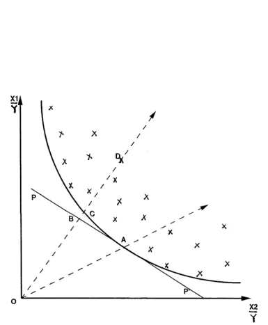
T he above Farrell efficiency measures can be illustrated using Figure 1.1 below. T he u n it-o u tp u t isoquant is represented by the I V curve. All the firms with in p u t-o u tp u t ratios strictly above I V curve, for exam ple, point D, are technically inefficient. T he index of technical efficiency, T E, is defined as the ratio betw een the distance from the origin of th e u n it-o u tp u t isoquant and the distance from th e origin of the given firm ’s norm alized input com bination. W ith reference to Figure 1.1, the index of technical efficiency is defined as

T E OC

O D '

Allocative efficiency is defined with reference to the u n it-o u tp u t isocost repre sented by th e P P ' line in Figure 1.1. A point on th a t line, such as B, represents an in p u t-o u tp u t com bination th a t is efficient from an allocative view point bu t not from a technical one. T he point A is both technically and allocatively efficient. T he index of allocative efficiency, A E, is defined as

A E OB

O C

(15)

~

<

l

>

<

Y

[image:15.550.82.468.130.598.2]

(16)

CHAPTER 1. PRODUCTION EFFICIENCY: AN OVERVIEW 6 and allocative efficiencies, th a t is,

E E T E x AE OC OB CÜD X OC

OB ÖD'

In th a t paper, Farrell proposed to m easure the efficiency of a sample of firms through a set of assum ptions th a t could be im plem ented by linear program m ing (LP) techniques. Consider for exam ple a group of N firms whose efficiency indexes are to be com puted. In the Farrell procedure, the input quantities of each firm, norm alized by the corresponding o u tp u t, form the technical coefficients in a series of N linear program m ing models. The coefficients of the objective functions are th e u n it-o u tp u t quantities produced by each firm. The constraints of the N LP problem s are given by th e norm alized input quantities of each firm m em ber of th e group. T hus, to com pute th e efficiency indexes of N firms, we m ust solve N d istinct linear program m ing problems.

To illu strate th e procedure in greater detail, let us consider three firms th a t produce th e sam e o u tp u t, Y, by m eans of two inputs, X\ and X 2. The m atrix, say, A, of th e th ree LP problem s is constructed as

*11 Yi

* 1 2

y2

* 1 3

Vs

or

a n « 1 2 « 1 3

* 2 1

Vi

* 2 2

v 2

* 2 3

V3 _ a 2i 0 2 2 « 2 3

where th e second subscript identifies the firm and aki = Xki/Yi, k = 1, 2 and i = 1 ,2 ,3 . Now, th e ith LP prim al problem is specified as2

Maximize

Vi — V\ + V 2 + ^3

subject to

a \ \ v \ T « 1 2 ^ 2 T a 13v 3 ^ « l i

(17)

CHAPTER 1. PRODUCTION EFFICIENCY: AN OVERVIEW

a 2 l V l 4" <^22v 2 + 0 2 3 ^ 3 ^ &2i Vj > 0 ; j = 1, 2, 3.

The variable vj represents the output quantity producible by the jth firm

given the output availabilities of the zth firm. The rationale of the Farrell method

exploits the fact that the input quantities of the zth firm produce, by construction,

a unit-output isoquant. Suppose i = 1. Then, if the production process used by

firm number 1 is technically efficient, the solution of the above LP problem will

be V\ = 1, v2 = Vs = 0. Hence, the maximum value of the objective function is

Vj = 1. On the contrary, if both firms number 2 and number 3 are technically

more efficient than firm number 1, the LP solution will be v\ = 0 and v2A v3 > 1, with Vj > 1. This latter case corresponds to the situation where, combining

the technical processes of firms number 2 and 3 with the input availabilities of

firm number 1, it is possible to produce a level of output greater than the unity

quantity. A convenient index of technical efficiency for the zth firm can then be

defined as

T = k*

(b ) O th e r n o n -p a r a m e tr ic p r o g r a m m in g m e th o d s

Since Farrell’s paper, there have occurred some major developments in the

literature for measuring production efficiency in a non-parametric way. Johansen

(1972) developed a linear programming approach with the main aim of deriving

an industry production frontier from the input-output data of individual firms.

Thus he introduced explicitly the notions of a statistical distribution of the input

coefficients when plants are used at full capacity and of a capacity utilization

function. He derived the mathematical conditions under which the aggregate

production frontier will have some conventional functional forms such as Cobb-

(18)

C H APT ER 1. PRODUCTION EFFICIENCY: A N OVERVIEW 8 Johansen is in relating his efficiency concept to (i) short- versus long-run produc tion, (ii) technological change through factor-augm enting processes and (iii) the dynam ics of th e macro-economic process of growth in the tradition of neoclassical models of growth. Johansen’s approach to efficiency m easurem ent has three basic differences from th e Farrell approach. First, it starts from given distributions of capacity am ongst a set of firms and solves for optim al outputs. Secondly, it uses a rule of aggregation to derive the aggregate production frontiers. Thirdly, the micro frontiers derived from th e LP models need not necessarily lead to linear m acro frontiers because of the probability distribution of capacity among the m i cro units. A num ber of authors have followed up this line of work including, for exam ple, Sato (1975), Seierstad (1982), Fprsund and Jansen (1985), Lau and Ma

(1994), am ongst others.

The second m ajor developm ent is the a tte m p t to apply a non-param etric m ethod for testing w hether a finite body of in p u t-o u tp u t d ata (or, in some cases price-quantity d ata) is consistent w ith optim al production (or profit) behaviour. The usual approach is to associate a production function with a given input- o u tp u t d a ta set subject to the lim itation th a t the production function has some specified economic properties, for exam ple, quasi-concavity, m onotonicity and th a t it is efficient in th e sense of a production frontier. This line of economic consistency tests has also been followed up by some authors (see, for exam ple, Hanoch and R othchild, 1972; Diewert and Parkan, 1983; Varian, 1984).

(19)

and/or quasi-market or non-market agencies, for example, public schools, recruit

ment and training programs in defence industries, hospitals, extension services

and family planning programs, where price data are mostly unavailable and there

are multiple goals pursued. The DEA proceeds by constructing a convex hull3 of

the observed input-output observations for a given set of firms, under different

assumptions about free disposability and returns to scale. The DEA problems

may be formulated in output-maximizing or input-minimizing variants and each

DEA problem, however formulated, has a dual. The approach has provided in

recent times a very active field of research for many authors (see, for example,

Sengupta and Sfeir, 1986; Banker and Maindiratta, 1986; Rangan et al., 1988;

Charnes et al., 1990; Aly et al., 1990; Berg et al., 1991; Sueyoshi, 1992; Drake

and Weyman-Jones, 1992; Fukuyama, 1993; Johnes and Johnes, 1993; Fare et

al., 1985, 1994).

M e r its an d d e m e r its o f th e n o n -p a r a m e tr ic p ro g ra m m in g app roach

In general, the non-parametric programming approach is not based on any

explicit model of the frontier. Thus, the principal advantage of the approach

is that no functional form is imposed on the data. It also allows estimation of

frontiers with multiple outputs and multiple inputs. The latter ‘may assume

a variety of forms including those of only ordinal measurements, for example,

psychological tests, arithmetic scores, and so on’ (Charnes et al., 1978, p. 429).

However, the non-parametric approach also has its shortcomings. The Farrell

method, for example, is based on the assumption of constant returns to scale

(CRS) and its extension to variable returns to scale technologies initially proved

(20)

cum bersom e4 (see, for exam ple, Farrell and Fieldhouse, 1962). Secondly, the frontier is com puted from a supporting subset of observations from the sample m aking it particularly susceptible to extrem e observations in the d a ta set. Thus, th e position of the frontier is strongly sensitive to m easurem ent errors. Thirdly, th e efficiency m easures in small samples are sensitive to the difference between th e num ber of firms and the sum of inputs and outp u ts used. This is so because th e sm all num ber of free dimensions rem aining increases the chance of each firm being seen as efficient. Finally, being non-param etric, no statistical inferences on th e estim ates can be carried out. As it will become apparent in the following discussion, th e lim itations of th e program m ing techniques are quite frequently th e strengths of th e statistical approach and the converse is also true.

1.2.2 T h e sta tistic a l approach

For convenience, th e discussion is organized into two parts. The first p art deals w ith production frontier estim ation and technical efficiency m easurem ent using a single cross-sectional d a ta set. The second p art discusses the m easurem ent in th e context of panel d a ta applications.

I Cr o s s-s e c t i o n a l d a t a m o d e l s

D e te r m in is tic fr o n tier s

Let Yi and X{ represent th e o u tp u t and the input vector of th e zth observa tion respectively. T he determ inistic frontier m odel is defined by

Yi = f { X i \ a)exp(—et); i = l , . . . , i V (1.2.1)

4However, the efficiency measure was later on generalized to variable returns to scale (VRS) by F0rsund and Hjalmarsson (1974) and implemented in the DEA formulation by Banker et

al. (1984). Even in the absence of these difficulties, some fundamental problems with Farrell’s

(21)

where a is a vector of unknown parameters; et- is a non-negative term associated

with firm-specific factors which influence the zth firm’s behaviour towards attain

ing maximum efficiency of production; and N represents the number of firms

involved in a cross-sectional survey of the industry. In other words, e,-, is asso

ciated with the technical inefficiency of the firm and implies that exp( — et) has

values which range between zero and one. It therefore follows that the possible

production, is bounded above by the non-stochastic (that is, deterministic)

quantity, /(X,-; a). This is why the model in (1.2.1) is referred to as a deterministic

frontier production function.

Aigner and Chu (1968) first specified (1.2.1) in the context of a Cobb-Douglas

model and suggested that the parameters of the model can be estimated either by

linear or quadratic programming algorithms. However, they did not introduce any

specific form of the distribution of the error term e. Later Schmidt (1976) showed

that if e is exponentially distributed, then Aigner and Chu’s linear programming

procedure is maximum likelihood (ML), while their quadratic programming pro

cedure is ML if e is half-normally distributed. Several other forms of distribution

of e have been used in the literature with corresponding ML estimates, for exam

ple, (i) a two-parameter beta distribution due to Afriat (1972), (ii) one-parameter

gamma distribution due to Richmond (1974), and (iii) a two-parameter gamma

distribution due to Greene (1980a). The choice of any particular distribution of

e, which determines the different ML estimates of a, involves the problem that

the domain of the density of the dependent variable (that is, output Y) depends

on the parameters to be estimated. This violates one of the standard regularity

conditions invoked to prove the general results that ML estimators are consistent

and asymptotically efficient (see, for example, Amemiya, 1973; Barnett, 1976 and

Theil, 1971, p. 392). However, using Wald’s (1949) consistency proof which re

(22)

restrictive sufficient conditions5 on the distribution of e for the ML estimators to

have their consistency property.

As an alternative to ML method, we could apply the method of corrected

ordinary least squares (COLS).6 For example, consider the loglinear case of the

Cobb-Douglas model (1.2.1) and let fi be the mean of e; then we can write

K

ln Y = ( a i - f t ) + ^ 2 a khiXk - ( e - f i ) (1.2.2)

k=2

where the new error term (e — fi) satifies all the standard OLS conditions. Hence,

this equation may now be estimated by the OLS method to obtain best linear

unbiased estimates of (aq — ft) and the a ks. When any specific distribution, for

example beta or gamma, is assumed for e, then we can estimate the parameters

in (1.2.2) from the moments of the distribution of the OLS residuals. Since fi is

a function of these parameters, it too can be used to ‘correct’ the OLS constant

term, which is a consistent estimate of (aq — fi). But this type of ‘correction’

may not always yield non-negative values for all residuals (e — /r) in empirical

applications, thus failing to satisfy the frontier hypothesis of efficiency. One

remedy is to adopt the deterministic approach developed by Greene (1980a). In

this approach, a particular production function is first estimated by OLS. Then,

we correct the constant term by shifting it up until no residual is positive and one

is zero. This provides a frontier with respect to which the technical efficiency of

each firm can be evaluated by measuring the relative distance between the frontier

output and the actual output, given a certain level of input set. A second remedy

is to apply a ‘composed error’ or stochastic frontier model discussed below.

The technical efficiency denoted by, say, TE, of a given firm is defined to

be the ratio of the observed actual output of the firm to its corresponding fron

tier output. Given the deterministic frontier model (1.2.1), the frontier output

5The conditions rule out the exponential and half-normal but permits the log-normal and the gamma densities and, in particular, Greene recommended the latter.

(23)

CHAPTER 1. PRODUCTION EFFICIENCY: AN OVERVIEW 13 denoted by Y*, for the zth firm is

Y- = /(* ,;« )

since in this case, e; = 0. The technical efficiency for the ith firm is then given as

TE, = Y i/Y ’

f( X i ; a ) e x p ( - e j) f ( X a a )

= exp(-ej). (1.2.3)

Thus, in th e context of determ inistic frontiers, the technical efficiencies are esti m ated by obtaining the ratio of th e observed o u tp u t to the corresponding esti m ated frontier o u tp u t, th a t is,

TEi Yi

T he use of determ inistic frontiers for m easuring technical efficiencies has

so m e s h o rtc o m in g s w h ic h in c lu d e :

(i) T he notion of a determ inistic frontier shared by all firms ignores th e very real possibility th a t a firm ’s perform ance may be affected by factors en tirely outside its control (such as bad w eather, m achine or input supply breakdow n, industrial action, and so forth), as well as by factors under its control (inefficiency). To lum p th e effects of the exogenous shocks together w ith effects of m easurem ent error and inefficiency into a single one-sided error term , and label th e m ixture ‘technical inefficiency’ is som ewhat ques tionable. Moreover, this conclusion is reinforced if one considers also the statistical ‘noise’ th a t every em pirical relationship contains.

(24)

CHAPTER 1. PRODUCTION EFFICIENCY: AN OVERVIEW 14 These argum ents lie behind the introduction of stochastic frontier (also called ‘composed e rro r’) m odel of Aigner et al. (1977) and Meeusen and van den Broeck (1977). The essential idea behind the stochastic frontier model is th a t the error term is composed of two parts. A sym m etric com ponent perm its random vari ation of the frontier across firms and captures the effects of m easurem ent error, statistical noise, and other random shocks outside the firm ’s control. A one-sided com ponent captures th e effects of inefficiency relative to the stochastic frontier. In a stochastic frontier therefore, given quantities of a set of inputs, there is a m axim um o u tp u t th a t is possible, but this m axim um level is random rath er th an determ inistic. T h a t is, th e stochastic frontier expresses m axim um o u tp u t, given some set of inputs, as a distribution rath er th an a point.

S to c h a s tic fro n tiers

T he stochastic frontier m odel is defined as

Yi = f ( X l ; a) e xp( e i - et); z = 1 , . . . , TV (1.2.4)

where e, is th e usual sym m etric noise associated w ith random factors not un der th e control of th e firms, while the one-sided error e; w ith e, > 0, captures technical inefficiency relative to th e stochastic frontier. In fact, the effects of th e form er were first recognized by T im m er (1971). He suggested deleting a cer tain percentage of observations, assum ing they are affected by statistical errors and estim atin g w hat he referred to as probabilistic frontier w ith th e rem aining observations using a linear program m ing technique.

T he stochastic specification in (1.2.4) was independently proposed by Aigner

(25)

of the ets. The latter are assumed to be independently and identically distributed

as, for example, exponential (Meeusen and van den Broeck, 1977), half-normal

(Aigner et a/., 1977), truncated normal (Stevenson, 1980) and gamma (Greene,

1990).

Firm-specific technical efficiency, as before, is defined in terms of the ratio

of the observed output to the corresponding frontier output, conditional on the

levels of inputs used by the firm. Thus, the technical efficiency of firm i in the

context of the stochastic frontier production function (1.2.4) is the same as for

the deterministic frontier model (1.2.1), that is,

TEi = Yi/Y*

/( X t;a)exp(et- - et) /( X l;a)exp(el)

= exp(—1{). (1.2.5)

Although the expressions in (1.2.3) and (1.2.5) for technical efficiency of a

firm associated with the deterministic and stochastic frontier models, respectively,

are the same, it is important to note that they may produce different empirical

values for the same firm. For example, firm i will be judged technically more

efficient relative to the unfavourable conditions associated with its productive ac

tivity (that is, et < 0 in /(Ah; a)exp(e;)) than if its production is judged relative

to the maximum associated with the value of the deterministic function, f (Xi; a).

On the other hand, for favourable conditions (et > 0), firm i would be judged

technically less efficient relative to the stochastic frontier than when judged rel

ative to the deterministic frontier. Moreover, the two frontier specifications in

(1.2.3) and (1.2.5) will also generally have different estimates of the as.

Jondrow et al (1982) and Kalirajan and Flinn (1983) independently sug

gested that e,- associated with the stochastic frontier production function in (1.2.4)

be predicted by the conditional expectation of et, given the value of the random

(26)

cases that the e,-s had half-normal and exponential distributions. However, given

the multiplicative frontier production model (1.2.4), Battese and Coelli (1988)

pointed out that the technical efficiency of the zth firm, T E t = exp( — e,-), is best

predicted by using the conditional expectation of exp( —e,-), given the value of

the random variable, £t = — e;. The latter result was calculated for the more

general stochastic frontier model involving panel data and the Stevenson (1980)

model for the e,s.

The primary advantage of stochastic over deterministic frontier production

functions is that the former allow for technical inefficiency to be measured sep

arately from statistical noise. Employing a stochastic frontier can also be seen

as allowing for some types of specification error and for omitted input variables

uncorrelated with the included inputs. However, obtaining firm-specific estimates

of efficiency is more involved with a stochastic frontier model than with a deter

ministic frontier one, which directly yields estimates of firm-specific inefficiency

terms as the residuals from the estimation (Greene, 1980a). Schmidt and Sickles

(1984) also pointed out other difficulties in applying stochastic frontier produc

tion models using cross-section data. First, because there is only one observation

for each firm and that firm inefficiency is modelled as a firm-specific effect, one

cannot get consistent estimates. Second, separation of inefficiency measures from

statistical noise depends on specific assumptions about the distribution of techni

cal inefficiency. This means that estimation of technical efficiency can be sensitive

to these a priori distributional assumptions. In particular, different distributional

assumptions can lead to substantially different results for the estimated technical

efficiencies. Third, the assumption that the inefficiency term is independent of

the input levels is not realistic since

(27)

II PANEL DATA MODELS

Schmidt and Sickles (1984) detailed three principal benefits of using panel

data in estimating production frontiers and technical efficiency measures. Firstly,

no specific distributional assumptions are necessary for consistent estimation of

the as and the es. Secondly, in the single cross-section estimates, it is assumed

that inefficiency and factor input levels are independent. As note above, this

may be unrealistic. Any correlation between the factor inputs X and the level

of technical inefficiency e will imply that the standard estimates are inappropri

ate. However, panel data models do not necessarily require this independence

assumption (see, for example, the fixed effects model discussed below). Given

the potential correlation between the inputs and inefficiency levels illustrated by

the above quotation, this is clearly an important advantage of estimates based

on panel data over those based on single cross-sections. Finally, in panel data

models, assuming that the inefficiency terms are time-invariant, the random error

component in the ‘composed error’ can be averaged out over time so that what

remains is the required inefficiency component. This cannot be done with the

cross-sectional data model where for each firm we have only one inefficiency term

not T terms as in the panel data case.

(A)

Time-invariant firm effects

For a small number of time points, T, the firm effects can be assumed to vary

across firms but remain constant over time. In such circumstances, the production

frontiers and technical efficiency measures can be estimated as follows:

D e te r m in is tic fro n tiers

Assuming, for example, a Cobb-Douglas specification for the production

function, f ( X a; a), the panel data model in logarithmic form can be written as

(28)

CH AP T E R 1. PRODUCTION EFFICIENCY: A N OVERVIEW 18 i = 1 , . . . , TV and t = 1 , . . . , T

where y and xs are logarithm s of Y and X s respectively and e, > 0 for all i. The estim ation procedure is straightforw ard (see, for exam ple, Greene, 1980a). As in th e cross-sectional case, ordinary least squares (OLS) leads to a consistent estim ato r of a . A consistent estim ator of ou is obtained from the OLS estim ator shifted in order to obtain positive values for the residuals, th a t is,

as, l = aoLS,i + max(ej), (1.2.7)

X

where et are th e OLS residuals from equation (1.2.6), as,\ and cxols,i denote the

shifted intercept and the OLS estim ates respectively. The shifting am ounts to assum ing th a t at least one firm is 100% technically efficient and the efficiency of other firms are m easured relative to it. Thus, the technical efficiency of each observed u n it m ay be obtained as

TEi exp |m a x (e ,) — e , | . (1.2.8)

As previously noted, the lim itation of the determ inistic approach rests in th e fact th a t all th e observations lie on one side of th e frontier; th e procedure is therefore very sensitive to outliers and it does not allow for random shocks around an average production frontier.

S t o c h a s tic fr o n tier s

T he stochastic frontier production function in logarithm ic form is expressed as

Vit = O il + x'ita + £jt; i = 1 and < = 1 , . . . , T (1.2.9)

where

(29)

tit-CHAPTER 1. PRODUCTION EFFICIENCY: AN OVERVIEW 19

The en is a ‘composed error’ term that combines the time-invariant latent individ

ual effects et- and the disturbance terms elt assumed to be normally distributed and

uncorrelated with both et and the explanatory variables in the model. Following

Schmidt and Sickles (1984), we assume that the individual effects e; characterize

the inefficiency of the firms. Furthermore, if we assume that e,- > 0, equation

(1.2.9) corresponds to a special case of the stochastic frontier model introduced

by Aigner et al. (1977) and Meeusen and van den Broeck (1977). The difference

lies in the fact that for the panel data, equation (1.2.9) provides a natural way

to discriminate between the inefficiency indicator and the statistical noise.

In order to be able to apply the main results of the panel data literature, we

first rewrite equation (1.2.9) as

Vit = x'ita + otu + t it (1.2.10)

where

a n = oil — e,.

Now, depending on the assumptions one is willing to make, the as, es and tech

nical efficiency measures can then be estimated by any of the following methods:

(a) F ixed effects m odel and the ‘w ith in ’ estim ators

While the e in (1.2.10) is unobservable by the researcher, its persistence

would lead us to expect firms to observe e and to take its level into account when

choosing their inputs. If so, then the inputs and the es will be correlated. Under

such circumstances, the fixed effects procedure which includes the es (firm-specific

effects) as regressors rather than relegating them to the error term will provide

consistent estimates. The procedure utilizes the panel structure of the data to

control for the firm-specific unobservables by including firm-specific dummies

or by replacing each variable by the deviations of the observations from their

(30)

indicated here by the subscript W, can be obtained by regressing the ‘within1

group deviations of yn on those of xn, that is,7

Vit - Vi. = { X u - X i , ) ' a w + e w , i t (1.2.11)

and

— Vi. ~ x 'i.a W (1.2.12)

where

&W,it — t i t W ,

1 T l T

Vi. = and Xi. = - ^ 2 x it.

1 t = i 1 t = l

Alternatively, the dummy-variable least-squares (DVLS) approach can be

used to estimate the a and a i values where the latter are the parameter estimates

of firm-specific dummy variables. The advantage of DVLS is the ease of obtaining

standard errors for all parameter estimates of the model. However, the DVLS

approach may not be feasible if N is very large since it requires putting in N

dummy variables.

In either case, the fixed effects technique is a ‘within-firnT regression. It

utilizes only the variability of the data within each firm through time and not the

variability of the data across firms at any given point in time. Thus one of the

shortcomings of the method is that it fails to exploit fully the rich information

panel data can provide.

The levels of performance, e^,j, can be obtained on the basis of the estimated

fixed effects etw,u m (1.2.12) by assuming that the most efficient firm in the sample

corresponds to max;(aw,it) and that the inefficiency level is given by the distance

(Schmidt and Sickles, 1984):

e \v ,i = m a x ( d w , i t ) — a \ v , u -X

(31)

Using this estim ated e\v,i, the technical efficiency of the zth firm denoted by, say, TEw,i is then obtained as

(b) R a n d o m e ffe c ts m o d e ls and th e G LS e stim a to r

As long as there is no correlation between the regressors (inputs) and either en or et, the random effects technique, which is ju st GLS applied to equation (1.2.10) will provide consistent and efficient estim ates of the param eters. Unlike the fixed effects m odel, this procedure utilizes variation in th e d a ta both between firms at a given point in tim e as well as w ithin each firm through tim e to estim ate the coefficients. This additional variation gives random effects a significant advantage over fixed effects estim ates when there is no correlation between the regressors and th e es.

In th e random effects m odel, instead of working conditionally on the effects e,, we explicitly take into account th eir stochastic nature. This can be particularly appealing in the framework of estim ating efficiencies since random elem ents may affect th e efficiency of each firm. In this approach, there is a unique production frontier b u t one sided random deviations are allowed in order to characterize inefficiencies.

T he GLS estim ators, indicated by th e subscript G L S, are obtained by per form ing OLS on th e equation8

TEw,i = ex p (—ew,t); i — 1 , . . . , N. (1.2.13)

Vit — Oyi . = { x i t — 0Xi.)'c)LGLS + £ GLS,it (1.2.14)

l 1 , . . . , N and t = 1 , . . . , T

where

6

(32)

and

£g l s,h = (1 — 0)ql\ + (tu — Ot{). (1.2.15)

When (j\ and cr^, the variances of t and e are unknown, they can be estimated,

for instance, by performing OLS on equation (1.2.10) as suggested by Wallace

and Hussain (1969). In this case, the estimator is called the feasible GLS.

In order to estimate technical efficiencies, an estimate of the e; is required.

Following Schmidt and Sickles (1984), the residuals may be recomputed from

equation (1.2.9) with the more efficient GLS estimates of a from (1.2.14). Aver

aging these residuals over time, we get

1 T

£*. = (1.2.16)

1 t= l

The estimates from (1.2.16) are consistent as T —> oo provided ctcLS is consis

tent and the latter requires either N —* oo or be known. Now, since E(ea) = 0

and et- = et< — £,•<, a natural estimate of e;, denoted by ecLS.ii is simply given by

CGLS,i = max(£,.) — (1.2.17)

i

where the maximum is introduced in order to provide positive values of the es.

From (1.2.17), the technical efficiency of the ith firm denoted by say, T Eqls,

is then estimated as

T EglS'I = exp(—e GLS,i)- (1.2.18)

R a n d o m or fix ed e ffe cts m o d els?

As expected, the fixed effects (‘within’ estimators) and random effects (GLS

estimators) models may yield potentially different results. For instance, Kumb-

hakar (1986), in his study of the US class I railroads, found that the estimates of

inefficiency in the fixed effects models are much higher than those of the random

effects models. We, therefore, have to choose the model that most fits the sample

(33)

Traditionally, the way to choose between these two models is to employ

the Hausman test (Hausman, 1978), which measures the distance between the

estimated fixed and random effects coefficients. When there is no correlation

between the regressors and the es, both fixed and random effects techniques yield

consistent estimates of the parameters, so the distance between the estimated

coefficients should be very small as the sample size increases. On the other

hand, when there is correlation between the es and the regressors, the random

effects estimates are inconsistent and hence converge to something different from

the true values of the parameters, that is, the values to which the fixed effects

estimators are converging. Hence, in this case the distance between the fixed and

random effects estimates should be relatively large, resulting in a large value of

the Hausman test statistic.

In summary, if there is no correlation between the regressors (inputs) and

the es, the random effects specification is most efficient and is therefore to be

preferred. On the other hand, if there is correlation between the regressors and

the es, the fixed effects specification is theoretically superior because it can still

provide consistent estimates. At the same time, one should view the fixed effects

estimates with caution. If the regressors are almost time-invariant, it may lead

to multicollinear regressors in equation (1.2.10). The fixed effects specifications

may, therefore, produce a poor estimation of the intercepts and of the slopes of

the production frontiers and so, unreasonable measures of efficiency (see, for ex

ample, Simar, 1992). Moreover, such time-invariant regressors can sometimes be

eliminated in the ‘within’ transformation. In this case, the estimated individual

effects will include the effects of all variables that are time-invariant but not in

any sense a representation of inefficiency. This would make inefficiency compar

isons difficult unless the excluded time-invariant variables affect all firms equally.

In fact these latter problems may be so great that the random effects specification

(34)

the regressors and the es.

(c) M axim um likelihood estim ation (MLE)

To estimate the model in (1.2.9) by maximum likelihood method, distribu

tional assumptions for e,- and ta are required. Pitt and Lee (1981) first developed

MLE techniques using panel data to estimate frontier production functions and

mean technical efficiency measures based on the following assumptions:9

(i) The tu are independent and identically distributed as jV(0,of). The com

ponent e,- is independent and identically distributed one-sided, non-negative

error, which is derived from a N (0, aj) distribution truncated from below.10

(ii) e,; is independent of e,t as well as of the input variables included in the

model.

Writing a stochastic frontier production function in a panel data context as

Yit = f{Xa; a)exp(e,* — et) (1.2.19)

i = 1 , . . . , N and t = 1 ,..., T

where Yu and Xu are the output and input vectors for the zth firm at the tth time

period, respectively, P itt and Lee (1981) showed that the joint density function

of the composed error £,* = tu — et- denoted by say, </>(e), can be derived from the

convolution formula:

roo 1

^(^ti i • • • i £jt) — / I I T e,)/i(e,)dei, (1.2.20)

J o t =i

where g ( t i t ) is the density function of t a and

h(ei) 5 e t- > 0 . (1.2.21)

9Pitt and Lee (1981) considered three versions, models I, II and III. This discussion refers to model I.

(35)

CH AP TE R 1. PRODUCTION EFFICIENCY: A N OVER VIEW 25 Assuming independence across firms, the likelihood function for the pooled d ata is

N

L = <f>{en, • • • ,£ tr)- (1.2.22) i=i

The MLE estim ates of a denoted by olmle can be obtained by m aximizing (1.2.22) or its logarithm .

W ith the specification (1.2.19), a m easure of each u n it’s technical efficiency can be defined as

T E it Yit

f ( X lt‘a)exp(eit)

e x p ( - e t) (1.2.23)

for th e T h firm in th e tth tim e period.

For th e individual firm-specific inefficiency term , e,- in (1.2.23), B attese and Coelli (1988) suggested th a t it can be predicted as11

e,- = m; + - ^ ( - M ' / c r , ) ] - 1} (1.2.24)

where

M* = + r - V e2]K 2 + r - y 2) - \ (1.2.25)

^.2 = <7

y,tf

+ T o * ) - \ (1.2.26)

£i. =

t=1

and $ is stan d ard norm al cum ulative distribution function.

(1.2.27)

Using (1.2.24) above, B attese and Coelli (1988) proposed a m easure of firm- specific technical efficiency, denoted here by T Eßc,i-, as

T Eßc,i exp ( —et)

f 1 - $[<r. - (M,*/cr.))}

I

1 - $( —M*/cr.) / exp (—M* + (1.2.28)

(36)

(B)

Time-varying firm effects

Application of the model based on the assumption of time-invariant firm

efficiency has been criticized in several cases, particularly in relation to studies

involving panel data with sufficiently many time points. Economists argue that

it is not possible for firms to be unaware of their inefficiency, if the period of

investigation is sufficiently long. If inefficiency is detected, then it would be eco

nomically irrational and unrealistic for a profit-maximising decision-maker not to

respond to it. Therefore, the time-invariance assumption of technical efficiencies

over time without formally testing its appropriateness may result in inconsistent

estimates of the parameters of the model as well as misleading conclusions about

technical efficiency.

In order to relax the time-invariance assumption while retaining the advan

tages of panel data, Cornwell et al. (1990) developed an approach that imposes

some structure on how inefficiency varies over time. In their model, the firm-

specific effects are expressed as a function of time with the intercept terms as

well as the slope coefficients12 (of the time variable) varying across firms. Basi

cally, they generalize Schmidt and Sickles (1984) by replacing the firm effects, e,-*,

by

tu = I n + 7»‘2* + 7i3*2; * = l , . . . , i V and t = 1 , . . . , T. (1.2.29)

This specification allows the inefficiency terms to vary over time as well as across

firms. The Cornwell et al. model can be estimated by the ‘within’, GLS, MLE

or Hausman and Taylor (1981) instrumental variable (IV) methods, depending

on the assumptions the researcher is willing to make about the independence and

the distribution of the firm-specific effects.

Kumbhakar (1990) started with an equation similar to (1.2.9), but proposed

(37)

C H A P T E R 1. PRODUCTION EFFICIENCY: A N OVERVIEW’ 27 th e following form ulation for ett:

ett =

C ( 0 C*'»

t = and z = l , . . . , i V (1.2.30) where

C ( 0

1 + exp(6£ + ct2) , (1.2.31) in which b and c are coefficients to be estim ated. The resulting system is estim ated by MLE m ethod.

B attese and Coelli (1992) suggested a tim e-varying firm effects model for unbalanced panel d a ta (the balanced one being a special case), such th a t the technical efficiencies of firms either m onotonically increased or decreased or re m ained constant over tim e. They defined elt as

eit - {exp[—t/(£ — T’)]}e,, t £ I(z ); z = l , . . . , J V ; (1.2.32) where th e ets are assum ed to be independent and identically distributed non negative tru n catio n s of th e N(fi, <r2) distribution; rj is an unknown scalar param  eter; and l ( i ) represents th e set of Ti tim e periods among the T periods involved for which observations for th e zth firm are obtained.13

B attese and Coelli (1992) also showed th a t th e m inim um m ean squared error predictor of th e technical efficiency of the zth firm at the tth tim e period, T E lt = exp (-C jt), is

-®[exp(—e*t|£t)]

1

1 J

exp + ^ ta l t .(1.2.33)

T he e, represents th e (Tt x 1) vector of eas associated w ith th e tim e periods observed for th e zth firm where sa = tu — et<;

II

* •

*»

o-2 + r j \ r \ x a l

n-2

-a * i —

(38)

T)i represents the (Tt- x 1 ) vector of r]lts associated with the tim e periods observed for th e ith firm; represents the d istribution function for the standard normal random variable; aj and cr\ are variances of e,* and respectively.

The exponential specification of th e firm effects in (1.2.32) over tim e is a som ew hat rigid param eterization in th a t technical efficiencies estim ated from th em m ust either increase at a decreasing rate (77 > 0 ), decrease at an increas ing rate (77 < 0) or rem ain constant (77 = 0). To perm it greater flexibility in th e n atu re of technical efficiency variation over tim e, B attese and Coelli (1992) suggested an altern ativ e tw o-param eter specification defined as

e,f = {exp[l + t7!(* - T) + r}2{t - T ) 2]}et (1.2.36) where 77! and 772 are unknown param eters. This model perm its firm effects to be convex or concave and the tim e-invariant model being a special case in which

V i = rj2 = 0.

P r o b le m s w it h t h e M L E p r o c e d u r e s

A lthough the superiority of the MLE is undisputed if the sam pling d istri butions of th e errors are correct, when used in th e context of technical efficiency m easurem ent, it still a ttra c ts some criticism s which include th e following:

(i) E stim ations are carried out under th e assum ption of no correlation between th e individual-specific inefficiency term s and the input levels. This may be an unrealistic assum ption especially in a panel d ata context. As noted above, if th e period of investigation is sufficiently long, firms m ay be able to detect th eir inefficiency and are likely to respond, for exam ple, by adjusting th eir in p u t levels. In such circum stances, th e inefficiency term s and the input levels m ay be correlated.

(39)

(the inefficiency term ). Severe assum ptions are often made, including the restriction th a t the mass of the inefficiency density is most concentrated at zero. The sensitivity of the efficiency estim ates to assum ptions makes com parisons of th e results from different studies problem atic.

(iii) In general, the choice of specific inefficiency distributions should ideally be based on th e economic mechanisms generating cross-section inefficiency differences. W hen such inform ation is lacking, the choice of specifying a particu lar d istribution and then applying m axim um likelihood is som ewhat arbitrary.

In each of th e estim ation m ethods discussed above, we briefly m ade some com m ents on th eir suitability, shortcom ings a n d /o r how realistic are the assum p tions on which they are based. We now tu rn to some of th e criticism s th a t are generally levelled against both th e program m ing and statistical approaches to technical efficiency m easurem ent. We also look at some recent developm ents th a t have taken place m ainly in response to some of these criticisms.

1.3 P r o g r a m m in g a n d s ta t is t ic a l a p p ro a ch es:

S o m e c r itic is m s a n d e x te n s io n s

(40)

CHAPTER 1. PRODUCTION EFFICIENCY: AN OVERVIEW 30 1 .3 .1 T h e n o n -p a r a m e tr ic p r o g r a m m in g a p p r o a ch

In section 1.2.1, we noted th a t m ajor criticism s of the program m ing ap proach are th a t being non-param etric, the constructed production frontiers have no statistical properties to be evaluated upon and th a t the approach attrib u tes all deviations from th e frontier to inefficiency w ithout accounting for random in fluences or statistical errors. Moreover, since th e frontier is constructed from the supporting subset of observations from the sam ple, it is particularly susceptible to extrem e observations and m easurem ent errors.

However, there have been various a tte m p ts to combine the flexibility of the production frontier representation of the non-param etric approach w ith th e abil ity of handling statistical errors. First, Varian (1985) introduced stochastic char acteristics into th e program m ing approach by introducing two-sided deviations to incorporate th e random noise and to calculate the efficiency m easures free of such m easurem ent errors. Second, Land et al. (1989) suggested the chance-constrained program m ing techniques to allow for uncertainty about the stru ctu re of th e effi cient production technology. However, d ata requirem ents for this type of analysis are m ore dem anding, because besides th e in p u t-o u tp u t d ata, chance-constrained analysis requires inform ation on th e accuracy of d a ta and willingness to under take risk. Furtherm ore, chance-constrained efficiency m easurem ent continues to be determ inistic. Efficiency is calculated by m eans of nonlinear program m ing techniques and no param eters are actually estim ated in the process.

(41)

M inim al functional constraints are imposed as in the DEA and at the same tim e, a com posed-error specification is borrowed from the statistical approach to frontier estim ation. However, the com bination of the advantages of both program m ing and statistical approaches comes at the cost of some analytical com plexity in the derivation of the likelihood equations involved.

Fourth, Banker (1993) provided a formal statistical basis for the efficiency evaluation techniques of the DEA. The DEA estim ators of the frontier production function, assum ed m onotone increasing and concave, are shown to be m axim um likelihood estim ators if th e deviation of actual o u tp u t from the efficient o u tp u t is regarded as a stochastic variable w ith a m onotone decreasing probability density function. The estim ators also exhibit the desirable asym ptotic property of con sistency, and th e asym ptotic distribution of th e DEA estim ators of inefficiency deviations is identical to the tru e distribution of these deviations. Banker then employed this result to suggest possible statistical tests of hypotheses based on asym ptotic distributions.

(42)

1 .3 .2 T h e s t a t i s t i c a l a p p r o a c h

Progress towards eliminating criticisms levelled against the statistical ap

proach to measuring production efficiencies has been relatively slow. In his recent

survey, Bauer (1990a, p. 41) remarked

. . . the basic set of econometric estimation techniques has changed rela tively little in recent years . . .

And van den Broeck et al. (1994, p. 274) added that

. . . the entire literature has been embedded in the sampling theory paradigm.

In addition to the estimation problems and restrictive assumptions underlying

the various procedures discussed in section 1.2.2, there are two major criticisms

that are levelled against the statistical approach in general.

(a) S a m p lin g d is tr ib u tio n a l a ssu m p tio n s