Tikhonov Regularization as a Complexity Measure in Multiobjective Genetic Programming

Multiobjective Genetic Programming

.

White Rose Research Online URL for this paper:

http://eprints.whiterose.ac.uk/85545/

Version: Accepted Version

Article:

Ni, J. and Rockett, P.I. (2014) Tikhonov Regularization as a Complexity Measure in

Multiobjective Genetic Programming. IEEE Transactions on Evolutionary Computation, 19

(2). 157 - 166. ISSN 1089-778X

https://doi.org/10.1109/TEVC.2014.2306994

(c) 2014 IEEE. Personal use of this material is permitted. Permission from IEEE must be

obtained for all other users, including reprinting/ republishing this material for advertising or

promotional purposes, creating new collective works for resale or redistribution to servers

or lists, or reuse of any copyrighted components of this work in other works

[email protected] https://eprints.whiterose.ac.uk/

Reuse

Unless indicated otherwise, fulltext items are protected by copyright with all rights reserved. The copyright exception in section 29 of the Copyright, Designs and Patents Act 1988 allows the making of a single copy solely for the purpose of non-commercial research or private study within the limits of fair dealing. The publisher or other rights-holder may allow further reproduction and re-use of this version - refer to the White Rose Research Online record for this item. Where records identify the publisher as the copyright holder, users can verify any specific terms of use on the publisher’s website.

Takedown

If you consider content in White Rose Research Online to be in breach of UK law, please notify us by

(will be inserted by the editor)

Training Genetic Programming Classifiers by Vicinal-Risk

Minimization

Ji Ni _· Peter Rockett

Received: May 13, 2014/ Accepted: ???

Abstract We propose and motivate the use of vicinal-risk minimization (VRM) for training genetic programming classifiers. We demonstrate that VRM has a number of attractive properties and demonstrate that it has a better correlation with gener-alization error compared to empirical risk minimization so is more likely to lead to better generalization performance, in general. From the results of statistical tests over a range of real and synthetic datasets, we further demonstrate that VRM yields consistently superior generalization errors compared to conventional empirical risk minimization.

Keywords Genetic programming·Classification·Vicinal-risk minimization

1 Introduction

Classification [8] is one of the most important tasks in machine learning and aims to discover a discriminating function that maps anN-dimensional input vector,x_∈RN

to a label,y_{∈ {−}1,+1}; without loss of generality we consider only binary, or two-class, classification in this paper. Empirical learning is ill-posed [4, 25], which means that classifiers trained by minimizing the empirical risk (i.e, the fraction of misclas-sified training patterns) can exhibit a range of generalization errors over unseen test data. This ill-posedness is particularly acute for small datasets; it is the case of small datasets that weexplicitlyaddress in this paper. For some given size of training set, there is a trade-off between the empirical risk and the complexity of the discrimi-nating function [4]. Overly simple functions lack sufficient flexibility to capture the

J. Ni

Department of Electronic and Electrical Engineering, University of Sheffield, Mappin Street, Sheffield, S1 3JD, UK

E-mail: [email protected]

P. Rockett

Department of Electronic and Electrical Engineering, University of Sheffield, Mappin Street, Sheffield, S1 3JD, UK

class concepts, have a large training error and underfit. At the other extreme, overly complex functions produce decision surfaces with low – possibly zero – training error but which overfit the training set. Both extremes – underfitting and overfitting – yield large generalization errors over independent test data. In general, there exists some ‘optimal’ model complexity between underfitting and overfitting although addressing thismodel selectionproblem is often challenging. One of the great strengths of ge-netic programming (GP) for the empirical modeling of data is that the complexity of the function can evolve to match the data at hand. Nonetheless, the loss function on which a GP classifier is trained plays a pivotal role.

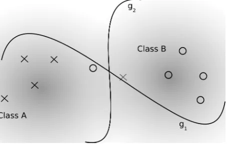
A straightforward illustration of the deficiencies of empirical risk minimization (ERM) is shown in Figure 1 where a small training set of non-separable data is as-sumed drawn from two, arbitrary, two-dimensional class distributions, also shown. The training data are separated by two arbitrary candidate decision surfaces,g1and g2.

Fig. 1 Illustration of the deficiency of 0/1 loss. A small training set, shown as crosses and circles have been drawn from the distributions of class A and B, respectively.g1andg2are two arbitrary, candidate

decision surfaces.

As gauged by the empirical risk, g1andg2give identical values because both misclassify two training set patterns out of ten. There is no reason to prefer one deci-sion surface over another; more generally,anyfunction which misclassifiesanytwo training patterns cannot be set apart fromg1andg2by ERM. As to the generalization abilities ofg1andg2, it is clear thatg1will exhibit a worse test error thang2since it does a worse job of separating the two underlying class distributions although this, of course, cannot be judged by ERM over this training set. Note that this problem is nothing to do with under- or overfitting, but rather, a fundamental limitation of em-pirical risk. In summary, it is clear that the same value of emem-pirical risk can produce a range of possible generalization errors – it is, of course, the objective of machine learning to produce the best possible generalization error. It is noteworthy that almost all GP classifiers reported in the literature have involved minimizing empirical risk.

ma-chine learning field. Classically,regularization[24] seeks to minimize the weighted sum of a risk functional and some measure of discriminant complexity although how to decide on the weighting (the so-called regularization constant) between the two terms usually involves cross-validation [4]. The parsimony principle [18] much-used in GP is an example of regularization. Minimum description length (MDL) ap-proaches [20] can also be viewed as regularization. Iba et al. [13] attempted to apply MDL to GP but failed to account for the not-necessarily-minimal form of the trees – logically, MDL can only be applied to trees which have been simplified to truly minimal algebraic form which, we suspect, is an NP-complete task. In Bayesian ap-proaches, the log prior can be interpreted as a regularization term [25].

Over the past twenty years, the structural risk minimization (SRM) framework of Vapnik [25] has been a dominant paradigm in machine learning and has lead to the powerful notion of maximum margin classification as well as support-vector ma-chines (SVMs). Application of SRM to genetic programming classifiers, however, is technically difficult. Borges et al. [2] interpreted the number of multiplication and division nodes in GP trees as the Vapnik-Chervonenkis (VC) dimension of their dis-criminant function and claimed to apply SRM principles to GP training although they offered no theoretical justification as to why this quantity is connected to the shatter-ing dimension [4] of the function. The fact that these authors were able to observe improved performance was probably because their “VC dimension” was employed in a conventional regularization framework and the value of the regularization con-stant tuned to yield improved performance over non-regularized comparators. Amil et al. [1] derived an expression for the VC dimension of a GP tree proportional to the upper bound on the number of nodes in the tree (assuming no exponential function nodes) although the tightness of this bound, and therefore its adequacy for SRM, is unknown [11].

Exploring the complexity of the discriminant implemented by a GP tree is feasi-ble using multiobjective (MO) [27] (or other parsimony) methods by simultaneously minimizing the empirical error/complexity leading to a (Pareto) set of solutions which delineate this trade-off. The problem remains, as we have argued above, that minimiz-ing the empirical risk over a trainminimiz-ing set does not necessarily equate to minimizminimiz-ing the generalization error of the resulting classifier. The fact that the empirical risk over a training-set is a one-to-many mapping to test error undermines the validity of the regularization framework, especially under the small sample conditions that we are expressly addressing here. For this reason we have explored the use of an improved loss function for training GP classifiers.

2 Vicinal Risk

Given some set ofℓtraining data drawn independent and identically-distributed (iid) from a data distributionP(x,y):

D_={x1→y1,x2→y2, . . .xℓ→yℓ}

wherexi∈RN andy∈ {−1,+1}, the task of training ascoringclassifier in machine

learning is to select some discriminative function f(x)such that:

f(x)

(

<0 Predict class ‘-1’

≥0 Predict class ‘+1’ (1)

We require to select the f(x)which minimizes the expected risk,R(f)which will ensure optimum generalization over future unseen examples drawn fromP(x,y):

R(f) =

Z

L[f(x),y]dP(x,y) (2)

whereLis some loss function. Unfortunately,P(x,y)is not known in practice and so a conventional approximation has been to minimize theempiricalrisk,Remp(i.e., the

expectation of 0/1 loss) over the training set. We take the loss function to be:

L[f(x),y] =H[−y f(x)] (3)

whereH()is the Heaviside step function. Thus forx-values which would give rise to a misclassification, (3) is unity; conversely, forx-values which yield correct classifi-cation, the loss is zero. ThusRempcan be formally defined as:

Remp(f) =

1

ℓ

ℓ

∑

i=1

H[−yif(xi)] (4)

As is clear from the above, the fundamental shortcoming of the 0/1 loss is due to its discrete nature, in particular, that a pattern is either classified correctly, in which case it contributes zero to the cumulative loss, or the pattern is misclassified and so contributes unity to the loss. Crucially, no account is taken of themarginby which a pattern is misclassified (or indeed, correctly classified). A misclassified pattern which is just the wrong side of a decision surface is weighted equally with a pattern that is a very large distance from the decision surface; intuitively, the latter case should be treated as more serious than the former. As a logical consequence, a pattern’s distance from the decision surface should weight its contribution to the loss1.

Vapnik [25] has motivatedvicinal riskby assuming that the (unknown) data dis-tribution is locally ‘smooth’ in which caseP(x,y)can be approximated by placing avicinity functionon each training datum – this process can be thought of as either resampling or, equivalently, interpolatingD_{. Since the shortcomings of 0/1 loss are}

due to its discrete nature, smoothing the training set will have the effect of stabilizing the training process. Vapnik [25] described two possible types of vicinity functions,

hardandsoft. Hard vicinity functions have an abrupt cutoff at some distance from a training datum – under a 2-norm, this would be a ball or hypersphere centered on each datum. Whereas a hard vicinity function has a constant, non-zero value up to the cutoff distance and zero beyond, a soft vicinity function, such as a Gaussian kernel, typically has a peak value at the training datum and a monotonically-reducing value with increasing distance from the datum. Entirely equivalently, placing a kernel over each training datum can be viewed as approximatingP(x,y)using a Parzen windows density estimator [3, 8] for which a Gaussian kernel is a natural choice2_{. Here we} develop the soft vicinity function approach because: i) it is more tolerant of the set-ting of scale of the kernel and ii) there is a technical requirement with hard vicinity functions that they do not overlap in pattern space [25].

Taking the loss function given in (3), analogous to minimizing (2), we wish to select the fwhich minimizes the vicinal risk,RVRwhich is the expectation of (3) over the data distribution. Writing the necessary risk functional in a somewhat different form to Vapnik:

RVR(f) =

Z

L[f(x),y]dP(x,y) (5)

≈1_ℓ

ℓ

∑

i=1

Z

H[−yif(x)]G(x|xi,σi2)dx (6)

whereG()is the Gaussian kernel of varianceσ2

i placed on thei-th datum, andP(x,y)

is approximated by the Parzen windows estimate of a sum of Gaussians. The inte-gral within (6) has a straightforward interpretation as the hypervolume, in the N-dimensional pattern space, of the portion of thei-th kernel which falls on the ‘wrong’ side of the decision surface and hence would give rise to misclassification.

A number of properties of VRM is apparent:

– Under VRM, we seek to minimize a continuous function (6), thereby removing the problem with 0/1 loss of being discrete. Patterns contribute to the loss depend-ing on their distance from the decision surface, or more strictly, the hypervolume of the kernel function falling on the ‘wrong’ side of the decision surface. It is clear that correctly-classified patterns a long way from the decision surface will make a very small contribution to the loss and will hence have a minimal influence on the placement of the decision surface – this is highly desirable since only data in the vicinity of the decision surface run the risk of misclassification and should ‘negotiate’ the location of the decision surface.

– At distances greater than≃3σ_{from the decision surface, the contribution to the}

loss of an incorrectly-labeled datum saturates at unity, conferring robustness to outliers.

– Asσ2_{→0, the Gaussian kernel in (6) tends to aδ-function and so the vicinal} risk tends to the empirical risk in (4). Thus empirical risk can be understood as a special case of vicinal risk.

2 _{We omit the normalization of the Parzen density estimate since this contributes only a multiplicative}

– Asσ2_{→∞, the value of risk (6) tends to 0.5 since in the limit, ‘half’ the kernel} extends either side of the decision surface.

– σ2_{defines a characteristic ‘scale’ for the learning problem which will vary by} dataset.

Chapelle et al. [3] have directly minimized VRM for linear classifiers, assign-ing each trainassign-ing datum kernel its own value ofσ2

i proportional to a measure of

local density although the constant of proportionality had to be determined by cross-validation. As far as we are aware, the present paper is the first report of applying VRM to genetic programming classifiers.

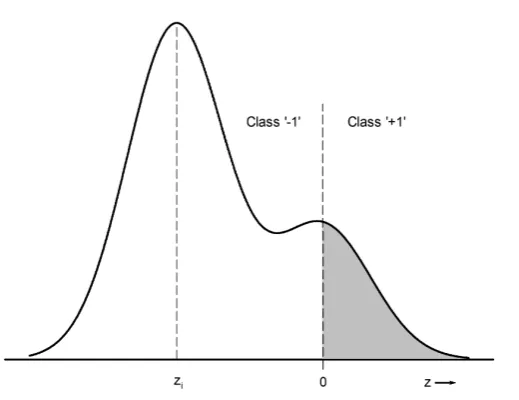
Key to the computational tractability of VRM in genetic programming is the evaluation of the integral in (6). Rather than the inconvenient evaluation of an N-dimensional integral, we can propagate the Gaussian kernel on thei-th pattern through into the 1D decision space, the image of f(x). This yields a distributionpi(z)in the

1D decision space,zas shown in Figure 2. Notice that because the mapping imple-mented by a GP tree will, in general, be non-linear, pi(z)will be not generally be

a Gaussian distribution despite the samples being Gaussian-distributed about xi in

pattern space. Equation (6) for the vicinal risk can be rewritten as:

RVR≈ 1

ℓ

ℓ

∑

i=1

Z

H[−yi×z]pi(z)dz (7)

Notice that the integrals under the summations in both (6) and (7) evaluate the probability of a point drawn fromG(x_|xi,σi2)being misclassified. To approximate

the integral in (7) we can conveniently use Monte Carlo integration [21] whereby for thei-th pattern, we drawqi samples from the Gaussian distributionG(x|xi,σi2),

and propagate each resulting vector through f to yield a corresponding set of scalar values of z. Counting the number of values of zwhich predict the incorrect class according to (1) for the i-th training pattern, and dividing by qi approximates the

value of the integral for thei-th pattern in (7); evaluating an integral by Monte Carlo in 1D is much more efficient than performing the same evaluation inNdimensions, particularly whenN is large [21]. The probability of misclassification for thei-th pattern is illustrated by the shaded region in Figure 2. It is the expectation of this probability over the training set that we seek to minimize which is achieved by taking the expectation over the integrals (i.e. averaging) in (7).

We can conveniently organize the Monte Carlo integration and the calculation of (7) by takingqpre-calculated samples at each training datum and storing the results as an augmented training set. The value of vicinal risk is thus approximated by the total number of misclassified training patterns divided by ℓ×q. The mechanics of calculating vicinal risk are thus identical to calculating empirical risk, except over an augmented training set.

supe-Fig. 2 Illustration of the propagation of the Gaussian kernel from pattern space into decision space. The shaded area is the probability of misclassification of the pattern atxiwhich projects toziin decision space.

rior correlation with test error. In Section 4.2 we show that it yields statistically lower generalization errors over a range of datasets.

3 Experimental Setup

3.1 GP Configuration

We have used conventional tree-based GP to train discriminant functions where each individual in the population represents a functiony=g(x) = f(x)−t, wheret is a threshold. We find that learning a discriminant in this more flexible form is easier than trying to evolve f directly with an implicit zero threshold. In the process of evaluating the fitness of an individual, we run a further search for the thresholdt usinggolden section search(GSS) [17] in the 1D decision space to yield the lowest training set error (either empirical or vicinal risk). Despite the fast convergence of GSS, there is an assumption that the function is continuous and unimodal, which is not necessarily satisfied here. To make the search fort robust, we divide the whole decision space into multiple intervals and perform GSS within each to reduce the risk of the algorithm getting stuck in a local optimum; five intervals appears to give a satisfactory compromise between speed and robustness of the search.

current population discarded; the process is then repeated. In the PCGP algorithm, crossover and mutation are always applied. See [15, 27] for further details.

In MOGP, the risk – either empirical or vicinal – was one objective, and node count, a straightforward measure of syntactic tree complexity, was the other. We have used multiobjective GP here specifically to explore the trade-off between training er-ror and a measure of model complexity (node count). Although MO methods were originally motivated by the desire to control bloat – see, for example, [9] – MO ap-proaches actuallyminimizetree size (for some given value of the other objective, typ-ically error), yielding the set of the most parsimonious models. What emerges from MOGP is a Pareto set of equivalent, non-dominated solutions which samples this trade-off although the individual which yields the best generalization typically needs to be determined by an independent model-selection step (see Section 3.3). Conven-tional bloat control has operated by limiting tree growth, whereas MOGP seeks to minimize tree size for some given error. The two are profoundly different outcomes. Thus MO methods perform highly- effective bloat control almost as a side-effect of minimizing tree size. Silva et al. [22] have observed that overfitting and bloat can oc-cur independently, reinforcing the point that simply preventing excessive growth in tree size does not necessarily control thecomplexityof the generated mapping,x_→y.

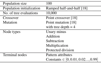
The parameters used in the experimental work are listed in Table 1.

To calculate the vicinal risk of a GP tree by Monte Carlo integration, we have used 200 samples per training datum drawn from the Gaussian kernel placed over each datum, pre-calculated and stored as an augmented training set.

Table 1 GP Parameters Used

Population size 100

Population initialization Ramped half-and-half [18] No. of tree evaluations 10,000

Crossover Point crossover [18] Mutation Point mutation [18]

with tree depth = 4 Node types Unary minus

Addition Subtraction Multiplication Protected division Terminal nodes Pattern attributes

Constants∈[0,0.01,0.02...,0.99]

3.2 Datasets

decision boundaries. For these synthetic problems, we randomly drew 100 patterns of each class to produce datasets of 200 data which were randomly partitioned into training and test partitions.

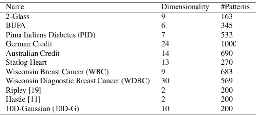
In addition to the three synthetic datasets described above, we also used eight real datasets from UCI Repository [10] to compare the performance of ERM and VRM; the validity of using the UCI datasets has been established by Soares [23]. Details of the datasets are summarized in Table 2. Most have real attributes since the formula-tion of VRM implicitly makes this assumpformula-tion although some datasets also contain categorical attributes which we have mapped to integers in the order in which they are described in the UCI documentation. 2Glass is a 2-class dataset generated from the original 6-class UCI dataset to classify float and non-float glasses. The Pima In-dians Diabetes dataset is the version due to Ripley3with the incomplete/implausible records removed.

Table 2 Details of Datasets

Name Dimensionality #Patterns

2-Glass 9 163

BUPA 6 345

Pima Indians Diabetes (PID) 7 532

German Credit 24 1000

Australian Credit 14 690

Statlog Heart 13 270

Wisconsin Breast Cancer (WBC) 9 683

Wisconsin Diagnostic Breast Cancer (WDBC) 30 569

Ripley [19] 2 200

Hastie [11] 2 200

10D-Gaussian (10D-G) 10 200

3.3 Testing Methodology

To gauge the statistical significance of the results, we have used the Wilcoxon two-sided non-parametric test [7], comparing the pairs of test error estimates resulting from each training partition for empirical and vicinal risks. Although lacking the power of parametric tests, Demˇsar [7] points-out that the necessary assumptions re-quired by parametric tests are typically violated in machine-learning situations, and so the Wilcoxon test is preferred; see [7] for further details. We have performed the Wilcoxon test by making fifteen [16] random splits of each dataset into equal-sized partitions, using one as a training set and the other as a test set.

In order to allow for the stochastic nature of GP, the estimate of test error for every split was taken as the median of 30 runs (i.e., a total of 15×30=450 runs per dataset) with an independently-generated initial population for each run. The single individual selected from each MOGP run for inclusion in the statistical analysis was the individual in the final population with either:

– The smallest training error over the whole (final) population. OR

– The smallest error over the test partition from the Pareto front.

We have included individuals with the smallest training error since these are what would be used in a single objective GP method and thus allow comparison with our MOGP approach.

Ideally, the training, validation and test procedures should all be conducted with three disjoint partitions of the dataset [11] although in practice, the the limited size of many datasets dictates a more pragmatic approach. Considering the typical procedure used in single-objective GP (SOGP), an investigator would perform multiple, often 30, GP runs each with independently-generated initial populations and report the best test error over the multiple runs. Each of this sequence of SOGP runs would return a candidate model (i.e. a hypothesis) so the process of selecting the hypothesis with the smallest error is actually amodel selectionprocedure. Our model selection procedure is thus entirely equivalent to that typically used in SOGP apart from the (immaterial) means by which the candidate hypotheses are generated: the Pareto set of candidates obtained from a single MOGP run, or thirty candidates, one obtained from each of a sequence of thirty SOGP runs. We prefer MOGP because the candidate set spans the range of model complexities from low to high, which cannot be guaranteed by independent SOGP runs.

In addition, the estimate of test error for a given individual is a single realization of a random variate so in order to mitigate the chance of this single ‘draw’ coming from the low-error extreme of the error distribution, it is desirable to make the stan-dard error of the estimate as small as possible. This has dictated our use of half of the data for the test partition since the standard error falls as a square root of the test set size.

For each dataset, we have used a single, optimized value ofσ2_{for every} smooth-ing kernel determined ussmooth-ing the procedure outlined in Section 4.1. To facilitate a single value of σ2 _{on each dimension, we normalized each attribute to unit} vari-ance over every training partition and then normalized the test partition using the same scaling. Chapelle et al. [3] assigned individually-optimized values of σ2 _to each training datum although we have adopted a simpler strategy here; potentially individually-assigned values ofσ2_{may improve the performance of VRM by} pro-ducing a locally-smoother approximation toP(x,y).

4 Results

4.1 Correlation with Test Error

and test error which displays a clear, single minimum such that minimizing the risk functional over the training set invariably leads to the lowest possible test error.

Fig. 3 Correlation between training and test errors for empirical risk. Hastie dataset; 50 training data per class.

The correlation plot for ERM with 50 training data per class in Figure 3 dis-plays vertical striations reinforcing the fact that this is a one-training-error-to-many-possible-test-errors mapping. The minimum test error does not coincide with min-imum training error and there is evidence of overfitting bymanyindividuals. Log-ically, the GP optimization could discover the optimal decision surface by chance which should return the Bayes-optimal test error but the key issue here is that this optimal solution could not be systematically identified using ERM due to its one-to-many nature.

con-(a)σ2₌₁

×10−4_{. (b)σ}2₌₁ ×10−2_.

(c)σ2_=1×10−1_{. (d)σ}2_=1.

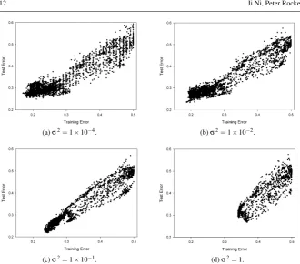
Fig. 4 Correlation between training and test errors for VRM for a range of values ofσ2_{. Hastie dataset;}

50 training data per class.

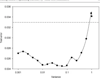
sideringσ2_{∈ {10}−3_,10−2_,10−1_,100_{}. A typical but more detailed plot of expected} test error over 15 replications againstσ2_{is shown in Figure 5 for the WDBC dataset,} for the best-performing individuals from the Pareto front. A clear although reassur-ingly broad minimum is apparent allowing an appropriate determination ofσ2_which justifies the coarse tuning ofσ2_{described above. The horizontal dashed line in} Fig-ure 5 is the corresponding expected test error for ERM. It is clear that VRM produces a significantly lower error values – we consider statistical testing of differences in errors in the next section.

Fig. 5 Expected test error over fifteen data partitions vs.σ2_{for the WDBC dataset. The dashed line is the}

best mean-of-medians test error for ERM.

of data, and iii) ERM yields a slightly smaller test error (0.2509 vs. 0.2581) although it is questionable whether this is significant. Nonetheless, the more densely-spaced training data require a smaller value ofσ2_{than 0.1 to smooth the empirical} distri-bution. (We have made no further attempt to optimize the value of σ2_{. Rather we} present the result for a sub-optimal value to reinforce the point that the value ofσ2 needs to be tuned to the training dataset at hand. The identical phenomenon is seen in Figures 4 and 5.

(a) Vicinal Risk Minimization (σ2_{=0.1) (b) Empirical Risk Minimization}

Fig. 6 Correlations between training and test errors for VRM (σ2_{=0.1), and ERM for the Hastie dataset;}

4.2 Results over Real and Synthetic Datasets

The average of the median test errors over fifteen repeated partitionings on each dataset are shown in Tables 3 and 4 in the case of VR for optimized values ofσ2 .

– Table 3 shows the results for the individuals with the lowest value of training error in the final populations – either empirical or vicinal risk.

– Table 4 shows the results for the individuals with the lowest errors over each test partition taken from the whole Pareto front.

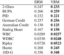
In Tables 3 and 4, the lowest errors are shown bold font. A number of observations can be made from these results.

Firstly, VRM displays the consistently lowest test errors across all datasets in both tables. From a statistical perspective, a Wilcoxon test returnsW+=66 andW−= 0, whereW+is the sum of ranks for datasets where ERM delivers a larger test error than VRM [7], andW−the converse4. We obtain ap-value of<0.01. There is thus very little evidence to support the null hypothesis that the median test errors for ERM and VRM are identical5.

Second, although minimizing some risk over a training set might be naively pre-sumed to yield the best test error, from the arguments concerning regularization and model selection set-out above, it is clear from comparing values of ERM in Tables 3 and 4, and also VRM across these two tables, that simply minimizing training risk (Table 3) does not deliver the best generalization. A model selection stage over each test partition (Table 4) selects better generalizing models. This procedure is well-established in the conventional machine learning field – see [11, pp. 222-223]. In the multiobjective optimization literature, this procedure is known aspreference ar-ticulation [5]. A statistical comparison along the same lines to that detailed in the paragraph above again yields a p-value of <0.01, yet again very little evidence to support the null hypothesis that the median errors for the two model selection meth-ods (smallest training error vs. best test partition error) are identical, implying that preference articulation is necessary for the best outcome.

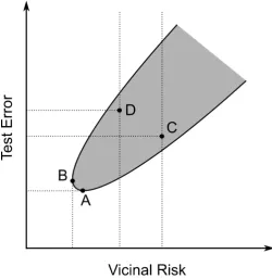
The reason for the superiority of preference articulation is illustrated by Figure 7 which depicts the region around the cusp of the plot of test error versus vicinal risk; the shaded region shows the envelope of correspondences between test error and vicinal risk which can be observed in Figure 4c. Considering first the cusp at the bottom left hand corner of the envelope region in Figure 7. Point ‘B’ is the minimum of vicinal risk whereas point ‘A’ is the minimum of test error. Thus a slightly larger vicinal risk value corresponds to the exact minimum of test error. GP is, of course, a stochastic minimizer with no guarantee of reaching an exact optimum. Therefore consider two plausible points from the Pareto front, ‘C’ and ‘D’ which are proximate to the minimum of vicinal risk (’B’) but not coincident with it – i.e., ‘C’ and ‘D’ are approximate minima of VR. It is clear for this possible outcome that point ‘C’ will

4 _{The sum of ranks 1 to 11 = 66.}

5 _{In this paper we make what may seem to be rather cautious statements about the outcome of hypothesis}

deliver a lower value of test error than ‘D’ despite having a higher value of vicinal risk. This explains why a separate model selection stage can deliver a smaller value of test error than just minimizing vicinal risk. Notwithstanding this, vicinal risk has a more desirable characteristic than empirical risk – see Figure 3. Further, we show below that VRM produces statistically improved values of test error compared to ERM, as well as having greater repeatability and other properties.

Fig. 7 Illustration of the region around the cusp of the test error/vicinal risk correlation plot showing the justification for a preference articulation stage.

Third, although not shown in Tables 3 and 4, the variancesof the median test errors averaged over all partitions are quite similar for ERM and VRM for a given dataset, and larger than would be suggested by the variances over any single partition. The explanation is simply that the variance of these values is dominated by the vari-ability due to sampling the multiple training partitions rather than the variablility due to the classifiers. For this reason, the variances of the aggregated test partition errors in Tables 3 and 4 cannot be used for gauging statistical significance although lower averaged median values are still meaningful. We present paired tests below which eliminate this extraneous variability below.

improvements in performance as this limit is approached are likely to be increas-ingly difficult to achieve. VRM’s improvement on already-good performance is thus noteworthy.)

Table 3 Averaged median test errors for individuals with the best training error; smallest values are shown in bold face.

ERM VRM

2-Glass 0.290 0.284

BUPA 0.300 0.292

PID 0.248 0.236

German Credit 0.272 0.268

Australian Credit 0.143 0.134

Statlog Heart 0.194 0.165

WBC 0.0339 0.0311

WDBC 0.0391 0.0317

Ripley 0.0877 0.0607

Hastie 0.302 0.286

10D-G 0.417 0.391

Table 4 Averaged median test errors for the best individuals on the Pareto front; smallest values are shown in bold face.

ERM VRM

2-Glass 0.247 0.233

BUPA 0.266 0.259

PID 0.232 0.221

German Credit 0.257 0.256

Australian Credit 0.130 0.125

Statlog Heart 0.167 0.150

WBC 0.0289 0.0257

WDBC 0.0330 0.0248

Ripley 0.0720 0.0523

Hastie 0.268 0.245

10D-G 0.356 0.348

Within each dataset, we can compare VR (for optimizedσ2_{) with empirical risk} using the Wilcoxon test. Results over the fifteen data partitions are summarized in Table 5 (selected individuals with the lowest training error), and Table 6 (selected individuals with lowest test partition error).W+ is the sum of ranks for partitions for which ERM produces larger test error than VRM, andW−the converse. As be-fore, we have taken the median test error over 30 independently-initialized runs as representative of the test error over each of the fifteen partitions.

gener-Table 5 Wilcoxon’s test comparing 0/1 loss and VRM within each dataset; selected individuals with the lowest training set error

Dataset Optimalσ2 _{W-score p-value}

2D-Glass 10−2 _W+_=61.5W−_{=29.5 =0.26}

BUPA 10−3 _W+_=92.5,W−_{=12.5 <0.02}

PID 100 W+=91.5,W−=13.5 <0.02 German 10−1 _W+_=105.5,W−_{=14.5 <0.01}

Australian 100 _W+_=105,W−_{=0 <0.01}

Statlog Heart 100 _W+_=91.5,W−_{=13.5 <0.02}

WBC 10−1 _W+_=42,W−_{=3 ≤0.02}

WDBC 10−1 W+=120,W−=0 <0.01 Ripley 10−1 _W+_=75,W−_{=3 <0.01}

Hastie 10−1 _W+_=84.5,W−_{=20.5 <0.05}

10D-G 100 _W+_=97.5,W−_{=7.5 <0.01}

Table 6 Wilcoxon’s test comparing 0/1 loss and VRM within each dataset; selected individuals with the lowest test partition error on the Pareto front.

Dataset Optimalσ2 _{W-score p-value}

2D-Glass 10−2 W+=91,W−=0 <0.01 BUPA 10−3 _W+_=105,W−_{=0 <0.01}

PID 10−1 W+=91,W−=0 <0.01 German 10−1 _W+_=52,W−_{=26 =0.30}

Australian 100 _W+_=91,W−_{=0 <0.01}

Statlog Heart 100 W+=105,W−=0 <0.01 WBC 10−1 _W+_=69,W−_{=9 ≤0.02}

WDBC 10−1 W+=120,W−=0 <0.01 Ripley 10−1 _W+_=76,W−_{=2 <0.01}

Hastie 10−3 _W+_=91,W−_{=0 <0.01}

10D-G 10−1 W+=66,W−=12 <0.05

ally delivers superior results and, at very worst, two results which are not statistically different. In no case is ERM superior to VRM. (It should also be noted that 2D-Glass VRM vs. ERM produced 8 ‘wins’ for VRM and 5 ‘losses’ out of 15 pairwise com-parisons; for the German Credit dataset, the corresponding figures are 8 ‘wins’ and 4 ‘losses’. That is, VRM still performs better on raw count.)

From Tables 5 and 6, it is obvious that the optimal value ofσ2_{and the apparent} superiority of VRM both vary by dataset which is expected as each problem has different characteristics.

4.3 Stability of Training

his-togram. We present two histograms of test error for the real WDBC dataset, for two randomly selected data partitions in Figure 8, and two corresponding histograms for the synthetic Ripley dataset in Figure 9.

It can be seen from Figures 8 and 9 that the histograms for VRM are more com-pact with modes at lower values of test error than for ERM, indicating that VRM training is, on average, more stable and more likely to deliver a lower test error.

5 Discussion

In essence, what we are doing in the VRM approach is to form a ‘better’ approxima-tion of the underlying class-condiapproxima-tioned densities by smoothing-out the set of discrete samples in the training set. In this sense,σ2_{is another kind of regularizing} param-eter which needs to be adjusted to obtain best results. Similar although differently-motivated approaches have previously been employed with multi-layer perceptron (MLP) neural networks. For example, Holmstr¨om and Koistenen [12] obtained im-proved generalization performance by adding Gaussian-distributed noise to the train-ing set in an ad hoc manner. Karystinos and Pados [14] employed a much more elab-orate approach of modeling the distribution of input variables and then drawing a large, similarly-distributed training set which yielded improved performance.

Placing Gaussian kernels over a training data is Parzen window density estima-tion [8] where the width of the kernels is a smoothing parameter which has to be tuned, typically by cross-validation. Under Parzen window estimation, the probability density function (PDF) of each class is approximated by a (normalized) summation of Gaussian kernels. Assuming a two-class problem (‘A’ vs. ‘B’) and the approximation of the class-conditioned PDF for class ‘A’ is given by ˜pA(x|A), the risk associated

with misclassifying a pattern drawn from ‘A’ is given by:

R_A=

Z

Ω ˜

pA(x|A)dx (8)

wherex_∈RN_{and the region of integration,}Ω_{is the portion ofN-dimensional pattern}

space to the right of the decision surface in Figure 10. A similar argument holds for class ‘B’ which can be approximated by ˜pB(x|B)and where the integral definingRB

is taken over the region of space in Figure 10 to theleftof the decision boundary, namely the complement ofΩ_{. The overall probability of error,P(error)is given by}

a weighted sum ofR_AandR_B:

P(error) =κ_ABP(A)R_A+κ_BAP(B)R_{B (9)}

whereκ_{i j is the cost of misclassifying a pattern from classi as belonging to class}

j which we can, without loss of generality, assume to be unity.P(A)andP(B)are the prior probabilities of classes ‘A’ and ‘B’, respectively. By selection of an ap-propriate decision surface (i.e., by classifier training), (9) can be minimized to yield (close to) the Bayes’ optimal error. Since ˜pk(x|k),k∈ {A,B}are approximated by a

(a) Partition #1

(b) Partition #8

(a) Partition #3

(b) Partition #11

Fig. 10 Illustration of the domain of integration over pattern space to calculate risks.

such thatg(x)−t >0 and the majority of the points in the other class such that g(x)−t<0. VRM can thus be directly related to minimizing the overall probability of error. The significant advantage of the formulation presented in this paper is that the class-conditioned risks R_{A,B (8) are evaluated in the 1D decision space rather}

than inN-dimensional pattern space over, typically, a region of integration defined by a highly non-linear decision surface. (Indeed, in our experience, GP classifiers can frequently generate disjoint decision regions in pattern space.)

As to why vicinal risk does not exhibitperfect correlation with test error (Sec-tion 4.1), obviously the (implicitly) assumed forms for ˜pA,B(x|A,B)are

approxima-tions and therefore incur some error. Nonetheless, VRM is able to consistently guide the optimization to consistently superior regions of the solution space and is thus a demonstrable improvement over ERM.

Finally, implementation of VRM training used here is very simple and amounts to drawing an augmented training set, in advance, from the Parzen density estimate of the original data. For the case of small datasets where the ill-posedness due to the 0/1 loss is most problematic, the use of Monte Carlo integration is not a significant burden although we can envisage an ‘early jump-out’ technique to speed-up the com-putations. The integral for thei-th pattern is evaluated by counting the fraction of the augmented samples from this pattern that falls on the wrong side of the decision surface – see Figure 2. Only training patterns proximate to the decision surface are likely to be misclassified – patterns a long way from the decision boundary will never be misclassified. Therefore, if the firstnMonte Carlo samples from thei-th pattern are all correctly classified, there is a probably little value in considering the remain-ing samples; to some confidence level, we can thus ‘jump-out’ the integral evaluation early for thei-th pattern since it is likely to contribute nothing to the vicinal risk. This is an area for future investigation.

6 Conclusions

In this paper we have introduced and motivated vicinal risk minimization (VRM) for training genetic programming classifiers. VRM is formulated by placing a Gaussian kernel on each training datum in pattern space and propagating the resulting errors on the decision into the 1D decision space. Minimizing vicinal risk over the training set is shown to be equivalent to approximately minimizing the overall probability of error for the problem in a Bayesian setting. VRM is shown to be far better correlated with test error than empirical risk minimization (ERM), that is, minimizing vicinal risk leads to consistently improved classifier generalization. The widths of the Gaussian kernels can be straightforwardly chosen by cross-validation.

We present statistical comparisons between ERM and VRM which indicate there is very little evidence to support the null hypotheses that the two loss functions per-form identically. VRM is shown not to completely remove the need for a model selection stage over the Pareto front of equivalent solutions although there is good evidence that it guides the evolutionary optimization to improved solutions.

Acknowledgements The authors would like to thank Yilong Cao and Richard Everson for valuable dis-cussions.

References

1. Amil, N.M., Bredeche, N., Gagn´e, C., Gelly, S., Schoenauer, M., Teytaud, O.: A statistical learning perspective of genetic programming. In: 12th_{European Conference on Genetic Programming} (Eu-roGP 2009), pp. 327–338. T¨ubingen, Germany (2009)

2. Borges, C.E., Alonso, C.L., Monta˜na, J.L.: Model selection in genetic programming. In: 12th_Annual Conference on Genetic and Evolutionary Computation (GECCO 2010), pp. 985–986. Portland, OR (2010)

3. Chapelle, O., Weston, J., Bottou, L., Vapnik, V.: Vicinal risk minimization. In: Advances in Neural Information Processing Systems 13 (NIPS 2000), pp. 416–422. Denver, CO (2000)

5. Coello, C.A.C., Lamont, G.B.: Applications of Multi-Objective Evolutionary Algorithms, vol. 1. World Scientific, Singapore (2004)

6. Cohen, J.: The earth is round (p< .05). Am. Psychol.49(12), 997–1003 (1994)

7. Demˇsar, J.: Statistical comparisons of classifiers over multiple data sets. J. Mach. Learn. Res.7, 1–30 (2006)

8. Duda, R.O., Hart, P.E., Stork, D.G.: Pattern Recognition, 2nd edn. John Wiley & Sons, New York (2001)

9. Ek´art, A., N´emeth, S.Z.: Selection based on the Pareto nondomination criterion for controlling code growth in genetic programming. Genet. Program. Evol. M.2(1), 61–73 (2001)

10. Frank, A., Asuncion, A.: UCI Machine Learning Repository. University of California, Irvine, School of Information and Computer Sciences (2010). URLhttp://archive.ics.uci.edu/ml 11. Hastie, T., Tibshirani, R., Friedman, J.: The Elements of Statistical Learning: Data Mining, Inference,

and Prediction, 2nd_{edn. Springer-Verlag (2009)}

12. Holmstr¨om, L., Koistinen, P.: Using additive noise in back-propagation training. IEEE T. Neural. Networ.3(1), 24–38 (1992)

13. Iba, H., de Garis., H., Sato, T.: Genetic programming using a minimum description length principle. In: Advances in Genetic Programming, pp. 265–284. MIT Press (1994)

14. Karystinos, G.N., Pados, D.A.: On overfitting, generalization, and randomly expanded training sets. IEEE T. Neural. Networ.11(5), 1050–1057 (2000)

15. Kumar, R., Rockett, P.I.: Improved sampling of the Pareto-front in multiobjective genetic optimiza-tions by steady-state evolution: A Pareto converging genetic algorithm. Evol. Comput.10(3), 283–314 (2002)

16. Nadeau, C., Bengio, Y.: Inference for the generalization error. Mach. Learn.52(3), 239–281 (2003) 17. Polak, E.: Optimization: Algorithms and Consistent Approximations. Springer, New York (1997) 18. Poli, R., Langdon, W.B., McPhee, N.F.: A Field Guide to Genetic Programming. Published viahttp:

//lulu.comand freely available athttp://www.gp-field-guide.org.uk(2008)

19. Ripley, B.D.: Neural networks and related methods for classification. J. Roy. Stat. Soc. B Met.56(3), 409–456 (1994)

20. Rissanen, J.: Modeling by shortest data description. Automatica14(5), 465–471 (1978)

21. Robert, C.P., Casella, G.: Monte Carlo Statistical Methods, 2nd edn. Springer-Verlag, New York (2005)

22. Silva, S., Dignum, S., Vanneschi, L.: Operator equalisation for bloat free genetic programming and a survey of bloat control methods. Genet. Program. Evol. M.13(2), 197–238 (2012)

23. Soares, C.: Is the UCI repository useful for data mining? In: 11th_{Portuguese Conference on Artificial} Intelligence (EPIA 2003), pp. 209–223. Beja, Portugal (2003)

24. Tikhonov, A.N., Arsenin, V.Y.: Solutions of Ill Posed Problems. V.H. Winston, Washington, D.C (1977)

25. Vapnik, V.N.: The Nature of Statistical Learning Theory, 2nd_{edn. Springer, New York (2000)} 26. Zhang, Y., Rockett, P.: A comparison of three evolutionary strategies for multiobjective genetic

pro-gramming. Artif. Intell. Rev.27(2-3), 149–163 (2007)