This is a repository copy of The composition of wage differentials between migrants and natives.
White Rose Research Online URL for this paper: http://eprints.whiterose.ac.uk/82782/
Version: Accepted Version
Article:
Nanos, P. and Schluter, C. (2014) The composition of wage differentials between migrants and natives. European Economic Review, 65. pp. 23-44. ISSN 0014-2921
https://doi.org/10.1016/j.euroecorev.2013.10.003
Article available under the terms of the CC-BY-NC-ND licence (https://creativecommons.org/licenses/by-nc-nd/4.0/)
Reuse
Unless indicated otherwise, fulltext items are protected by copyright with all rights reserved. The copyright exception in section 29 of the Copyright, Designs and Patents Act 1988 allows the making of a single copy solely for the purpose of non-commercial research or private study within the limits of fair dealing. The publisher or other rights-holder may allow further reproduction and re-use of this version - refer to the White Rose Research Online record for this item. Where records identify the publisher as the copyright holder, users can verify any specific terms of use on the publisher’s website.
Takedown
If you consider content in White Rose Research Online to be in breach of UK law, please notify us by
The Composition of Wage Differentials between Migrants and
Natives
Panagiotis Nanosa, Christian Schluterb,a
a
Economics Division, University of Southampton, Highfield, Southampton, SO17 1BJ, UK b
Aix-Marseille Universit´e (Aix-Marseille School of Economics) , CNRS & EHESS, Centre de la Vieille Charit´e, 13002 Marseille, France
September 2013
Abstract
We consider the role of unobservables, such as differences in search frictions, reservation wages, and productivities for the explanation of wage differentials be-tween migrants and natives. We disentangle these by estimating an empirical general equilibrium search model with on-the-job search due to Bontemps et al. (1999) on segments of the labour market defined by occupation, age, and nationality using a large scale German administrative dataset.
The native-migrant wage differential is then decomposed into several parts, and we focus especially on the component that we label “migrant effect”, being the difference in wage offers between natives and migrants in the same occupation-age segment in firms of the same productivity. Counterfactual decompositions of wage differentials allow us to identify and quantify their drivers, thus explaining within a common framework what is often labelled the unexplained wage gap.
Keywords: immigrants, decomposition of wage differentials, job search, turnover
JEL Classification: J31, J61, J63
1. Introduction
The empirical literature on the labour market experience of immigrants often focuses on differences in observable characteristics between migrants and natives to explain wage differentials. Less explored is the role of unobservables, such as differ-ences in search frictions, reservation wages, and productivities. Yet, it is precisely
Email addresses: [email protected](Panagiotis Nanos), [email protected](Christian Schluter)
these factors that modern search theory emphasises to be important for wage dis-persion. We examine and disentangle the role of these various unobservables in explaining migrant-native wage differentials by adapting to the migrant context the empirical general equilibrium search model with on-the-job search due to Bontemps et al. (1999).
The estimation of this structural model on segments of the labour market defined by occupation, age, and nationality enables us to decompose the native-migrant wage differential into several parts. In particular, we focus on the component that we la-bel “migrant effect”, being the difference in wage offers between similar native and immigrant workers in firms of the same productivity. This effect is of interest as we thus control for firm-level differences as measured by their productivities, which have recently been shown using firm-level data to contribute systematically to the wage gap (Aydemir and Skuterud (2008) in the case of Canada, de Matos (2012) for Portu-gal, and Bartolucci (2013b) for the German case).1 One particular advantage of our approach is that we do not require firm-level data (data confidentiality promises usu-ally deny public access), as the productivity distribution emerges as an equilibrium relationship. We estimate the migrant effect on internationally accessible German administrative data, the scientific use file known as IABS which is a 2% subsample of the German employment register. This enables us to contribute to the recent lit-erature on the immigrant-native wage gap as follows. While the role of observables is well understood for explaining the wage gap, the role of unobservables is less so. Such wage gaps arise when, for instance, migrants have systematically lower reservation wages (whose role is examined in detail in Albrecht and Axell (1984)), or when firms in a migrant-native segmented labour market (which we discuss below) are less pro-ductive in the migrant segment, or when wage-posting firms in one segment derive greater monopsony power from e.g. greater search frictions. Our analysis focuses on the roles of differences in the job turnover parameters, behavioural differences induced by differences in reservation wages, and productivity differences.2 Within
1
The migrant effect corresponds to within-firm wage differentials of workers with similar observ-able characteristics reported in these papers.
2
a common framework, we establish the relative importance of each of these factors. Having estimated the model’s parameters and thus the actual wage gap and migrant effect, we quantify the roles of the various unobservables in several counterfactual experiments.
The structural model is estimated on a large German administrative panel. Ger-many is a particularly interesting and relevant case since it hosts the largest numbers of foreign nationals in Europe, and immigration is known to be predominantly low-skilled. According to Eurostat, 7.13 million foreign nationals resided in Germany in 2010, about 8.7% of the total population. The size of the IABS allows us to strat-ify the analysis by nationality, occupation and age. The resulting subsamples are sufficiently large to permit precise estimation of the model’s structural parameters. Moreover, since this is administrative data, the usual concerns about the quality of survey data in a migrant context (sample size, measurement accuracy, and use of retrospective information) are absent.
We briefly describe some aspects of our applications of the structural model. In or-der to control for heterogeneity in observables, we follow common estimation practice in the search-theory literature by partitioning the labour market into many segments. These segments are defined in terms of occupation, age, and nationality.3 Given the skill profile of migrants, we consider only the low and medium skill occupations. Each segment is thus assumed to be potentially a separate labour market, characterised by its own job turnover parameters (the job arrival and separation rates). Turning to the unobservables (for the econometrician), firms in each segment differ in terms of productivity, and workers differ in terms of reservation wages. Such reservation wage heterogeneity is plausible given the absence of a legal minimum wage in Germany, and the fact that the location decisions of labour migrants in Roy-style models are usually based on comparisons of expected incomes in source and host country. Mi-grants might trade-off wage and non-wage job characteristics differently to natives, given their well-known clustering. Besides this preference component, reservation wages also feature an institutional one, but this is less important as contributory unemployment insurance benefits are independent of immigrant status.
The assumption of separate markets for natives and immigrants and the
associ-Hirsch et al. (2010) consider the gender wage gap in the light of this. We relate the migrant effect to the Hirsch and Jahn (2012) analysis of monopsonistic discrimination in Section 2.4.
3
The term “nationality” rather than “immigrant status” is used here for greater precision given the coding practices of the German Statistical Office. Most German data sources record nationality and not country of birth since German nationality was conferred by descent until the year 2000,
ated notion of job segmentation conforms to existing international empirical evidence. For instance, using Portuguese data, de Matos (2012) shows that immigrants “work in different industries and occupations than natives” (p.10), and the sorting of im-migrants is also observed by Aydemir and Skuterud (2008) for Canada. As regards Germany, D’Amuri et al. (2010) observe that recent immigrants are significantly more likely to compete with established immigrants rather than with natives. Vel-ling (1995) is an early paper to report “evidence of strong occupational segregation” (p.1) between natives and immigrants. This finding has recently been reaffirmed by Lehmer and Ludsteck (2011), Br¨ucker and Jahn (2011), Bartolucci (2013b), and Glitz (2012) who concludes that “ethnic segregation [..] is endemic in the German labour market” (p.15).4 This segmentation is also consistent with the evidence of strong occupational immobility we find in our data (which has also been observed for other countries, e.g. by de Matos (2012) for Portugal).5
For each occupation-age segment, we estimate using maximum likelihood the job turnover parameters, the parameters characterising the reservation wage distribution, and the firms’ productivity distribution. We find substantial differences in Germany between natives and foreigners. The segment-specific raw average log wage gaps in our data range from .09 to .45, the overall log wage gap being .22, which is in line with reports in the literature for Germany (e.g. Dustmann et al. (2010) report an unconditional average log wage gap of .23, Hirsch and Jahn (2012) report a gap of .2, while Lehmer and Ludsteck (2011) report predicted wage gaps ranging from .08 to .44 depending on nationality). Turning to the qualitative implications of our model estimates, we find that migrants experience job separations more often than natives but also find jobs more quickly. However, the net effect is such that migrants typically experience greater search frictions. The job turnover parameters decline in age. Across all segments and nationality, transitions into new jobs happen more
4
At the same time, these papers provide complementary perspectives on the native-immigrant wage gap in Germany: descriptive Oaxaca-Blinder decompositions (Velling (1995), Lehmer and
Ludsteck (2011)), wage setting (Br¨ucker and Jahn (2011)), monopsonistic discrimination (Hirsch
and Jahn (2012)), while Bartolucci (2013b) provides an interpretation in terms of taste-based discrimination. D’Amuri et al. (2010) pursue a different concern and estimate the wage and em-ployment effects of recent immigration in Western Germany (and find little evidence for adverse effects on native wages and employment levels).
5
quickly than transitions into unemployment. This finding of migrants’ higher job separation and offer rates is consistent with differences in employment protection; in particular, Sa (2011) reports that migrants in Germany are much more likely than natives to work on temporary contracts. As regards the reservation wage distribution, there are some workers in all segments with high reservation wages who turn down new job offers when wage offers are too low. However, migrant workers are less demanding on average than natives.
Migrants receive wage offers that are lower than those for natives controlling for the same productivity. This migrant effect is the largest for clerks and service work-ers, and small for unskilled workers. In particular, the average migrant effect for the skilled ranges between 12% and 15% of the average wage gap, and for clerks and service workers the range is 23% to 39%. For all occupation groups, the migrant effect declines across age groups. These estimates imply that the largest part of the within-group native-migrant wage gap is explained by differences in the produc-tivity distribution (one explanation for such producproduc-tivity differences is advanced in de Matos (2012)). At the same time, the migrant effect is significant in many seg-ments, and, if expressed in terms of the average segment-specific wage of natives, it is found to be consistent with estimates of “unexplained wage differences” reported in the literature for Germany based on standard Oaxaca-Blinder decompositions (for instance, Lehmer and Ludsteck (2011) report a range from 4 to 17%) or comple-mentary approaches (Hirsch and Jahn (2012) report 6% while Bartolucci (2013b) suggests discrimination effects ranging between 7 and 17%). Our counterfactual de-composition approach allows us to quantify the (marginal and joint) roles of the underlying drivers of the migrant effect in terms of labour market turnover param-eters and behavioural differences captured by the reservation wage distribution. We find that reducing the job separation rate for migrants to that of natives typically leads to a large reduction in the migrant effect. This is of interest to policy makers since this parameter is targetable by e.g. deploying measures to improve migrants’ employment protection.
2. The Analytical Framework
The search model with wage-posting and on-the-job search has been described and discussed extensively before in the literature. Therefore, only its most salient features will be outlined. We use the extension of the Burdett and Mortensen (1998) model, and the subsequent empirical generalisation and implementation of van den Berg and Ridder (1998), due to Bontemps et al. (1999). This extends the basic set-ting by introducing productivity heterogeneity among firms, which improves the fit of the model to wage data, and heterogeneity among workers in terms of the unob-served opportunity cost of employment, which improves the fit to the unemployment duration data. As discussed above, the latter is very plausible in the migration context against the background of Germany’s institutional rules.
The labour market is partitioned into many segments, defined in our empirical implementation by age, occupation and nationality. Each segment is considered as a labour market for which the following model and estimation approach applies. The structural parameters are of course allowed to vary across segments, but for notational simplicity we suppress a segment index. This segmentation assumption precludes individuals moving from one segment to another, which is consistent with the evidence of occupational immobility in Germany presented below and the exter-nal evidence discussed in the Introduction. If the labour market is integrated over some stipulated segments, then the estimates of the structural parameters should be the same statistically; the segments can then be added to improve estimation effi-ciency. In line with the segmentation hypothesis we find that the estimated structural parameters differ across occupation-age-nationality groups. We proceed to outline the model for one labour market segment.
2.1. The Model of a Labour Market Segment
The labour market segment is populated by a fixed continuum of workers with measureM, and a fixed continuum of firms with measure normalised to one. Firms differ in terms of (the marginal) productivity (of labour) pwith distribution Γ. Un-employed workers differ in terms of their reservation wages b with distribution H.
At any point in time, a worker is either unemployed or employed, and searches for jobs both off and on the job. Individuals draw offers by sampling firms using a uniform sampling scheme. Jobs are terminated at the exogenous rateδ, and job offers arrive at the common rate λ irrespective of the worker’s state. This is a restrictive assumption but necessary for identification.6 Let k=λ/δ.
6
Job offers are, of course, unobservable to the econometrician. The job offer distri-bution is denoted byF, whereas the observable wage or earnings distribution (i.e. of accepted wages) is denoted by G. Let [w, w] denote the support of F, and, for nota-tional convenience, F = [1−F]. F is related toG through an equilibrium condition implied by the theoretical structure. Firms post wages and there is no bargaining.7
Workers are risk neutral and maximise their expected steady state discounted fu-ture income. Their optimal strategy has the reservation wage property: an employed individual moves to a new employer if the offered wage exceeds the current wage (so the model does not allow for wage cuts); an unemployed individual accepts a new job if the offer exceeds b, and otherwise rejects the offer and remains unemployed. On-the-job search thus generates further ex-post heterogeneity in reservation wages. In steady-state equilibrium, the flows of workers into and out of the unemploy-ment pool are equal, which determines the unemployunemploy-ment rateu. Consider the stock of employed workers who earn a wage less than or equal tow. Two sources constitute the outflow from this stock, namely: (i) exogenous job separations at rateδ and sub-sequent transits into unemployment, and (ii) wage upgrading as employed workers move to poaching firms. The combined outflow is thus (1−u)G(w)(δ +λF(w)). The flow into this stock consists of unemployed individuals who receive wage of-fers above their reservation wage. Conditional on b, the probability of this event is
uλ[F(w)−F(b)]. The marginal inflow is obtained by integrating up to w over the distribution of b in the stock of the unemployed. Denoting the latter by Hu, the
steady state equation for the labour market yields the relationship betweenHu and H, namelyuHu(b) =
Rb
−∞[1 +kF(x)]
−1dH(x).
Equating inflows and outflows relates the wage offer distributionF to the realised wage distributionG. To be precise, Bontemps et al. (1999, Proposition 2) show that the unemployment rate uand the actual wage distribution Gsatisfy
u=
1
1 +kH(w) +
Z w
w
1
1 +kF (x)dH(x)
+ [1−H(w)] (1)
employment: it is simply equal tob. If job offer arrival rates were to differ, Mortensen and Neumann
(1988) show that this opportunity cost would be an intractable function of all the primitives of the model, leading to feedback to workers’ optimal strategies from wages and firm behaviour.
7
G(w) = H(w)−
1 +kF (w)h 1
1+kH(w) +
Rw
w
1
1+kF(x)dH(x)
i
1 +kF (w)
(1−u) . (2)
Risk neutral firms have constant-returns-to-scale technologies, and post wages that maximise steady state profit flows, the profit per worker beingp−w. Firms do not observe the reservation wage of a potential employee. In equilibrium, firms offer wages to workers that are smaller than their productivity level, so firms have some monopsony power. Bontemps et al. (1999, Proposition 9) show that in equilibrium there exists an increasing function K which maps the productivity distribution Γ into the wage offer distributionF, so that the wage offer satisfies w=K(p) with
K(p) = p−
"
p−w
(1 +k)2H(w) +
Z p
p
H(K(x))
1 +k[1−Γ (x)]2dx
#
[1 +k[1−Γ (p)]]2
H(K(p)) (3)
and F (w) = Γ (K−1(w)). Hence given the frictional parameter k, the reservation wage distributionHand the productivity distribution Γ, equation (3) yields the wage offer distribution F, which then via (1) yields the equilibrium unemployment rate and through (2) the actual wage distributionG.
Our dataset does not include measures of firm productivity but, of course, exten-sive wage data. Using expressions of the key quantities in terms of the actual wage density g, the productivity distribution Γ becomes estimable. In particular, it can be shown that
(1−u) = k
(1 +k)Rw
w g(t)
H(t)dt
, (4)
1
1 +kF(w) = (1−u) Z w
w
g(t)
H(t)dt+
1
[1 +k]. (5)
Equation (4) follows from (5) withw=w. The equilibrium productivity levels are
p=K−1(w) = w+ H(w)
2 (1−u)g(w)
1 +kF(w)
+h(w). (6)
2.2. Identification
offers. These data are sufficient to identify8 the structural parameters, once the reservation wage distribution is parametrised. We assume that H is a normal dis-tribution with unknown location and scale parameters, (µ, σ)≡θ. Since arrivals of job offers and separations are assumed to follow Poisson processes, sojourn times are exponentially distributed.
In particular, the wage data identify the wage distribution G, and the minimum and the maximum of the observed wages identify the infimumw and the supremum
w of the wage offer distribution. The steady state flow equations in form of (4) and (5) then identify the wage offer distribution F given λ/δ and H(.;θ), which yield the productivity distribution Γ via (3). The job separation rate is identified from job durations ending in a transition to unemployment, as these are exponential variates with parameter δ, the mean duration being δ−1. Job durations ending in a transition to another job with wage w are exponential with parameter λF¯(w). Together with unemployment durations ending in a transition to a job with wage
w these identify the remaining parameters λ and θ. Since the reservation wage is unobservable, the marginal unemployment durations are mixtures of exponentials, Pr{Tu ≤t|b ≤w}= 1−
Rw
−∞exp(−λF¯(b)t)dHu(b;θ|b ≤w).
Absent such mixing, when H is degenerate and all agents accept all wage offers above the common reservation wage, transitions to a new job from each labour market state would permit separate identification of the job offer arrival rates, and thus would give rise to testable overidentification restrictions. In the presence of unobservable heterogeneity captured by H, overidentification restrictions only arise with additional data that would permit, for instance, an independent estimation of the wage offer distribution (see e.g. Christensen et al. (2005) for such an approach).
2.3. Maximum Likelihood Contributions for Labour Market Segments
The preceding constructive identification argument suggests that we can estimate the structural parameters using maximum likelihood on our data on unemployment and employment durations and wages. The likelihood contributions we consider in detail next differ slightly from those in Bontemps et al. (1999) since our data are flow and not stock samples. The validation exercise reported in Appendix B verifies the good performance of our estimation procedure on artificial data. The density of accepted wages, and thus G, is estimated using kernel methods, and enters all likelihoods as a nuisance parameter.
8
Consider first the likelihood contributions of unemployed agents. Since the unem-ployment rate is a function of the model parameters, it needs to enter the sampling plan. In equilibrium, the probability of encountering an unemployed individual is given by (4). Since the reservation wage b is unobservable, it needs to be integrated out. We distinguish between individuals for whomb ≤was they accept all job offers, a mass ofH(w), and those for whomb > w as they reject offers belowb. Recall that
F(w) = 0, and we assume that all individuals included in our sample would accept at least one wage offer w∈[w, w]. This implies that the sup of H is lower than the sup ofF,b ≤w, so this specification does not take into account cases of permanently unemployed individuals. Conditional on b, the distribution of unemployment dura-tions in our flow sample is exponential with parameter λF(b). The accepted wage,
w, is a realisation of the wage offer distribution truncated at b: f(w)/F (b). The likelihood contribution of an unemployedLu is thus, having substituted out u,
Lu(λ, δ, θ) =λ(1−dr)exp (−λt)
H(w)
1 +k [f(w)]
(1−dr)
+ + Z w w (
λF(b)(1−dr)
exp[−λF(b)t]
f(w)
F (b)
(1−dr)
1
1 +kF(b) )
dH(b), (7)
where dr is a dummy variable equal to one if the spell is right-censored (the only
relevant censoring in our data). In this case it is only known that the unemployment duration exceeds t.
We turn to the likelihood contributions of employed workers, denoted byLe. The
probability of sampling an employed individual receiving a wage w is (1−u)g(w). We have further data on the job duration and the exit state. Letv be a dummy vari-able equal to one if the destination of an employment spell is unemployment, and zero if the destination is another job. We have two competing risks: Exits to unemploy-ment occur with probability δ/
δ+λF(w)
and exits to higher paying jobs occur with probability λF(w)/
δ+λF(w)
. Conditional on being employed with wage
w, the job duration has an exponential distribution with parameter
δ+λF(w)
. If a transit to unemployment is observed at duration t, this implies that the duration of the other latent risk factor exceeds t, the joint density factorises, and we have
δexp(−δt) exp(−λF(w)). Therefore
Le(λ, δ, θ) = (1−u)g(w) exp
−
δ+λF(w)
t ×nδv
λF(w)(1−v)o(1−dr)
, (8)
indicated bydr, we only know that the job duration exceeds t.
2.4. Migrants, Natives, Wage Differentials and the Migrant Effect: Concepts and Simulated Data
We develop an illustrative example in order to introduce our key concepts. Con-sider two labour market segments, one occupied by natives (N) and the other by immigrants (F). Workers in either segment exhibit the same observable characteris-tics (in our empirical application below we consider the same skill and age group). We calibrate the two segments (in line with the empirical results) as follows: the job turnover parameters of migrants are assumed to be higher than those of natives,
δF = .016 > .005 = δN and λF = .13 > .07 = λN, while natives have higher mean
reservation wages, µF = 45 < 60 = µN. The productivity distribution in the
seg-ment for natives is assumed to first order stochastically dominates that of migrants: ΓF(p) = 1−(pF/p)α and ΓN(p) = 1−(pN/p)α with α = 2.1,pF = 40, andpN = 50.
[image:12.612.161.443.352.558.2]The validation exercise reported in Appendix B discusses the estimation results.
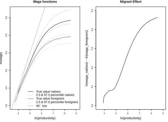
Figure 1: Wage offer curves for natives and migrants, and the “migrant effect”.
4 5 6 7 8 9
3.5
4.0
4.5
5.0
5.5
6.0
Wage functions
ln(productivity)
ln(w
age)
True value natives 2.5 & 97.5 percentile natives True value foreigners 2.5 & 97.5 percentile foreigners 45° line
4 5 6 7 8 9
0.0
0.1
0.2
0.3
0.4
0.5
Migrant Effect
ln(productivity)
ln(w
age_nativ
es) − ln(w
age_f
oreigners)
difference in wage offers between similar native and immigrant workers in firms of the same productivity: wN(p)−wF(p). This effect is of interest since we thus control
for firm-level differences as measured by their productivities.
This concept of the migrant effect suggests to decompose the aggregate wage differential9 between migrants and natives, R
AwN(p)dΓN(p)−
R
AwF(p)dΓF(p), into
the aggregate migrant effect and a weighted difference between firm productivities (whereA denotes the intersection of the supports of the productivity distributions). Solving for the aggregate migrant effect, we thus have
Z
A
[wN(p)−wF(p)]dΓN(p) =
Z
A
wN(p)dΓN(p)−
Z
A
wF(p)dΓF(p) (9)
−
Z
A
wF(p)d[ΓN(p)−ΓF(p)].
We briefly comment on the relationship between the migrant effect and the con-cept of monopsonistic discrimination, as examined in e.g. Hirsch and Jahn (2012). The latter is measured by these authors indirectly from a search-model inspired de-composition of the long run wage elasticity of labour supply using reduced-form job separation models that are estimated separately on data for migrants and natives. In our model, greater monopsony power of firms (measured by the absolute or relative distance between productivity, i.e. the 45 degree line, and wages as illustrated in Figure 1.A) in the migrant segment gives rise to the migrant effect. Our approach enables us to go beyond measuring the migrant effect, as we explain it within a com-mon framework in terms of the relative importance of differences in the job turnover parameters and behavioural differences induced by differences in reservation wages. In particular, a closer inspection of (3) shows that the wage offers are complicated functions of these structural parameters,wi(p|pi, αi, µi, σi, λi, δi) fori∈ {N, F}.
2.4.1. Counterfactual Wage Decompositions
In order to identify the principal drivers of the migrant effect, and to conduct policy experiments, we consider next a second decomposition of the wage gap based on counterfactuals. In particular, we ask: what would be the migrant effect and the wage differential if one group is imputed counterfactually parameter values of the other group? For instance, choosing natives as the reference group and equalising counterfactually the reservation wage distribution parameters (µ, σ), the
counterfac-9
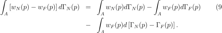
[image:13.612.134.516.224.281.2]Table 1: Counterfactual decompositions of the wage differential using natives as the reference group.
Counterfactually Remaining Wage Migrant
equalised para. differing para. differential effect
(1) p, α, µ, σ, λ, δ 32.022 6.825
(2) µ, σ p, α, λ, δ 30.096 3.747
(3) δ p, α, µ, σ, λ 28.973 1.954
(4) λ p, α, µ, σ, δ 34.029 10.032
(5) µ, σ, δ p, α, λ 27.423 -0.524
(6) α, µ, λ p, α, δ 31.694 6.300
(7) λ, δ p, α, µ, σ 30.459 4.328
(8) µ, σ, λ, δ p, α 28.758 1.610
(9) p, α µ, σ, λ, δ 4.904
(10) p, α, µ, σ λ, δ 1.932
(11) p, α, δ µ, σ, λ 0.750
(12) p, α, λ µ, σ, δ 7.814
(13) p, α, µ, σ, δ λ -1.842
(14) p, α, µ, σ, λ δ 4.400
(15) p, α, λ, δ µ, σ 2.741
Notes: Based on the DGP given in Appendix Table B.16, and the decompo-sition of equation (10). Rows 9+: the wage differential equals the migrant effect because the productivity distributions are the same.
tual migrant effect is, using (9),
Z
A
[wN(p|pN, αN, µN, σN, λN, δN)−wF(p|pF, αF, µN, σN, λF, δF)]dΓN(p) (10)
=
Z
A
wN(p|pN, αN, µN, σN, λN, δN)dΓN(p)−
Z
A
wF(p|pF, αF, µN, σN, λF, δF)dΓF(p)
−
Z
A
wF(p|pF, αF, µN, σN, λF, δF)d[ΓN(p)−ΓF(p)]
with Γi(p) = Γi(p|pi, αi) for i∈ {N, F}.
in row and experiment 2 is a shorthand forµF =µN andσF =σN. The residual
pa-rameters enumerated in column 2 constitute thus the sources of the remaining wage differences. In the first experiment, reported in row 1, no parameters are equalised, hence the reported results are based on actual wages (i.e. we use the actual wage decomposition (9)). In experiment 9 and later, we equalise the two parameters of the productivity distribution, p and α (Bartolucci (2013a) labels such differences in the productivity distribution parameters “segregation”). This nils the last term in equa-tion (10), so migrant effect and wage differential are equalised. In all experiments we use simulated data based on the DGP of Appendix Table B.16 but the results reported next are in line with our data-based empirical results for the comparative statics and policy experiments reported in Section 5.2.
The actual migrant effect of 6.8, reported in experiment 1, is substantial, about 21% of the wage differential. At the same time this implies that the largest con-tribution to the native-migrant wage gap is made by the differences between the productivity distributions. Turning to the drivers of the migrant effect, experiments 13-15 consider the marginal roles of δ, λ, and (µ, σ). Recalling that λF > λN
ex-plains the negative sign in experiment 13. Also note that δF > δN, and µF < µN
while σF = σN. Experiment 14 suggests that the difference in the separation rates
plays a large quantitative role in the determination of the migrant effect, the latter being 4.4; the complementary insight is that, by experiment 3, equalising the job separation rates reduces the migrant effect to 29% of its former size. The differences in mean reservation wages, considered in experiment 15, leads to a smaller migrant effect of 2.7. The joint effect of δ and (µ, σ), reported in experiment 12, equals 7.8, and is slightly larger than the sum of the two marginal effects. We defer discussing the policy implications of these results to Section 5.2 as these are similar to those based on our empirical results.
3. The Data
individuals not experiencing transitions during a calendar year is updated by means of an annual report. Hence, we are able to use a flow sample in our empirical analysis. Apart from wages, transfer payments, and spell markers, the dataset contains some standard demographic measures, including nationality, as well as occupation and firm markers. The education variable is not used since its problems, particularly in the migrant context, are well-known and skills are better measured by the occu-pation (see Fitzenberger et al. (2006) for a detailed discussion; we do not use the suggested imputations since the education variable for migrants, when observed, is likely to be of poor quality, as discussed in Br¨ucker and Jahn (2011, p. 296 point (ix)) and Lehmer and Ludsteck (2011, p. 900)). Wage records in the IABS are top coded at the social security contribution ceiling. However, this ceiling is not binding for our population of interest, namely individuals (natives and foreigners) in low and middle skill occupations. We use real wages in 1995 prices. The occupational information is provided in extensive (three digit codes) but non-standard form. We therefore map this coding into 10 major groups based on the International Standard Classification of Occupations (ISCO-88). The Data Appendix provides some details. Since immi-gration is known to be predominantly low skilled, we select from these 10 groups 3 low and middle skilled occupations, namely (1) unskilled blue-collar workers, (2) clerks and low-service workers, and (3) skilled blue-collar workers.
The data allows us to distinguish between three labour market states: employed, recipient of transfer payments (i.e. unemployment benefits, unemployment assis-tance and income maintenance during participation in training programs) and out of sample. Unfortunately, none of the two last categories corresponds exactly to the economic concept of unemployment. This issue is discussed in several studies, see e.g. Fitzenberger and Wilke (2010). For example, participants in a training program are transfer payment recipients despite being in employment (they are considered unemployed from an administrative point of view), while individuals that are regis-tered unemployed but are no longer entitled to receive benefits appear to be out of the labour force. Therefore, the dataset provides a representative sample of those employed and covered by the social security system, but somewhat mis-represents those in the state of unemployment. For our purposes, all individuals who are out of sample between two different spells are classified as unemployed, so only two labour market states are considered: unemployment and employment. The definition of unemployment used in our analysis is therefore somewhat broad: we assume that unemployment is proxied by non-employment, strictly speaking non-employment is an upper-bound for unemployment.
and not by place of birth. The data set does not report place of birth. Given this coding practice, some young foreign nationals might be born and raised in Germany. At the same time, ethnic Germans who immigrated from the former Soviet Union after the fall of the Berlin Wall will be classified as German, although they usually speak little German and have low skills. However, Dustmann et al. (2010) have argued that the former issue is ignorable, and we address the second by repeating the estimation using the subsample of individuals that were present in the data before the fall of the Berlin Wall, see the analysis in Section 4.5.3.
3.1. The Sample
[image:17.612.146.466.369.563.2]The data used in our empirical analysis is restricted to male full-time workers aged 25 to 55 years old residing in West-Germany (East Germany is excluded because of the peculiar transition processes taking place in the wake of unification). This sample is grouped into cells by occupation, nationality, and age. We define three age groups (25-30, 30-40, and 40-55) to proxy for potential experience. The aim of the grouping is to arrive at cells in which individuals are fairly homogeneous, and which are sufficiently large for the subsequent econometric investigation.
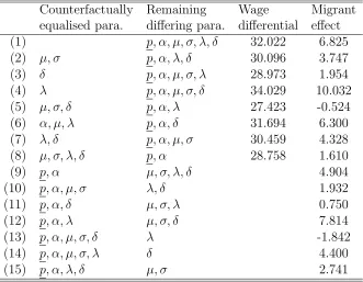
Table 2: Occupational Immobility: Share of Stayers by Segment
Age group Natives Foreigners
Unskilled 89.52% 88.27%
Twenties 85.72% 85.45%
Thirties 88.03% 88.56%
Fourtyplus 92.54% 92.38%
Clerks 90.06% 88.52%
Twenties 88.03% 87.33%
Thirties 87.44% 89.00%
Fourtyplus 91.82% 91.89%
Skilled 92.48% 92.56%
Twenties 90.35% 91.03%
Thirties 90.22% 92.43%
Fourtyplus 94.26% 95.25%
state, so that all durations are complete. The only exception is constituted by a small number of individuals who disappear from the dataset in the period 1995-2000, in which case their durations are considered censored. We note that the period 1995-2000 was a period of fairly stable growth (around 2%, with SD=.007) and un-employment (around 8%, with SD=.007). Focussing on this stable period reduces the scope for biases arising from asymmetric responses of natives and foreigners to the business cycle.
Foreigners in our sample are predominantly low skilled: 94% of the population of foreigners are included in our three occupational groups, while the corresponding number for natives is approximately 86%. The remainder occupational category is the highly skilled, which we have excluded because of their small share in the population of migrants (moreover, their earnings are excessively top-coded). Table 2 considers the occupational immobility by labour market segment. It is evident that occupational mobility is small, as most workers remain in the same class. This gives further support to our segmentation hypothesis, and such occupational immobility has also been found for other countries (e.g. by de Matos (2012) for Portugal).
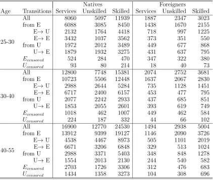
Table 3 summarises the labour market transitions for all nationality-age-occupation cells observed in our flow data. For both natives and foreigners, we observe many more transitions from employment than from unemployment. However, for natives, the majority of transitions from employment are to another job, whereas for the ma-jority of foreigners the destination is unemployment. Hence, in terms of the structural parameters, we expect higher separation rates for foreigners, δF > δN. The
dura-tion data for the unemployed, examined briefly in the next subsecdura-tion, suggests that foreigners exit more quickly, so that we expect λF > λN at least for this group.
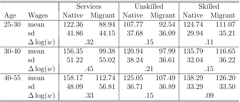
Turning to the wage data, Table 4 reports for each labour market segment the mean and standard deviation of wages (measured by daily gross wages in 1995 DM), as well as the average log wage gap, ∆ log(w)≡log(wN)−log(wF). Natives receive
substantially higher mean wages than foreigners across all occupation groups. The segment-specific raw average log wage gaps in our data range from .09 to .45. The overall log wage gap of .22 is in line with reports in the literature for Germany (e.g. Dustmann et al. (2010) report an unconditional average log wage gap of .23, Hirsch and Jahn (2012) report a gap of .2, while Lehmer and Ludsteck (2011) report predicted wage gaps ranging from .08 to .44). The three occupational groups can be partially ordered in terms of mean wages: mean wages for the skilled exceed those for the unskilled for all age groups and across nationalities. Foreign clerks and low-service workers assume an intermediate position, but mean wages of natives in this group can exceed those for skilled workers.
Table 3: Descriptives for the transition data.
Natives Foreigners
Age Transitions Services Unskilled Skilled Services Unskilled Skilled
25-30
All 8060 5097 11939 1887 2347 3023
from E 6088 3085 8450 1438 1670 2155
E→ U 2132 1764 4418 718 997 1225
E→ E 3432 1037 3562 373 351 550
from U 1972 2012 3489 449 677 868
U→ E 1879 1932 3275 431 637 795
Ecensored 524 284 470 347 322 380
Ucensored 93 80 214 18 40 73
30-40
All 12800 7748 15381 2074 2752 3681
from E 10723 5506 12448 1637 2067 2830
E→ U 2988 2644 5284 735 1128 1451
E→ E 6717 2400 6157 453 477 795
from U 2077 2242 2933 437 685 851
U→ E 1853 2055 2601 393 619 749
Ecensored 1018 462 1007 449 462 584
Ucensored 224 187 332 44 66 102
40-55
All 16900 12770 24530 1494 2938 5004
from E 13912 9399 19127 1146 2090 3726
E→ U 4538 4467 8973 505 1101 2019
E→ E 6671 3206 6848 329 513 1024
from U 2988 3371 5403 348 848 1278
U→ E 1554 2013 2130 244 540 582
Ecensored 2703 1726 3306 312 476 683
Ucensored 1434 1358 3273 104 308 696
Table 4: The average wage gap in the transition data by labour market segment.
Services Unskilled Skilled
Age Wages Native Migrant Native Migrant Native Migrant
25-30 mean 122.36 88.94 107.77 92.54 124.74 111.07
sd 41.86 44.15 37.68 36.09 29.94 35.21
∆ log(w) .32 .15 .11
30-40 mean 156.35 99.38 120.94 97.99 135.79 116.65
sd 51.22 55.02 38.24 36.61 32.04 36.22
∆ log(w) .45 .21 .15
40-55 mean 158.17 112.74 125.05 107.49 138.29 126.20
sd 48.09 56.81 36.71 36.89 33.29 33.50
∆ log(w) .33 .15 .09
Notes: ∆ log(w)≡log(wN)−log(wF). The overall log wage gap is .22. Wage dating: for transitions
from employment (E→ {U,E}), these are the last earned wages in this state, for transition out of
unemployment (U→E) these are the first wages earned in the new job.
kernel estimates of the realised wage densities (the solid lines refer to natives). The most pronounced distributional difference exist for the semi-skilled workers (clerks and service workers), and the differences persist across age groups. By contrast, for all other occupations, the differences decrease in age. The density estimates also exhibit “blips” in the far left tails of the wage densities. This bimodality leads to problems in the estimation of the model, manifesting themselves by the occurrence of spikes in the estimated productivity density. We overcome this issue by truncating the wage distributions at the 5% percentile, which is a common cut-off in the literature (see e.g. Bowlus (1997) or Flabbi (2010)). The estimation of the reservation wage distribution is, of coure, likely to be sensitive to the choice of the cut-off point. We therefore explore the robustness of our parameter estimates below in Section 4.5, and find that the frictional parameters are fairly stable, while µ increases usually somewhat as the truncation increases from 3% to 7%.
3.1.1. Reduced Form Estimates: The Importance of Unobservable Heterogeneity
Figure 2: Estimates of the density of accepted wages by labour market segments.
0 50 100 150 200 250 300
0.000 0.004 0.008 0.012 Accepted Wages Density
Clerks & Service Workers Age Group 25−30
0 50 100 150 200 250 300
0.000 0.004 0.008 0.012 Accepted Wages Density
Age Group 30−40
0 50 100 150 200 250 300
0.000 0.004 0.008 0.012 Accepted Wages Density
Age Group 40−55
0 50 100 150 200 250 300
0.000 0.004 0.008 0.012 Accepted Wages Density
Unskilled Blue Collar Workers Age Group 25−30
0 50 100 150 200 250 300
0.000 0.004 0.008 0.012 Accepted Wages Density
Age Group 30−40
0 50 100 150 200 250 300
0.000 0.004 0.008 0.012 Accepted Wages Density
Age Group 40−55
0 50 100 150 200 250 300
0.000 0.005 0.010 0.015 Accepted Wages Density
Skilled Blue Collar Workers Age Group 25−30
0 50 100 150 200 250 300
0.000 0.005 0.010 0.015 Accepted Wages Density
Age Group 30−40
0 50 100 150 200 250 300
0.000 0.005 0.010 0.015 Accepted Wages Density
Age Group 40−55
Notes: Natives (solid lines) v. foreigners (dashed lines).
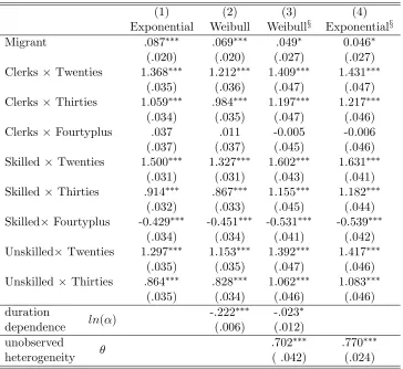
the conditional unemployment durations in the structural model are exponential with parameterλF¯(b) and the marginal durations are a mixture of such exponentials, we first estimate an exponential PH model, and then allow for duration dependence by estimating a Weibull specification. As the latter confounds dynamic sorting driven by unobservable heterogeneity and genuine duration dependence (see e.g. van den Berg (2001)), we then estimate MPH models using the common gamma frailty (as-sumed to be independent of the covariates). Note, however, that these reduced-form parameters do not identify the parameters of the structural model as the former are complicated functions of the latter. In all models we condition on interactions between age and occupational groups in order to mirror our subsequent structural analysis of the corresponding labour market segments.
to be caused by dynamic sorting: once unobservable heterogeneity is controlled for, the Weibull parameter does not differ statistically from 1. Hence Weibull and ex-ponential MPH models yield similar coefficient estimates. This inferred absence of duration dependence is consistent with the structural model, as it cannot generate genuine duration dependence but does yield dynamic sorting through unobserved heterogeneity in reservation wages.
Table 5: Reduced-form unemployment duration models
(1) (2) (3) (4) Exponential Weibull Weibull§ Exponential§
Migrant .087∗∗∗ .069∗∗∗ .049∗ 0.046∗ (.020) (.020) (.027) (.027) Clerks ×Twenties 1.368∗∗∗ 1.212∗∗∗ 1.409∗∗∗ 1.431∗∗∗
(.035) (.036) (.047) (.047) Clerks ×Thirties 1.059∗∗∗ .984∗∗∗ 1.197∗∗∗ 1.217∗∗∗
(.034) (.035) (.047) (.046) Clerks ×Fourtyplus .037 .011 -0.005 -0.006 (.037) (.037) (.045) (.046) Skilled ×Twenties 1.500∗∗∗ 1.327∗∗∗ 1.602∗∗∗ 1.631∗∗∗
(.031) (.031) (.043) (.041) Skilled ×Thirties .914∗∗∗ .867∗∗∗ 1.155∗∗∗ 1.182∗∗∗
(.032) (.033) (.045) (.044) Skilled×Fourtyplus -0.429∗∗∗ -0.451∗∗∗ -0.531∗∗∗ -0.539∗∗∗
(.034) (.034) (.041) (.042) Unskilled×Twenties 1.297∗∗∗ 1.153∗∗∗ 1.392∗∗∗ 1.417∗∗∗
(.035) (.035) (.047) (.046) Unskilled × Thirties .864∗∗∗ .828∗∗∗ 1.062∗∗∗ 1.083∗∗∗
(.035) (.034) (.046) (.046) duration
ln(α) -.222
∗∗∗ -.023∗
dependence (.006) (.012) unobserved
θ .702
∗∗∗ .770∗∗∗
4. Estimation Results
[image:23.612.99.542.245.442.2]We proceed to estimate the structural parameters of the model, i.e. the job offer arrival rate,λ, the match destruction rate, δ, and the parameters of the distribution of workers’ reservation values, (µ, σ), as well as the density of firms’ productivity in each segment. Each occupation group is considered in turn, and we segment for each occupation the labour market further by age and nationality. The average migrant effects and the wage decompositions are then quantified in detail in Section 5 below.
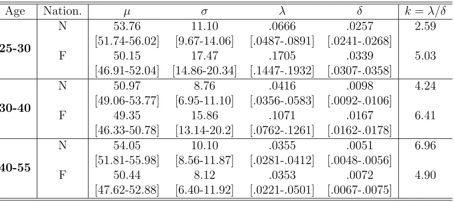
Table 6: Structural parameter estimates: Unskilled blue collar workers
Age Nation. µ σ λ δ k =λ/δ
25-30
N 53.76 11.10 .0666 .0257 2.59
[51.74-56.02] [9.67-14.06] [.0487-.0891] [.0241-.0268]
F 50.15 17.47 .1705 .0339 5.03
[46.91-52.04] [14.86-20.34] [.1447-.1932] [.0307-.0358]
30-40
N 50.97 8.76 .0416 .0098 4.24
[49.06-53.77] [6.95-11.10] [.0356-.0583] [.0092-.0106]
F 49.35 15.86 .1071 .0167 6.41
[46.33-50.78] [13.14-20.2] [.0762-.1261] [.0162-.0178]
40-55
N 54.05 10.10 .0355 .0051 6.96
[51.81-55.98] [8.56-11.87] [.0281-.0412] [.0048-.0056]
F 50.44 8.12 .0353 .0072 4.90
[47.62-52.88] [6.40-11.92] [.0221-.0501] [.0067-.0075]
Notes: In brackets: the 2.5% and 97.5% percentiles of the bootstrap distribution.
4.1. Unskilled Blue Collar Workers
Table 6 reports the results. Across all three age groups, the labour turnover parameters of migrants exceed those of natives, ˆδF > ˆδN and ˆλF > λˆN. Migrants
experience job separations more often, but this is partially compensated by them also finding new jobs more quickly. All job turnover parameters fall in age. Across age groups and nationality, transitions into new jobs happen more quickly than tran-sitions into unemployment, ˆλ > ˆδ. Foreigners have slightly lower mean reservation wages, ˆµF < µˆN, but confidence intervals overlap. The estimates are fairly stable
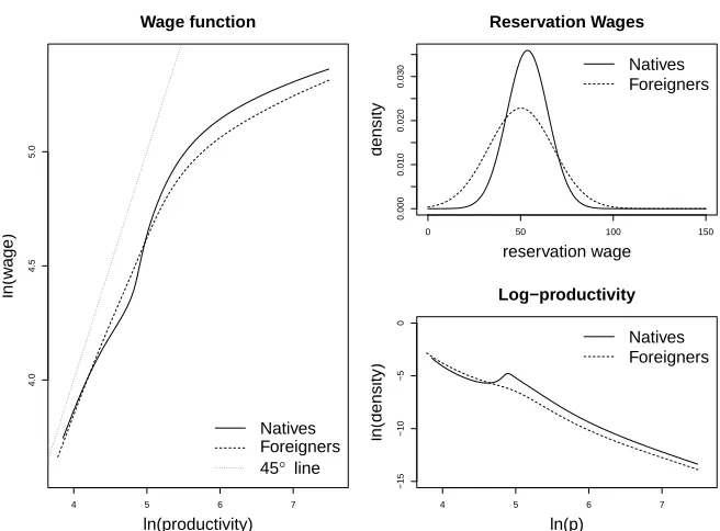
In Figure 3 we consider some implications of the estimated model for the young. Panel A plots the wage offer functions, panel B the reservation wage density, whilst panel C plots the estimated productivity densities10. It is evident that the produc-tivity densities for both groups are well approximated by a Pareto density. The slopes for sufficiently high productivities are very similar. Turning to wage offers (panel A), for low productivities foreigners do not do worse than natives, while for log productivities above 5 natives receive better wage offers. Overall, the figure sug-gests a positive but small migrant effect, and this is confirmed by our quantifications reported in Section 5.
Figure 3: Unskilled blue collar workers aged 25-30.
4 5 6 7
4.0
4.5
5.0
Wage function
ln(productivity)
ln(w
age)
Natives Foreigners 45° line
0 50 100 150
0.000
0.010
0.020
0.030
Reservation Wages
reservation wage
density
Natives Foreigners
4 5 6 7
−15
−10
−5
0
Log−productivity
ln(p)
ln(density)
Natives Foreigners
4.2. Clerks and Low-Service Workers
Table 7 reports the results for this occupational group, for which we observed in Table 4 the largest average wage gap. As before, job separation rates for foreigners exceed those of natives, decline in age, and are smaller than job offer arrival rates.
10
These are obtained as follows. Given the parameter estimates and kernel estimate of the
realised wage density, the unemployment rateuis estimated using equation (4), and the wage offer
Table 7: Structural parameter estimates: Clerks & service workers
Age Nation. µ σ λ δ k =λ/δ
25-30
N 65.60 14.39 .0984 .0194 5.07
[61.92-66.53] [11.61-15.8] [.0697-.0836] [.0189-.0199]
F 36.09 13.65 .0701 .0272 2.58
[30.88-41.69] [8.6-17.17] [.0624-.0886] [.0259-.0284]
30-40
N 72.66 9.42 .0423 .0073 5.79
[68.41-75.12] [7.54-10.39] [.0355-.0530] [.0071-.0076]
F 43.27 7.40 .0593 .0157 3.77
[40.88-45.62] [6.41-9.57] [.0478-.0703] [.0151-.0162]
40-55
N 73.07 7.92 .0698 .0035 19.94
[70.51-75.12] [7.07-9.16] [.0603-.0841] [.0031-.0037]
F 49.04 6.86 .0759 .0077 9.86
[46.38-51.94] [5.22-8.41] [.0565-.0911] [.0072-.0081]
Notes: As for Table 6.
Except for the young, the transition rates of foreigners exceed those of natives. But unlike the case of the unskilled, differences in mean reservation wages are substan-tial: foreigners are substantially less demanding, on average, than natives. These means increase in age. Figure 4 panel C suggests that productivities are again well approximated by a Pareto form, and panel A suggests that the maximal migrant effect is substantial.
4.3. Skilled Blue-Collar Workers
For the skilled blue-collar workers, the by now familiar pattern emerges too, as is evident from Table 8: both turnover parameters are higher for migrants, and decline in age. As regards mean reservation wages, foreigners are less demanding than natives, but the gap is not as wide as for clerks and service workers, and it declines in age. Focussing on the young in Figure 5, productivities are Pareto like. The migrant effect, captured in Panel A, is modest.
4.4. General Discussion
Figure 4: Clerks and service workers aged 25-30.
4 5 6 7 8
3.5
4.0
4.5
5.0
5.5
Wage function
ln(productivity)
ln(w
age)
Natives Foreigners 45° line
0 50 100 150
0.000
0.010
0.020
0.030
Reservation Wages
reservation wage
density
Natives Foreigners
4 5 6 7 8
−15
−10
−5
0
Log−productivity
ln(p)
ln(density)
Natives Foreigners
Table 8: Structural parameter estimates: Skilled blue collar workers
Age Nation. µ σ λ δ k=λ/δ
25-30
N 81.15 4.52 .0801 .0158 5.07
[77.64-83.97] [3.81-6.59] [.0684-.0911] [.0121-.0179]
F 66.38 14.05 .1067 .0225 4.74
[62.88-69.04] [11.88-17.32] [0.955-0.1182] [.0170-.0268]
30-40
N 76.68 8.85 .0698 .0068 10.26
[73.82-77.90] [7.69-9.71] [.0621-.0760] [.0063-.0071]
F 69.30 8.06 .0866 .0124 6.98
[65.57-72.05] [7.34-9.16] [.0681-.0946] [.0119-.0127]
40-55
N 79.71 6.44 .0408 .0035 11.66
[77.18-80.94] [5.62-7.01] [.0343-.0478] [.0033-.0036]
F 75.05 7.33 .0449 .0049 9.16
[71.48-78.24] [6.51-8.70] [.0325-.0512] [.0045-.0051]
[image:26.612.97.547.424.619.2]Figure 5: Skilled blue collar workers aged 25-30.
4 5 6 7 8
4.0
4.5
5.0
5.5
Wage function
ln(productivity)
ln(w
age)
Natives Foreigners 45° line
0 50 100 150
0.00
0.02
0.04
0.06
0.08
Reservation Wages
reservation wage
density
Natives Foreigners
4 5 6 7 8
−15
−10
−5
0
Log−productivity
ln(p)
ln(density)
that migrants in Germany are much more likely than natives to work on temporary contracts. The findings are also consistent with the other dimensions of segrega-tion extensively documented in Glitz (2012). Across all segments and nasegrega-tionality, transitions into new jobs happen more quickly than transitions into unemployment. Overall, search frictions, as measured by (λ/δ)−1, are of the same order of magni-tude across all occupational groups, decrease in age (except for unskilled foreigners in which case they are stable), and are larger for foreigners than for natives for the skilled and clerks and service workers. Thus, the higher job offer arrival rate for foreigners cannot compensate for their higher job separation rates. As regards the reservation wage distribution, across all segments there are some workers with high reservation wages who turn down new job offers when wage offers are too low.11 Mi-grant workers are on average less demanding than natives. Firm productivities are well approximated by Pareto forms. However, migrants receive wage offers that are lower than for natives who have the same productivity. This migrant effect is the largest for clerks and service workers, and small for unskilled workers. The drivers of the migrant effect are the subject of Section 5.
4.5. Robustness Checks 4.5.1. Return Migration
A concern for our estimates in the migrant segments might be the effect of return migration, when such returnees leave Germany out of employment. In order to investigate the sensitivity of our estimates to this issue, we consider restricted samples of migrants who should, in principle, be available for work after their employment transition, by requiring foreigners to be observable in the data 6 months after their transition. This restriction leads to a net dropout of foreigners (relative to that of
11
These results differ from estimates for Netherlands (van den Berg and Ridder (1998)) and France (Bontemps et al. (1999)) since both countries have a binding legal minimum wage. Similar
to these studies, however, we observe that job separation parameterδ is approximately one order
of magnitude smaller than the estimated job offer arrival rate λ. Our results are comparable to
those reported by Bartolucci (2013a) for Germany obtained from a different empirical search model applied to a different market segmentation. For low qualified male workers in the manufacturing
sector he reports a job separation rate of .03 and a job offer arrival rate of .3. Our estimates ofδ
natives) across segments between 7.7% and 15.3%.12 Table 9 juxtaposes the estimates for these restricted samples (labelled noRetMig) to our unrestricted estimates. We find that most parameter estimates remain relatively stable (the occasional fall in ˆ
[image:29.612.135.478.210.497.2]σ reflects the extent to which the sample restriction increases the homogeneity of the group; the more homogeneous the sample, the smaller the estimated reservation wage dispersion).
Table 9: Sensitivity analysis - the effect of excluding return migrants
Occupation Age Group µ σ λ δ
Unskilled
25-30 full 50.15 17.47 0.1705 0.0339
noRetMig 49.88 10.14 0.1207 0.0433
30-40 full 49.35 15.86 0.1071 0.0167
noRetMig 50.65 8.53 0.0588 0.0219
40-55 full 50.44 8.12 0.0353 0.0072
noRetMig 48.53 3.28 0.0495 0.0087
Skilled
25-30 full 66.38 14.05 0.1067 0.0225
noRetMig 65.00 9.05 0.0871 0.0281
30-40 full 69.30 8.06 0.0866 0.0124
noRetMig 68.72 5.86 0.0660 0.0142
40-55 full 75.05 7.33 0.0449 0.0049
noRetMig 62.74 7.44 0.0379 0.0058
25-30 full 36.09 13.65 0.0701 0.0272
noRetMig 37.84 11.37 0.0749 0.0344 Clerks
30-40 full 43.27 7.40 0.0593 0.0157
& Services noRetMig 45.11 9.09 0.0689 0.0201
40-55 full 49.04 6.86 0.0759 0.0077
noRetMig 48.23 5.39 0.1036 0.0098
4.5.2. The effect of truncating the wage distribution
Our samples have been truncated at 5% at the left tail of the wage distribution, a common cut-off in the literature. Here, we examine the sensitivity of our estimates to varying the cut-off from 3% to 7%. Table 10 reports the results. Across all segments,
12
Table 10: Sensitivity analysis - the effects of truncation
Occupation Age Trunc. Foreigners Natives
µ σ λ δ µ σ λ δ
Unskilled
25-30
3% 45.31 19.68 .1698 .0344 42.77 15.85 .0603 .0256 5% 50.15 17.47 .1705 .0339 53.76 11.10 .0666 .0257 7% 54.47 15.18 .1593 .0333 56.72 9.53 .0783 .0254
30-40
3% 47.89 16.51 .1215 .0167 38.62 11.64 .0321 .0099 5% 49.35 15.86 .1071 .0167 50.97 8.76 .0416 .0098 7% 55.62 12.56 .1000 .0162 57.53 9.10 .0306 .0095
40-55
3% 40.18 3.86 .0435 .0074 38.62 11.64 .0321 .0099 5% 50.44 8.12 .0353 .0072 54.05 10.10 .0355 .0051 7% 52.83 7.64 .0298 .0071 53.87 14.73 .0276 .0049
Skilled
25-30
3% 57.41 18.69 .0915 .0229 72.78 9.66 .0611 .0162 5% 66.38 14.05 .1067 .0225 81.15 4.52 .0801 .0158 7% 71.79 10.38 .1061 .0219 82.65 3.72 .0729 .0154
30-40
3% 63.53 12.14 .0695 .0127 73.51 9.44 .0798 .0069 5% 69.30 8.06 .0866 .0124 76.68 8.85 .0698 .0068 7% 72.36 6.56 .0579 .0121 87.08 4.58 .0612 .0064
40-55
3% 67.90 7.57 .0557 .0045 69.17 8.12 .0407 .0036 5% 75.05 7.33 .0449 .0049 79.71 6.44 .0408 .0035 7% 77.32 5.81 .0392 .0045 83.31 5.40 .0583 .0035
25-30
3% 35.43 14.04 .0628 .0269 58.30 18.68 .1113 .0198 5% 36.09 13.65 .0701 .0272 65.60 14.39 .0984 .0194 7% 35.44 14.04 .0628 .0269 68.11 13.14 .0953 .0191
30-40
3% 41.98 7.83 .0608 .0156 62.80 15.13 .0555 .0075
Clerks 5% 43.27 7.40 .0593 .0157 72.66 9.42 .0423 .0073
& Services 7% 47.34 5.79 .0464 .0154 78.16 5.92 .0490 .0072
40-55
the frictional parameters δ and λ are very stable. An increase in the truncation is expected to lead to an increase in the estimated mean reservation wage. This increase, however, turns out to be typically very modest. We conclude that our estimates are robust.
[image:31.612.150.463.210.407.2]4.5.3. Ethnic German Immigrants
Table 11: Native workers: full and restricted sample results
Occupation Age Group µ σ λ δ
Unskilled
30-40 all 50.97 8.76 .0416 .0098
pre ’88 48.46 5.22 .0362 .0090
40-55 all 54.05 10.10 .0355 .0051
pre ’88 51.95 6.66 .0203 .0046
Skilled
30-40 all 76.68 8.85 .0698 .0068
pre ’88 88.53 2.78 .0700 .0060
40-55 all 79.71 6.44 .0408 .0035
pre ’88 81.34 7.51 .0407 .0032
Clerks 30-40 all 72.66 9.42 .0423 .0073
& Services pre ’88 71.11 9.12 .0496 .0067
40-55 all 73.07 7.92 .0698 .0035
pre ’88 72.66 8.93 .0413 .0033
Notes: “all” refers to the full sample of native workers, “pre ’88” to the sample of natives observed before 1988.
and the subsample, which suggests that the presence of ethnic Germans has only little effect on the estimates of the structural parameters for natives.
5. Migrant Effects and Wage Decompositions
We proceed to examine actual and counterfactual decompositions of the wage differential by considering the scenarios of Section 2.4.1. The discussion there has highlighted the importance of the productivity distribution, and we operationalise the decomposition as follows.
5.1. Calibration Details
Our estimation has yielded, given the (estimate of the) actual wage distributionG, the estimated wage offer functionswe
i(p|ˆλ,δ,ˆ µ,ˆ σˆ). Given the Pareto-like productivity
distributions, we calibrate wage offer functions wi(p|λ,ˆ δ,ˆ µ,ˆ σ, p, αˆ ) based on Pareto
productivity distributions by minimising the integrated absolute deviations between
we
[image:32.612.119.495.354.471.2]i(p|.) and wi(p|., p, α). Table 12 reports the calibrated parameters.13
Table 12: Calibrated parameters of the Pareto productivity distribution.
Age Group Nationality Unskilled Skilled Clerks
p α p α p α
25-30 Natives 79.789 2.511 81.282 3.172 67.677 2.449 Foreigners 47.632 2.205 51.010 2.146 43.053 1.468 30-40 Natives 84.343 2.894 71.212 3.076 104.849 3.096 Foreigners 57.071 2.611 61.414 2.661 41.818 1.463 40-55 Natives 70.263 2.842 69.293 3.045 72.222 3.197 Foreigners 70.202 2.833 63.838 2.896 34.545 1.738
Figure 6 illustrates these calibrations for young workers in the three occupations, as well as the counterfactual experiment of improving the job turnover situation of foreigners by lowering their job separation rate to those of natives,δF ≡δN. The first
two columns of the figure show the close match between we(p) (which we have seen
before in Figure 3) andw(p). Column three depicts the calibrated wage offerswN(p)
(solid line) andwF(p) (dashed line), as well as the counterfactualwF(p|.,δˆN) (dotted
13
line). The reduction in the separation rate for foreigners from ˆδF to ˆδN ‘rotates’
the wage offer curve up: for lower productivities, the improvement is negligible, but for very high productivities foreigners receive wage offers equal to or better than those for natives. This results in the improvement in the density of accepted wages depicted in the fourth column of the figure.
5.2. Results
Tables 13 to 15 report by age group the average migrant effect (row 1), as well as the results of the counterfactual experiments which follow the structure of Table 1. We can anticipate the qualitative results of these experiments based on numerical comparative statics exercises which show (for the set of parameters considered) that wage offers increase in the job offer arrival rate λ as search frictions decrease, and, contrariwise, decrease in the job separation rate δ as search frictions increase. Of course, as k = λ/δ → ∞ and search frictions disappear, by eq. (3), wage offers converge to the competitive wage. Wage offers increase in the mean reservation wage
µ, since by the reservation wage property of job search only sufficiently high wage offers are accepted out of unemployment, but the effect of σ is ambiguous. Since we found that job separation rates for foreigners always exceed those of natives, setting
δF =δN increases their wage offers, which implies a reduction both of the wage gap
and the migrant effect. Similarly, we found that λF > λN (except for young clerks
and service workers), so reducing the foreigners’ job offer arrival rate to that of natives reduces their wage offers, which implies an increase both in the wage gap and the migrant effect. As regards reservation wages, we found that foreigners are on average less demanding than natives, but the overall effect of the joint experiment involving (µ, σ) is ambiguous given the ambiguous effect ofσ. All these qualitative effects are observed in the results tables (experiments (1)-(4)). The principal objective of the tables is then to quantify the impacts in order to understand the principal drivers of the migrant effect.
Ludsteck (2011) report a range from 4 to 17%) or complementary approaches (Hirsch and Jahn (2012) report 6% while Bartolucci (2013b) suggests discrimination effects ranging between 7 and 17%). The observed difference between the wage differential and the migrant effect also implies that the largest part of the native-migrant wage gap is explained by differences in the productivity distribution, which is confirmed in experiment (9) by the drop in the wage gap (which now equals the migrant effect by construction). Policy interventions that seek to reduce the productivity gap will thus reduce the wage gap. We turn to the various experiments, highlighting the role of search frictions.
Consider first the role of the mean reservation wage µ (experiment (2)). The gap in mean reservation wages is the largest for clerks and service workers whilst the dispersion parameters are fairly similar. Raising then the foreigners’ mean reser-vation wages shows that the substantial migrant effect for this occupational group is reduced to between 41% and 61% of its former level. For the skilled, we only observe a significant gap in mean reservation wages for the young, and an equali-sation of (µ, σ) reduces the migrant effect to 48% of its former level. For the other age groups, and for the unskilled, differences in µ between natives and foreigners are either small or negligible, so equalisations have little effect. Once productivity differences have been eliminated, a comparison between experiments (9) and (10) shows that for clerks and service workers, the relative improvement in the migrant effect due to the additional equalisation of (µ, σ) is slightly larger (the migrant effect is now between 20% and 30% of the level generated in experiment (9)). Turning to the policy implications, although foreigners are on average less demanding than na-tives, we believe that foreigners’ reservation wages should be less a concern for policy interventions which are migrant-centred (as emphasised by recent policy debates in the EU, e.g. EUCommission (2012, p. 28)) and seek to reduce the migrant effect. Nor would any migrant-targeted benefit increase be politically feasible in the light of the debate about welfare magnets.
By the same token, job arrival rates for foreigners typically exceed those of natives, and thus should equally be of little policy concern. In fact, the experiments (4) show that reducing this rate to that of natives only substantially increases the migrant effect for the unskilled in the two first age groups; for all other groups the induced increase in the migrant effect is fairly small. This is also in line with the observation that λ falls in age for the unskilled and skilled.
is scope for migrant-centred policy interventions that seek to reduce their search frictions, such as improving migrants’ employment protection. This scope, however, decreases in age, as δ falls in age across all occupational groups. Reducing the foreigners’ job separation rates to that of natives has the largest absolute impact for clerks and service workers, followed by the skilled. For the unskilled, the migrant effect is already fairly small, and an equalisation ofδ reduces the remainder further.
6. Conclusion
The use of the structural empirical general equilibrium search model with on-the-job search has enabled us to disentangle the role of various unobservables for the explanation of wage differentials between migrants and natives. In particular, we have examined differences in search frictions, reservation wages, and productivities in segments of the labour market defined by occupation, age, and nationality using a large scale German administrative dataset. The resulting decompositions of the actual and counterfactual wage differential quantify the marginal and joint roles of the various factors.
Acknowledgements
Financial support from the NORFACE research programme on Migration in Eu-rope -Social, Economic, Cultural and Policy Dynamics is gratefully acknowledged. Thanks to Norface conference participants, especially G. Peri and C. Dustmann for comments, as well as N. Theodoropoulos. We also wish to thank our three referees whose detailed and very constructive comments have helped to improve the paper.