Sparse Array Design for Wideband Beamforming with Reduced Complexity in Tapped Delay-lines

Reduced Complexity in Tapped Delay-lines

.

White Rose Research Online URL for this paper:

http://eprints.whiterose.ac.uk/85451/

Version: Accepted Version

Article:

Liu, W. and Hawes, M.B. (2014) Sparse Array Design for Wideband Beamforming with

Reduced Complexity in Tapped Delay-lines. IEEE Transactions on Audio, Speech and

Language Processing, 22 (8). pp. 1236-1247. ISSN 1558-7916

https://doi.org/10.1109/TASLP.2014.2327298

[email protected] https://eprints.whiterose.ac.uk/ Reuse

Unless indicated otherwise, fulltext items are protected by copyright with all rights reserved. The copyright exception in section 29 of the Copyright, Designs and Patents Act 1988 allows the making of a single copy solely for the purpose of non-commercial research or private study within the limits of fair dealing. The publisher or other rights-holder may allow further reproduction and re-use of this version - refer to the White Rose Research Online record for this item. Where records identify the publisher as the copyright holder, users can verify any specific terms of use on the publisher’s website.

Takedown

If you consider content in White Rose Research Online to be in breach of UK law, please notify us by

Sparse Array Design for Wideband

Beamforming with Reduced Complexity in

Tapped Delay-lines

Matthew B. Hawes and Wei Liu Communications Research Group

Department of Electronic and Electrical Engineering University of Sheffield, UK

{elp10mbh, w.liu}@sheffield.ac.uk

Abstract—Sparse wideband array design for sensor location optimisation is highly nonlinear and it is traditionally solved by genetic algorithms (GAs) or other similar optimization methods. This is an extremely time-consuming process and an optimum solution is not always guaranteed. In this work, this problem is studied from the viewpoint of compressive sensing (CS). Although there have been CS-based methods proposed for the design of sparse narrowband arrays, its extension to the wideband case is not straightforward, as there are multiple coefficients associated with each sensor and they have to be simultaneously minimised in order to discard the corresponding sensor locations. At first, sensor location optimisation for both general wideband beamforming and frequency invariant beamforming is consid-ered. Then, sparsity in the tapped delay-line (TDL) coefficients associated with each sensor is considered in order to reduce the implementation complexity of each TDL. Finally, design of robust wideband arrays against norm-bounded steering vector errors is addressed. Design examples are provided to verify the effectiveness of the proposed methods, with comparisons drawn with a GA-based design method.

Index Terms—Sparse array, frequency invariant beamform-ing, wideband beamformbeamform-ing, robust beamformbeamform-ing, compressive sensing, implementation complexity.

I. INTRODUCTION

Wideband beamforming has been studied extensively in the past [1], [2], [3], [4], [5], [6]. It is well-known that in order to avoid the spatial aliasing problem for uniform linear arrays (ULAs), the adjacent sensor spacing has to be less than half of the minimum operating wavelength corresponding to the highest frequency of the signal of interest. This can be problematic when considering arrays with a large aperture size, due to the cost associated with the number of sensors required. As a result, sparse arrays, which allow adjacent sensor sep-arations greater than half a wavelength while still avoiding grating lobes due to the randomness of sensor locations, are a desirable alternative [7]. Moreover, even with the same number of sensors and a similar aperture size, the nonuniform nature of a sparse array also provides more degrees of freedom to achieve a better beam response.

However, the unpredictable sidelobe behaviour associated with sparse arrays means some optimisation of sensor loca-tions is required to reach an acceptable performance level. Var-ious nonlinear methods have been used to achieve this required optimisation. For example, Genetic Algorithms (GAs) [8], [9], [10], [11], [12], [13], Simulated Annealing (SA) [14], [15]. In

Copyright (c) 2014 IEEE. Personal use of this material is permitted. However, permission to use this material for any other purposes must be obtained from the IEEE by sending a request to [email protected].

particular, in [16], the wideband sparse array design problem is studied using an SA-based approach which can result to either a frequency invariant response or a maximum directivity one while controlling the sidelobe level and without the need of setting a desired response in advance. The disadvantage of these types of methods are the potentially extremely long computation times and the possibility of convergence to a non-optimal solution.

Recently, the area of compressive sensing (CS) has been explored [17], and CS-based methods have been proposed in the design of narrowband sparse arrays [18], [19], [20], [21], [22], [23], [24], [25]. CS theory tells us that if certain conditions are met it is possible to recover some signals from fewer measurements than are used by traditional methods. This can then form the basis of sparse array design methods by trying to attain an exact, or almost exact, match to a desired response while using as few sensors as possible. This is achieved by minimising the l1 norm of the weight coeffi-cients, subject to the error between the desired and designed responses being below a predefined level. Further work has also shown that it is possible to improve the sparseness of a solution by considering a reweightedl1minimisation problem [26], [27], [28]. The aim of these methods is to bring the minimisation of the l1 norm of the weight coefficients closer to that of the minimisation of thel0norm, by solving a series of reweighted l1 minimisations, where locations with small weight coefficients are more heavily penalised than locations with large weight coefficients.

It is not straightforward to extend the design to the wideband case, as there are tapped delay-lines (TDLs) or FIR/IIR filters associated with each received wideband signal, and for a wideband array to be sparse all coefficients along the TDL associated with an individual sensor have to be equal or very close to zero. Therefore, it is not sufficient to simply minimize the l1 norm of the weight coefficients. Instead all the weight coefficients along a TDL have to be simultaneously minimized. In order to achieve this, a method similar to the technique employed in complex-valued l1 norm minimization [29], is proposed in this paper, which is a further expansion of the idea presented in [30] by the same authors. As in the case with the reweighted l1 minimisation method for narrowband array design, it is possible to use a reweighted scheme for the wideband method as well. This involves the reweighting terms being applied to the weight coefficients in the reformulated wideband problem.

A further contribution in this work is the design of sparse frequency invariant beamformers (FIBs) using the CS-based approach. FIB design has been studied in the areas of fixed [31], [32], [33], [34], and adaptive [35], beamforming. Both use the idea of response variation (RV) to account for the difference in response at each frequency to that at the reference frequency in the design process. In this work the RV will be added as a constraint to the reformulated wideband CS problem in an attempt to obtain a sparse FIB.

have been studied in the FIR filter design area [36], [37], [38]. In this work we propose looking at this problem from the view point of CS and to combine it with the traditional problem of finding the minimum number of active sensor locations, with two methods being proposed. Firstly, a fixed set of sensor locations can be found using one of our proposed wideband CS methods. The final coefficients for these fixed locations can then be found by solving a second l1 minimisation of the weight coefficients. Alternatively, the sparsity in locations and in coefficients along a TDL can be simultaneously maximised. To do this the cost function at the start of the wideband CS reformulation has to be altered. In both cases a reweighted scheme can be derived.

Moreover, one practical issue in the design of wideband ar-rays is the steering vector error caused by model perturbations such as sensor location errors and individual sensor response discrepancies. Many methods have been proposed for robust design of such arrays, such as constraining the white noise gain [39], [40], using worst-case performance optimisation [41] or considering the probability density functions of the sensor characteristics [16]. In this work we use an extra constraint to limit the effect of norm-bounded steering vector errors [23], [42], which ensures the maximum possible change in array response remains below a predetermined acceptable level, therefore allowing a robust response.

The remainder of this paper is structured as follows. Sec. II gives details of the proposed CS-based design methods for location sparsity, which includes the array model in II-A, the proposed standard CS method in II-B, and derivation of the frequency invariant (FI) constraint for CS in II-C, with II-D showing how the problem can be altered to a reweighted CS problem. Details of two design methods for a lower complexity TDL are shown in Sec. III, with Sec. IV giving details of a constraint that ensure robustness to steering vector errors. Finally, design examples are provided in Sec. V and conclusions drawn in Sec. VI.

II. PROPOSEDWIDEBANDARRAYDESIGNS FOR

LOCATIONSPARSITY

A. Wideband Array Model

A general linear array structure for wideband beamforming with a TDL length J is shown in Fig. 1, where Ts is the

sampling period or temporal delay between adjacent signal samples [2]. We assume that all of the sensors are omnidirec-tional with the same response, and the signals impinge upon the array from the far field. The beamformer output y[n] is a linear combination of differently delayed versions of the received array signalsxm[n],m= 0,· · ·, M−1. The distance

from the zeroth sensor to the subsequent sensor is denoted by

dmform= 0,· · · , M−1, withd0= 0. Fig. 1 also shows an incident signal arriving at an angle θ.

The steering vector of the array as a function of the normalized frequency Ω =ωTs and the arrival angleθ is

s(Ω, θ) = [1,· · ·, e−jΩ(J−1)_{, e}−jΩµ1cos(θ)_,

e−jΩ(µ₁cos(θ)+1)

,· · ·, e−jΩ(µ₁cos(θ)+(J−1))

,

· · · , e−jΩ(µM₋₁cos(θ)+(J−1))_]T _,

(1)

[n]

s Ts

w

w

w

T_s T_s

x0[n]

M−1 d

w

w

w

y[n] θ

θ

M−1,0 xM−1

T

Fig. 1. A general wideband beamforming structure with a TDL lengthJ.

whereµm=_cTdms form= 0,1,· · ·, M−1and{·}

T _indicates

transpose operation.

The response of the array is then given by

P(Ω, θ) =wHs(Ω, θ), (2)

wherewH is the Hermitian transpose of the weight vector of the array, given by

w = [wT₀ wT₁ ... wT_M−1]T (3)

wm = [wm,0 wm,1 ... wm,J−1]T . (4)

B. Sparse Wideband Array Design via Compressive Sensing

CS has been employed in the design of sparse narrow-band arrays by trying to match the array’s response to a desired/reference one, Pr(Ω, θ). Extending the design to the

wideband case, we first consider Fig. 1 as being a grid of potential active sensor locations. In this instance, dM−1 is the maximum aperture of the array and the values ofdm, for

m= 1,2, . . . , M−2, are selected to give a uniform grid, with

M being a large enough number to cover all potential locations of the sensors. Sparseness is then introduced by selecting the set of weight coefficients to give as few active locations as possible, while still giving a designed response that is close to the desired one.

In the first instance, this problem could be formulated as

min||w||0 subject to ||p_r−wHS||2≤α , (5)

where ||w||0 is the number of nonzero coefficients in w, p_r

is the vector holding the desired beam response at sampled frequency points Ωk and angle θl, k = 0,· · ·, K −1, l =

0,· · ·, L−1,Sis the matrix composed of the steering vectors at the corresponding frequency Ωk and angle θl, αplaces a

limit on the allowed difference between desired and designed responses, and||.||2 denotes thel2 norm.

In detail,p_r andSare respectively given by

p_r = [Pr(Ω0, θ0),· · ·, Pr(Ω0, θL−1), Pr(Ω1, θ0), · · ·, Pr(Ω1, θL−1),· · ·, Pr(ΩK−1, θL−1)] (6)

and

S = [s(Ω0, θ0),· · ·,s(Ω0, θL−1),s(Ω1, θ0), · · ·,s(Ω1, θL−1),· · · ,s(ΩK−1, θL−1)]. (7)

Here the desired responsePr(Ω, θ)can be obtained from that

an ideal response (i.e. one at the mainlobe area and zero for the sidelobe area) and this is adopted in what follows.

In practice, the cost function in (5) will be replaced by the

l1 norm,

min||w||1 subject to ||p_r−wHS||2≤α . (8)

The above formulation is effective in the design of narrowband arrays, where the TDL length J = 1 and the number of nonzero coefficients will be the same as the number of active sensors. In other words, any coefficient with a zero value will mean that the associated sensor is inactive. However, in the wideband case, solving (8) will not guarantee a sparse solution due to there being a TDL length of J > 1, with multiple weight coefficients associated with each sensor location. The minimization in (8) only looks to have as few nonzero weight coefficients as possible without considering which TDL they are on.

For a sparse solution, the weight coefficients along a TDL have to be simultaneously minimized. When all coefficients along a TDL are zero-valued, we can then consider the cor-responding location to be inactive and sparsity is introduced. To achieve this, we minimize a modifiedl1 norm as follows,

min t ϵ R+

subject to ||p_r−wHS||2≤αand|⟨w⟩|1≤t , (9)

where

|⟨w⟩|1=

M−1

∑ m=0   

wm,0 .. .

wm,J−1

   ₂ . (10)

Now we decomposettot=∑M−1

m=0 tm,tmϵ R+. In vector

form, we have

t= [1,· · ·,1]    t0 .. .

tM−1



 =1

T

t. (11)

Then (9) can be rewritten as

min

t 1

T_t

subject to ||p_r−wHS||2≤α

  

wm,0 .. .

wm,J−1

   2

≤tm, m= 0,· · · , M−1.

(12)

Now define

ˆ

w= [t0, w0,0,· · · , w0,J−1, t1,· · ·, wM−1,J−1]T, (13)

ˆc= [1,0J,1,0J,· · · ,0J]T (14)

and

ˆs(Ω, θ) = [0,1,· · ·, e−jΩ(J−1)_,

0, e−jΩµ1cos(θ)_{, e}−jΩ(µ1cos(θ)+1)_{,· · ·,}

e−jΩ(µ₁cos(θ)+(J−1))

,

· · ·, e−jΩ(µM₋₁cos(θ)+(J−1))_]T_,

(15)

where0J is an all-zero1×J row vector. A matrix ˆSsimilar

to (7) can be created fromˆs, given by

ˆ

S = [ˆs(Ω0, θ0),· · ·,ˆs(Ω0, θL−1),

ˆs(Ω1, θ0),· · ·,ˆs(Ω1, θL−1),· · · ,ˆs(ΩK−1, θL−1)].

Finally we arrive at the final formulation for the sparse wideband sensor array design problem

min

ˆ

w ˆ

cTwˆ

subject to ||p_r−wˆHˆS||2≤α

  

wm,0 .. .

wm,J−1

   2

≤tm, m= 0,· · ·, M−1.

(16)

C. CS-based Design with Frequency Invariant Constraint

In [33], [34], [35], RV is used as a measure of how close the response at each sampled frequency point is to that at a reference frequency Ωr. The RV is defined as follows

RV = ∑

ΩI

∑

ΘF I

|wˆHˆs(Ω, θ)−wˆHˆs(Ωr, θ)|2

= wˆHQwˆ (17)

where

Q=∑

ΩI

∑

ΘF I

(ˆs(Ω, θ)−ˆs(Ωr, θ))(ˆs(Ω, θ)−ˆs(Ωr, θ))H, (18)

ΘF I is the angular range over which RV is calculated, and

the normalised frequency range of interest,ΩI, is sampledK

times. IfRV = 0, it implies that the responses at each sampled frequency point are the same.

To obtain an FI solution, we first limit the value ofRV to a small value σ2 as follows

RV ≤σ2. (19)

This can be simplified to

RV =||LTwˆ||22≤σ2, (20)

where L = VU1/2, U is a diagonal matrix containing the eigenvalues ofQ, andVthe corresponding eigenvectors. With this added as an extra constraint, (16) changes to

min

ˆ

w ˆc

T_ˆ

w

subject to ||p_r−wˆHˆS||2≤α

  

wm,0 .. .

wm,J−1

   ₂

≤tm, m= 0,· · · , M−1

||LTwˆ||2≤σ. (21)

However, ifΘF I is set as[0◦,180◦], i.e., we want to achieve

similar to, the response at the reference frequency. As a result, only the reference frequency has to be matched to the ideal response, reducing the complexity of the problem. Thus, when

ΘF I = [0◦,180◦] we can defineprandSˆ as

p_r = [Pr(Ωr, θ0),· · ·, Pr(Ωr, θL−1)]

ˆ

S = [ˆs(Ωr, θ0),· · ·,ˆs(Ωr, θL−1)].

D. Sparse Array Design via Reweighted Compressive Sensing

In our previous formulations, we have replaced thel0norm by the l1 norm in the cost function. However, we need to note that the l0 norm would uniformly penalise all non-zero valued coefficients, while thel1norm penalises larger non-zero values more heavily than those smaller non-zero values. As a result, we want to alter the original minimisation problem in order to get closer to the uniform penalisation of the original

l0 minimisation. To achieve this, we can introduce a larger weighting term to those coefficients with smaller non-zero values and a smaller weighting term to those coefficients with larger non-zero values. This weighting term will change according to the resultant coefficients at each iteration. This idea then leads to the reweighted l1minimization [26].

The reweighted l1 minimisation has been employed in the design of sparse narrowband arrays [27], [28]. In such a design, the standard l1 minimisation in (8) is altered to

min

M−1

∑

m=0

aim|wmi |subject to||pr−wHS||2≤α , (22)

where ai

m = (|wi

−1

m |+ε)

−1 _{is the reweighting term and i} is the iteration index. The value ϵ >0 is required to provide numerical stability and it is chosen to be slightly less than the minimum weight coefficient that will be implemented in the final design. Clearly, the way aim is found means a

large coefficient gives a small reweighting term, implying the coefficient will remain non-zero valued in the next iteration. However a small non-zero valued coefficient will lead to a large reweighting term. As a result, it is likely that the coefficient will be zero-valued in the next iteration. Therefore, the problem penalise all non-zero valued coefficients in a more uniform manner, leading to a better approximation to l0norm minimisation.

Although we can not apply this scheme directly to our modified l1 minimisation problem, we can borrow the idea and alter the reweighting parameter in order to achieve the same goal. This leads to (21) being altered to

min

ˆ

w ˆ

cTwˆ

subject to ||p_r−wˆHˆS||2≤α

ai_m 

 

wim,0 .. .

w_m,Ji −1



  ₂

≤ti_m,

m= 0,· · · , M−1

||LTwˆ||2≤σ (23)

where

ˆ

w= [ti₀, wi_0,0,· · · , w₀i_,J−1, ti1,· · ·, wiM−1,J−1]T, (24)

ˆ

c= [ai0,0J, ai1,0J,· · · ,0J]T (25)

and the reweighting termaim is modified as follows based on

the overall contribution of the coefficients along each TDL

aim=

(



 

wi−1

m,0

.. .

wi−1

m,J−1



  ₂

+ϵ )−1

. (26)

Here ϵ is chosen to be slightly less than the overall sensor location contribution threshold that is used to decide whether the location should be considered active or not in the final solution.

The reweighted problem in (23) is iteratively solved as detailed in the steps given below.

1) Set i = 1 and obtain an initial estimate of the weight coefficients by solving (21).

2) i=i+ 1, and find the reweighting termsaimfor all m.

3) Solve (23).

4) Repeat steps 2 to 3 until the number of active sensor locations has remained constant for three iterations of the algorithm. We can choose a value larger than three to make sure the iterative process has reached a stable state. However, this would be at the expense of a larger computation time.

As with the narrowband case this method would be expected to give a better sparsity in terms of sensor locations compared to the the non-reweighted method. However, both should successfully introduce some level of the desired sparsity, with the iterative nature of the reweighted minimisation problem causing an increase in the computation time.

III. SPARSETDL DESIGNS FORFURTHERREDUCED

COMPLEXITY

The next problem to consider is the reduction in complexity of the TDL, i.e., we also introduce sparsity along the TDL of active sensor locations, so that a smaller number of non-zero coefficients are needed for implementing each TDL. Two methods of achieving this are presented below. Firstly, using a fixed set of sensor locations derived from the earlier methods, it is possible to find the coefficients with the minimum number of non-zero values via a secondl1minimisation. Secondly, the problem of TDL sparsity can be combined into a reformulated problem so that both location sparsity and TDL sparsity are simultaneously maximised.

A. TDL Sparsity for Fixed Sparse Sensor Locations

In the first instance, this problem can be formulated as

min ||w||1

subject to ||p_r−wHS||2≤α & ||LTw||2≤σ.(27)

Here the values of α andσ are found by evaluating ||p_r−

wHS||2 and||LTw||2, for the obtained fixed sensor locations and their associated first estimate of the weight coefficientsw. This can then be reformulated as a reweighted l1 minimi-sation problem as follows

min

M

∑

m=1

aim|wim|

subject to ||p_r−wHS||2≤α & ||LTw||2≤σ ,(28)

whereaim= (|wmi−1|+ϵ)−1, withϵbeing the minimum value

of weight coefficient that will be implemented. This is then iteratively solved using the steps as detailed in Sec. II-D to find the final set of weight coefficients for the fixed sensor locations.

Now the whole proposed method involves twol1 minimisa-tions: the first is to obtain the active sensor locations via (21) or (23) and the second is to obtain the sparse TDLs via (28). On the other hand, in some situations it may be advantageous to simultaneously consider the sparsity in sensor locations and along TDLs, removing the need for this extral1minimisation. One method of doing this is detailed below.

B. Simultaneously Maximising Location and TDL Sparsities

To simultaneously consider both sparsity in sensor locations and sparsity along the TDLs, as a starting point we transform (9) back into

min|⟨w⟩|1 subject to ||p_r−wHS||2≤α . (29)

To reduce the number of non-zero valued coefficients as well as the number of active sensor locations, we alter the cost function in (29) into the following form

min β|⟨w⟩|1+ (1−β)||w||1

subject to ||p_r−wHS||2≤α , (30)

where β is a weighting function that determines the relative importance of the two terms in the cost function of (30). It is worth noting that it is the addition of the second term, ||w||1, that introduces the TDL sparsity to the solution. This is because it looks to minimise the overall number of non-zero valued coefficients without considering which TDL they are on. As a result we can have zero valued coefficients on TDLs which have not been made inactive via the minimisation of the modifiedl1 norm.

Equation (30) can then be written as

min t ϵ R+

subject to ||p_r−wHS||2≤α

β|⟨w⟩|1+ (1−β)||w||1≤t. (31)

By using the previous definitions ofwˆ,ˆc,ˆsand the decompo-sition oft, this can be rewritten as

min

ˆ

w ˆc

T

ˆ w

subject to ||p_r−wˆHSˆ||2≤α

β||wm||2+ (1−β)||wm||1≤tm,

m= 0,· · ·, M−1

||LTwˆ||2≤σ, (32)

where the FI constraint has again been added in an attempt to ensure an FI response is achieved.

Again, this can be reformulated as a reweighted problem which can then be iteratively solved using the steps detailed in Sec. II-D. This gives

min

ˆ

w ˆc

T

ˆ w

subject to ||p_r−wˆHˆS||2≤α

aim(β||wm||2+ (1−β)||wm||1≤tm),

m= 0,· · · , M−1

||LTwˆ||2≤σ, (33)

where

ˆ

w = [ti0, w0i,0,· · ·, wi0,J−1, ti1,· · · , wMi −1,J−1]T(34)

ˆ

c = [ai0,0J, ai1,0J,· · · ,0J]T, (35)

wm = [wm,i 0,· · ·, wim,J−1]T (36)

ai_m = (β||wi−1

m ||2+ (1−β)||wi

−1

m ||1+ϵ)

−1

(37)

withϵbeing a small value as before.

It is worth noting that here the reweighting scheme is only expected to help with location sparsity and not sparsity along the TDLs, because there is no individual reweighting term for each coefficient along a TDL, and a smaller coefficients will not receive the extra penalty as in [26].

It is reasonable to assume that decreasing β increases the importance of reducing the TDL complexity compared to location sparsity. However, it is hard to exactly predict what the effect will be, as reducing the number of active locations also removes weight coefficients, therefore also contributes to the second term in the reformulated constraint. Similar can be said for removing more coefficients potentially leading to a sensor location becoming inactive.

IV. ROBUSTNESS TOSTEERINGVECTORERROR

CONSTRAINT

So far we have assumed a perfectly known array model. In this section, we develop a robust design method against norm-bounded steering vector errors by adding an extra constraint to the existing formulations.

Suppose the actual steering vector is given by

˜s=s+e, (38)

where˜sis the actual steering vector,sis the designed steering vector and e is the corresponding error vector, which is assumed to be norm-bounded, i.e.,

With this we can find the maximum possible change in array response due to the error as follows

|wH˜s−wHs|=|wHe| ≤ε||w||2. (40)

This change in response can be kept below a predetermined acceptable value, i.e.

ε||w||2≤γ (41)

whereγ is the limit on the allowed change.

Adding (41) to the reweighted problem in (23) we obtain

min

ˆ

w ˆc

T_ˆ

w

subject to ||p_r−wˆHˆS||2≤α

aim



 

wi_m,0

.. .

wi

m,J−1



 

2 ≤tim,

m= 0,· · · , M−1

||LTwˆ||2≤σ , ε||w||2≤γ . (42)

The solution to (42) will give a set of locations and TDL coefficients to implement a robust FIB.

Based on the set of robust sensor locations obtained before, to find a set of temporally sparse coefficients we consider the following problem

min

w ||w||1

subject to ||p_r−wHS||2≤α

||LTw||2≤σ , ε||w||2≤γ. (43)

where the FI constraint is applied overΘF I = [0◦,180◦], and

p_r = [Pr(Ωr, θ0),· · ·, Pr(Ωr, θL−1)] (44)

S = [s(Ωr, θ0),· · ·,s(Ωr, θL−1)]. (45)

Here the values of α, σ and γ can be found by evaluating ||p_r−wHS||2,||LTw||2andε||w||2from the solution to (42).

V. DESIGNEXAMPLES

In this section broadside and off-broadside design examples will be presented, which were all implemented on a computer with an Intel Core Duo CPU E6750 (2.66GHz) and 4GB of RAM. This was done using cvx, a package for specifying and solving convex programs [43], [44].

For all design examples, sensor locations with negligible contributions to the overall response were discarded and active locations on directly adjacent grid locations were merged to their midpoint. As a result, the final weight coefficients may no longer be optimal for the final sensor locations. However, when sparsity along a TDL is not being considered, the locations will allow the effective design of an FIB using the constrained least squares (CLS) formulation as detailed in [34], with a value

βCLS= 0.01selected, as briefed in the following.

The CLS design minimises a cost function JCLS, subject

to a given constraint

min

w JCLS=w

H_Q

CLSwsubject toCHw=f, (46)

where

Q_CLS =

K−1

∑

k=0

L−1

∑

l=0

(s(Ωk, θl)−s(Ωr, θl))

(s(Ωk, θl)−s(Ωr, θl))H+βCLS

∑

θl∈Θs

S(Ωr, θl),

(47)

C=s(Ωr, θm),f= 1,S(Ωr, θl) =s(Ωr, θl)s(Ωr, θl)H,Θs is

the sidelobe region andθmis the mainlobe. Its solution is

wCLS =Q−CLS1 C(C

H_Q−1

CLSC)

−1_f

. (48)

However, for the robust design case, the CLS design is not applicable and the following formulation is employed instead

min

w ||pr−w

H_S||2

subject to ||LTw||2≤σ & ε||w||2≤γ . (49)

The values of σand γ are found by evaluating the values of ||LTwˆ||2 andε||w||2 from the solution to (42), respectively.

When sparsity along a TDL is considered, such a redesign is not possible. As a result, more care has to be given to the selection of the threshold value below which locations will be considered inactive and individual coefficients will be discarded.

Comparisons will be drawn with a GA-based design method, which optimises the locations given a fixed number of sensors. For each potential sensor location solution in the population, the weight coefficients can be found using the CLS formulation, which are then used to find the value of the cost functionJCLS and the fitness value is assigned asJCLS−1 . The

initial population of the GA consists of30individuals creating

27offspring in each generation. A mutation rate of0.25and a maximum of30generations were also used. When making the performance comparison, the following were considered: mean adjacent sensor separations, |JCLS| and computation time.

In what follows, we only show the design examples from the reweighted CS-based methods, as from our experience with different design examples, the reweighted methods con-sistently gave a solution with fewer active sensor locations. In addition to this, the desirability of the resulting array response was as good as or even better than for the arrays found using the non-reweighting design methods. However, this was at the cost of an increased computation time due to the iterative nature of the reweighted scheme.

For all examples the value ofλis the wavelength associated with a normalized frequency Ω =π. For speech signals and microphones, this is equivalent to a 10 KHz signal (with a sampling frequency of 20 KHz) giving a wavelength of 3.4

cm at a speed of340 m/s.

A. Broadside Design Example with Location Sparsity Only

For this example, the reference pattern was that of an ideal array with the mainlobe atθm= 90◦ and sidelobe regions of

Θs= [0◦,80◦]∪[100◦,180◦], which were sampled every1◦.

The frequency range of interest ΩI = [0.5π, π] was sampled

every0.05π, with the reference frequencyΩr=π. A grid of

TABLE I

SENSORLOCATIONSFORTHEREWEIGHTEDBROADSIDEDESIGN

EXAMPLE.

n dn/λ n dn/λ n dn/λ n dn/λ

0 1_.92 ₃ 3_.74 ₆ 5_.66 ₉ 7_.17 1 2_.83 ₄ 4_.34 ₇ 6_.26 ₁₀ 8_.08 2 3_.33 ₅ 5_.00 ₈ 6_.67

0 20 40 60 80 100 120 140 160 180

−70 −60 −50 −40 −30 −20 −10 0

θ (degrees)

Beam pattern (dB)

Fig. 2. Responses for reweighted broadside design example.

aperture of 10λ. The valuesα= 0.9,σ= 0.01,ϵ= 9×10−4 and a TDL length J = 25were used.

The resulting array was made up of 11active sensor loca-tions as given in Tab. I, with its beam response shown in Fig. 2. It can be seen that the mainlobe is at the desired location for each normalised frequency and sufficient attenuation has been achieved in sidelobe regions. The response also shows a good level of performance in terms of the FI property.

This was then compared to an array designed using the GA-based method. To allow a fair comparison, the GA was set to optimise11sensor locations over an aperture of6.16λ, the same as the example given in Tab. I. Fig. 3 shows the resulting array response and Tab. II gives the locations of each sensor. All these show a good performance in terms of both sidelobe attenuation and the FI property.

Tab. III summarises the different performance measures for each design method. The main disadvantage of the GA design method is clearly shown, i.e. the computation time is significantly longer. This would be even more apparent if a larger population size was used or if more generations were allowed. It is also worth noting that there are more parameters to fine tune with the GA method, for example the mutation rate employed. The mean adjacent sensor spacings are the same in both cases and larger than the spacing of an equivalent ULA, suggesting some sparsity has been achieved. Finally, the value of|JCLS|is slightly lower for reweighted CS design, with the

difference largely being the FI property in the extremes of the

TABLE II

SENSORLOCATIONSFORTHEGA BROADSIDEDESIGNEXAMPLE. n dn/λ n dn/λ n dn/λ n dn/λ

0 0 ₃ 1_.63 ₆ 3_.48 ₉ 5_.53 1 0_.27 ₄ 2_.16 ₇ 4_.12 ₁₀ 6_.16 2 1_.12 ₅ 2_.80 ₈ 4_.77

0 20 40 60 80 100 120 140 160 180

−60 −50 −40 −30 −20 −10 0

θ (degrees)

Beam pattern (dB)

Fig. 3. Responses for the GA broadside design example. TABLE III

BROADSIDEPERFORMANCECOMPARISON. Method Reweighted GA Mean Spacing/λ 0.62 0.62

JCLS 0.0372 0.0376

Computation Time (minutes) 130 436

sidelobe regions. This will not be guaranteed to be the case all the time.

B. Off-Broadside Example with Location Sparsity Only

For this example, the reference pattern was that of an ideal array with the mainlobe at θm = 125◦ and sidelobe regions

of Θs= [0◦,115◦]∪[135◦,180◦], which were sampled every

1◦

. The frequency range ΩI = [0.4π,0.9π]and was sampled

every0.05π, with Ωr = 0.9π being the reference frequency.

A grid of 100 potential sensor locations was spread uniformly over an aperture of 10λ. The values α = 0.82, σ = 0.075,

ϵ= 9×10−4 _{andJ = 25were used.}

The resulting array consists of 16 active sensor locations over the full aperture of10λ. The locations are given in Tab. IV and Fig. 4 shows the resulting array response, with its mainlobe at the desired direction and sufficient attenuation in the sidelobe regions. There is also a good level of performance in terms of the FI property.

As with the broadside example, this was compared to an array designed using a GA and result consists of 16 active sensors over an aperture of 10λ as detailed in Tab. V. Fig. 5 shows the corresponding array response, with a satisfactory performance achieved.

Tab. VI summarises the different performance measures for the two arrays. As with the broadside example, the GA design example has taken considerably longer to complete. It

TABLE IV

SENSORLOCATIONSFORTHEREWEIGHTEDOFF-BROADSIDEDESIGN

EXAMPLE.

n dn/λ n dn/λ n dn/λ n dn/λ

0 20 40 60 80 100 120 140 160 180 −90

−80 −70 −60 −50 −40 −30 −20 −10 0

θ (degrees)

Beam pattern (dB)

Fig. 4. Responses for the reweighted off-broadside design example.

TABLE V

SENSORLOCATIONSFORTHEGA OFF-BROADSIDEDESIGNEXAMPLE. n dn/λ n dn/λ n dn/λ n dn/λ

0 0 ₄ 3_.16 ₈ 5_.08 ₁₂ 7_.23 1 0_.78 ₅ 3_.37 ₉ 5_.84 ₁₃ 7_.78 2 2_.27 ₆ 4_.16 ₁₀ 6_.31 ₁₄ 9_.16 3 2_.63 ₇ 4_.75 ₁₁ 6_.77 ₁₅ 10

is also worth noting that the increase in sensor numbers in this example has led to the computation time being longer than that for the broadside GA design example. Both design methods have given solution arrays with a mean adjacent sensor separation greater than 0.5λ. Unlike for the broadside example, in this case the value of |JCLS| is lower for the

GA designed array, suggesting the response is closer to what was desired. This illustrates the fact that although similar performance can be achieved by both design methods, it is hard to predict which will give the best result.

0 20 40 60 80 100 120 140 160 180

−60 −50 −40 −30 −20 −10 0

θ (degrees)

Beam pattern (dB)

Fig. 5. Responses for the GA off-broadside design example.

TABLE VI

OFF-BROADSIDEPERFORMANCECOMPARISON. Method Reweighted GA Mean Spacing/λ 0.67 0.66

JCLS 0.0073 0.0062

Computation Time (minutes) 146 944

TABLE VII

BROADSIDEPERFORMANCECOMPARISON FORTDL SPARSITY. Method CLS Two-Step Combined Number of Sensors 11 11 17

Aperture/λ 6.16 6.16 8.38 Mean Spacing/λ 0.62 0.62 0.52 Mean||w||0 per TDL 25 14.8 18.5

||pr−wHS||2 0.900 0.900 0.904

||LT_w||

2 0.031 0.031 0.098

C. Design Examples Including Sparsity Along the TDLs

Now the performance of the two methods that introduce sparsity along the TDLs will be considered and compared in terms of the number of active sensor locations, overall number of non-zero coefficients,||p_r−wHS||2and||LTw||2. Both methods will also be compared to the previous design examples, where we did not consider sparsity along the TDLs. The same threshold scheme was also applied (to remove coef-ficients with a negligible contribution to the overall response) to these examples here in order to get a fair comparison of performance.

Here we will again only consider the reweighted forms of the two proposed design methods. In addition, we will not consider a comparison with GA here as we have already shown comparable performance levels are reached in our earlier design examples.

1) Broadside Design Examples: For this case, any coeffi-cients with a value below 1×10−9 _{were discarded. For the} method involving the second l1 minimisation of the weight coefficients, the locations found in the previous design exam-ple were used. For the combined design method a value of

β= 0.8was used, along with the same input parameters used in the previous reweighted wideband CS design example. This value was selected in order to ensure that enough importance was still placed on the reduction in the number of sensors, and therefore a sparse solution was still ensured. Tab. VII summarises the performance of the two methods compared to the CLS design example.

The first thing to note is that the introduction of the second term into the modifiedl1minimisation in (33) has lead to there being more active sensor locations. This is to be expected as we are no longer simply trying to minimise the number of active locations but also the number of non-zero valued coefficients. Although the aperture of the array is longer in this case, the mean adjacent sensor separation is smaller due to a larger number of active sensors, suggesting a smaller reduction in number of sensors compared to an equivalent ULA in this instance. In addition, this method also gives a larger average number of coefficients per TDL compared to the two-step method. However, both offer a reduction compared to the design example with coefficients redesigned using the CLS method based on the set of fixed sensor locations.

TABLE VIII

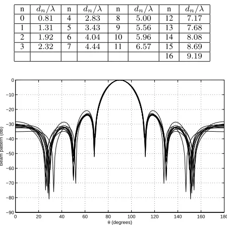
SENSORLOCATIONSFORTHEBROADSIDEDESIGNEXAMPLE WITH COMBINED MINIMISATION.

n dn/λ n dn/λ n dn/λ n dn/λ

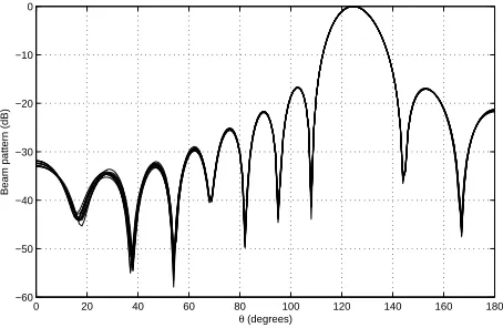
0 0_.81 ₄ 2_.83 ₈ 5_.00 ₁₂ 7_.17 1 1_.31 ₅ 3_.43 ₉ 5_.56 ₁₃ 7_.68 2 1_.92 ₆ 4_.04 ₁₀ 5_.96 ₁₄ 8_.08 3 2_.32 ₇ 4_.44 ₁₁ 6_.57 ₁₅ 8_.69 16 9_.19

0 20 40 60 80 100 120 140 160 180

−90 −80 −70 −60 −50 −40 −30 −20 −10 0

θ (degrees)

Beam pattern (dB)

Fig. 6. Responses for the broadside example with two-step minimisation.

between responses at different normalised frequencies. It is likely that this decrease in performance is due to the fact that there is no redesign of the weight coefficients after the merger of sensors on directly adjacent grid locations. The effect of discarding small non-zero valued coefficients is negligible compared to this. As a result, reducing the threshold below which coefficients are discarded will only offer a small improvement, while in some cases drastically increasing the number of non-zero valued coefficients. If improving the final value of||LTw||2 is desirable, then the easiest way would be to put a tighter constraint on the value in the first place.

Figs. 6 and 7 show the response obtained by the two-step l1 minimisation and combined minimisation methods respectively. For completeness the locations for the combined minimisation are also shown in Tab. VIII.

In both cases the mainlobe is at the correct location ofθ=

0 20 40 60 80 100 120 140 160 180

−70 −60 −50 −40 −30 −20 −10 0

θ (degrees)

Beam pattern (dB)

Fig. 7. Responses for the broadside example with combined minimisation.

TABLE IX

OFF-BROADSIDEPERFORMANCECOMPARISON FORTDL SPARSITY. Method CLS Two-Step

Mean||w||0 per TDL 25 16.4

||pr−wHS||2 0.82 0.82

||LT_w||

2 0.031 0.075

90◦

and there is sufficient sidelobe attenuation. The effect of the increase in the value of||LTw||2for the combined method can clearly be seen here. The performance in terms of the FI is clearly not as good in the sidelobe regions as it is for the other method. This, coupled with the fact that the two-step method gives us an array with less sensors and less coefficients per sensor, allows us to conclude that the method with the two-step

l1 minimisation is the best of the two.

We could redesign the coefficients for the locations found using the combined minimisation in (33) with another l1 minimisation as with the first proposed method for TDL sparsity in (28). However, there appears to be no advantage in doing this over using the first method on its own, as the second method in (33) tends to result in more active sensor locations. This would also mean it was unnecessary to include the TDL sparsity in the minimisation in the first place in (33).

2) Off-Broadside Examples: Here we only compare the two-step method in (28) with the CLS redesigned example us-ing the locations obtained by (23), as it has already been shown in the broadside example that the combined minimisation method has no real advantages. Tab. IX summarises the design results of the two methods. Note that the aperture length, number of active locations and mean adjacent separation are not shown, as both have used the same sensor locations.

Here we can see that redesigning the coefficients using an l1 minimisation has successfully reduced the number of coefficients per sensor location. However, this reduction in the number of coefficients has come at the cost of increasing the final value of ||LTw||2. As a result, we would expect more variation in the response at different normalised frequencies. However, there has been no change in the value of ||p_r−

wHS||2, suggesting the response at the reference frequency is still as close to the desired response as it previously was. The same criterion for removing small coefficients was applied to both design examples – any TDL coefficient with a value smaller than1×10−6_{is discarded. As with the broadside case,} this did not change the total number of coefficients that were present for the CLS design example.

D. Robust Sparse Array Design Example

We now consider a broadside design example in order to verify the effectiveness of the method for designing an FIB with robustness against a norm-bounded steering vector error. Here the same parameters as used for the previous broadside design examples are considered. In addition, the values ofε= 5 andγ= 0.0001are also used when solving (42).

When deciding if a response is robust or not we randonly generateN = 1000error vectors that meet the norm-bounded constraint in (41). For the nth _{error vector the achieved}

TABLE X

SENSORLOCATIONSFORTHEROBUSTSPARSEARRAYDESIGN

EXAMPLE.

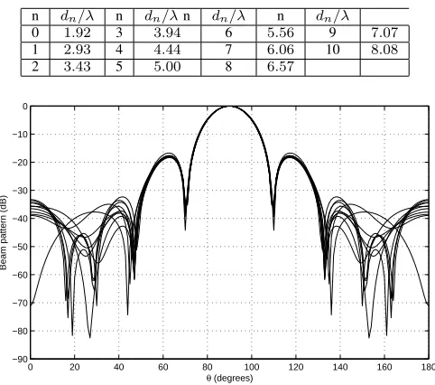
n dn/λ n dn/λn dn/λ n dn/λ

0 1_.92 ₃ 3_.94 ₆ 5_.56 ₉ 7_.07 1 2_.93 ₄ 4_.44 ₇ 6_.06 ₁₀ 8_.08 2 3_.43 ₅ 5_.00 ₈ 6_.57

0 20 40 60 80 100 120 140 160 180

−90 −80 −70 −60 −50 −40 −30 −20 −10 0

θ (degrees)

Beam pattern (dB)

Fig. 8. Designed response without temporal sparsity.

is found and the average achieved response is given by

¯

p(Ωk, θl) =

1 N

N−1

∑

n=0

pn(Ωk, θl), (50)

which is then used to find the normalised variance of the achieved array response,

var(Ωk, θl) = 1

N

N−1

∑

n=0

|pn(Ωk, θl)−p¯(Ωk, θl)|2

|p¯(Ωk, θl)|

, (51)

A close match between mean achieved and designed re-sponses, along with low normalised variance levels, would indicate that robustness has been achieved.

After discarding negligible locations and merging those on directly adjacent grids we end up with the 11 active sensor locations detailed in Tab. X, giving a mean adjacent sensor separation of0.62λ. However, this process will again mean the weight coefficients may no longer be optimal for the location we have. The coefficients were however used to find the values

σ= 0.035562and γ= 0.23732 that were used solving (49). The result was a set of weight coefficients without zero values (i.e. as expected no TDL sparsity).

Fig. 8 shows the resulting designed response for each of the sampled frequencies. We can see that for each frequency the mainlobe is in the desired location, and sufficient sidelobe attenuation and a good (especially around the mainlobe) FI property is achieved. Fig. 9 shows the mean achieved response, which is a close match to the designed one. Along with the low normalised variance levels shown in Fig. 10, this indicates a robust response has been achieved.

The next one is for designing a temporally sparse robust FIB. With the coefficients obtained in the first step, the values of α= 0.87448, σ= 0.035562 andγ= 0.23732 were found for use in solving (43). However, using these constraint values

0 20 40 60 80 100 120 140 160 180

−50 −45 −40 −35 −30 −25 −20 −15 −10 −5 0

θ (degrees)

Beam pattern (dB)

Fig. 9. Mean achieved response without temporal sparsity.

0 20 40 60 80 100 120 140 160 180

0 0.05 0.1 0.15 0.2 0.25 0.3 0.35

θ (degrees)

Normalised variance of beam pattern

Fig. 10. Normalised variance levels without temporal sparsity.

failed to give a temporally sparse solution. As a result the value of α was increased to 0.9 and a solution showing temporal sparsity was achieved. On average there was a reduction of

13.1 non-zero valued coefficients per TDL.

The designed response, mean achieved response and nor-malised variance levels are shown in Figs. 11, 12 and 13

0 20 40 60 80 100 120 140 160 180

−90 −80 −70 −60 −50 −40 −30 −20 −10 0

θ (degrees)

Beam pattern (dB)

0 20 40 60 80 100 120 140 160 180 −45

−40 −35 −30 −25 −20 −15 −10 −5 0

θ (degrees)

Beam pattern (dB)

Fig. 12. Mean achieved response with temporal sparsity.

0 20 40 60 80 100 120 140 160 180

0 0.02 0.04 0.06 0.08 0.1 0.12 0.14 0.16 0.18

θ (degrees)

Normalised variance of beam pattern

Fig. 13. Normalised variance levels with temporal sparsity.

respectively. Again an acceptable designed response has been achieved, with satisfactory mean achieved response and nor-malised variance level.

VI. CONCLUSIONS

In this paper, a series of CS-based methods for the de-sign of sparse arrays for wideband beamforming including frequency invariant beamforming has been proposed. Two levels of sparsity were considered: one is the sparsity in sensor locations and the other one is the sparsity of the TDL coefficients associated with each sensor in order to reduce the implementation complexity of each TDL.

Although CS-based methods have been proposed for the design of narrowband sparse arrays, their extension to the wideband case is not straightforward, as there are multiple coefficients along a TDL associated with each sensor and it is not sufficient to simply minimize the l1 norm of the weight vector. Instead all the coefficients along a TDL have to be simultaneously minimized, which was achieved by a modified l1 norm minimization method. An extra constraint based on the concept of response variation was then added to ensure a frequency invariant response. To further improve the sparsity of array locations, an iterative process is employed with a reweighting term introduced in the cost function so

that locations with small contributions are penalised in the next iteration, while locations with a large contribution are replicated.

For the design of sparse TDLs, two methods were proposed. The first one is based on a two-step l1 minimisation, where we first obtain the sparse sensor locations using the above proposed methods and then find the minimum number of non-zero valued coefficients for the fixed set of sensor locations. In the second method, we consider the sparsity in sensor locations and TDL coefficients simultaneously. It seems that the second one may give a better result. However, based on our design results, the first one has achieved a better result. Details of a further constraint, which can ensure the solution is robust against steering vector errors were also given. This constraint works by keeping the maximum change in array response, due to a norm-bounded steering vector error, below a predetermined acceptable level.

Various design examples have been presented, with com-parisons also drawn with a GA-based method. Similar perfor-mance levels are achieved but the GA design takes consider-ably longer to reach the solution, highlighting the advantage of our proposed design methods.

REFERENCES

[1] M. S. Brandstein and D. Ward, Eds., Microphone Arrays: Signal Processing Techniques and Applications. Berlin: Springer, 2001. [2] W. Liu and S. Weiss,Wideband Beamforming: Concepts and Techniqeus.

Chichester, UK: John Wiley & Sons, 2010.

[3] S. C. Chan and H. H. Chen, “Uniform concentric circular arrays with frequency-invariant characteristics–theory, design, adaptive beamform-ing and DOA estimation,” IEEE Transactions on Signal Processing, vol. 55, pp. 165–177, January 2007.

[4] H. W. Chen and W. Ser, “Design of robust broadband beamformers with passband shaping characteristics using Tikhonov regularization,”IEEE Transactions on Audio, Speech, and Language Processing, vol. 17, no. 4, pp. 665–681, May 2009.

[5] M. Crocco and A. Trucco, “A computationally efficient procedure for the design of robust broadband beamformers,”IEEE Transactions on Signal Processing, vol. 58, no. 10, pp. 5420–5424, October 2010. [6] ——, “Design of robust superdirective arrays with a tunable tradeoff

between directivity and frequency-invariance,” IEEE Transactions on Signal Processing, vol. 59, no. 5, pp. 2169–2181, May 2011. [7] P. Jarske, T. Saramaki, S. K. Mitra, and Y. Neuvo, “On properties and

design of nonuniformly spaced linear arrays,” IEEE Transactions on Acoustics, Speech, and Signal Processing, vol. 36, no. 3, pp. 372 –380, March 1988.

[8] R. L. Haupt, “Thinned arrays using genetic algorithms,”IEEE Transac-tions on Antennas and Propagation, vol. 42, no. 7, pp. 993–999, July 1994.

[9] K.-K. Yan and Y. Lu, “Sidelobe reduction in array-pattern synthesis using genetic algorithm,” IEEE Transactions on Antennas and Propa-gation, vol. 45, no. 7, pp. 1117–1122, July 1997.

[10] K. Chen, Z. He, and C. Han, “Design of 2-dimensional sparse arrays using an improved genetic algorithm,” in Proc. IEEE Workshop on Sensor Array and Multichannel Processing, July 2006, pp. 209–213. [11] L. Cen, W. Ser, Z. L. Yu, and S. Rahardja, “An improved genetic

algorithm for aperiodic array synthesis,” in Proc. IEEE International Conference on Acoustics, Speech, and Signal Processing, April 2008, pp. 2465 –2468.

[12] M. B. Hawes and W. Liu, “Location optimisation of robust sparse antenna arrays with physical size constraint,” IEEE Antennas and Wireless Propagation Letters, pp. 1303–1306, November 2012. [13] Z. Li, K. F. C. Yiu, and Z. Feng, “A hybrid descent method with

genetic algorithm for microphone array placement design,”Applied Soft Computing, vol. 13, no. 3, pp. 1486–1490, 2013.

[15] M. R. Bai, J.-H. Lin, and K.-L. Liu, “Optimized microphone deployment for near-field acoustic holography: to be, or not to be random, that is the question,” Journal of Sound and Vibration, vol. 329, no. 14, pp. 2809–2824, 2010.

[16] M. Crocco and A. Trucco, “Stochastic and analytic optimization of sparse aperiodic arrays and broadband beamformers with robust superdi-rective patterns,”IEEE Transactions on Audio, Speech, and Language Processing, vol. 20, no. 9, pp. 2433–2447, Nov 2012.

[17] E. Candes, J. Romberg, and T. Tao, “Robust uncertainty principles: exact signal reconstruction from highly incomplete frequency information,”

IEEE Transactions on Information Theory, vol. 52, no. 2, pp. 489– 509, February 2006.

[18] L. Li, W. Zhang, and F. Li, “The design of sparse antenna array,”CoRR, vol. arXiv.org/abs/0811.0705, 2008.

[19] G. Prisco and M. D’Urso, “Exploiting compressive sensing theory in the design of sparse arrays,” inProc. IEEE Radar Conference, May 2011, pp. 865 –867.

[20] L. Carin, “On the relationship between compressive sensing and random sensor arrays,” IEEE Antennas and Propagation Magazine, vol. 51, no. 5, pp. 72 –81, October 2009.

[21] G. Oliveri and A. Massa, “Bayesian compressive sampling for pattern synthesis with maximally sparse non-uniform linear arrays,” IEEE Transactions on Antennas and Propagation, vol. 59, no. 2, pp. 467– 481, 2011.

[22] G. Oliveri, M. Carlin, and A. Massa, “Complex-weight sparse linear array synthesis by bayesian compressive sampling,”IEEE Transactions on Antennas and Propagation, vol. 60, no. 5, pp. 2309–2326, 2012. [23] M. B. Hawes and W. Liu, “Robust sparse antenna array design via

compressive sensing,” in Proc. International Conference on Digital Signal Processing, 2013.

[24] ——, “Compressive sensing based approach to the design of lin-ear robust sparse antenna arrays with physical size constraint,”

IET Microwaves, Antennas & Propagation, 2014, DOI: 10.1049/iet-map.2013.0469.

[25] ——, “A quaternion-valued reweighted minimisation approach to sparse vector sensor array design,” inProc. of the International Conference on Digital Signal Processing, Hong Kong, August 2014.

[26] E. Candes, M. Wakin, and S. Boyd, “Enhancing sparsity by reweighted

l1minimization,”Journal of Fourier Analysis and Applications, vol. 14,

pp. 877–905, 2008.

[27] B. Fuchs, “Synthesis of sparse arrays with focused or shaped beam-pattern via sequential convex optimizations,” IEEE Transactions on Antennas and Propagation, vol. 60, no. 7, pp. 3499 –3503, July 2012. [28] G. Prisco and M. D’Urso, “Maximally sparse arrays via sequential

con-vex optimizations,”IEEE Antennas and Wireless Propagation Letters, vol. 11, pp. 192 –195, 2012.

[29] S. Winter, H. Sawada, and S. Makino, “On real and complex valuedl1

-norm minimization for overcomplete blind source separation,” inProc. of IEEE Workshop on Applications of Signal Processing to Audio and Acoustics, October 2005, pp. 86 – 89.

[30] M. B. Hawes and W. Liu, “Sparse microphone array design for wideband beamforming,” in Proc. International Conference on Digital Signal Processing, 2013.

[31] W. Liu, S. Weiss, J. G. McWhirter, and I. K. Proudler, “Frequency in-variant beamforming for two-dimensional and three-dimensional arrays,”

Signal Processing, vol. 87, pp. 2535–2543, November 2007.

[32] W. Liu and S. Weiss, “Design of frequency invariant beamformers for broadband arrays,”IEEE Transactions on Signal Processing, vol. 56, no. 2, pp. 855–860, February 2008.

[33] H. Duan, B. P. Ng, C. M. See, and J. Fang, “Applications of the SRV constraint in broadband pattern synthesis,”Signal Processing, vol. 88, pp. 1035–1045, April 2008.

[34] Y. Zhao, W. Liu, and R. J. Langley, “An application of the least squares approach to fixed beamformer design with frequency invariant constraints,”IET Signal Processing, vol. 5, pp. 281–291, June 2011. [35] ——, “Adaptive wideband beamforming with frequency invariance

constraints,”IEEE Transactions on Antennas and Propagation, vol. 59, no. 4, pp. 1175–1184, April 2011.

[36] H.-J. Kang and I.-C. Park, “Fir filter synthesis algorithms for minimizing the delay and the number of adders,”IEEE Transactions on Circuits and Systems II: Analog and Digital Signal Processing, vol. 48, no. 8, pp. 770–777, 2001.

[37] D. Maskell, “Design of efficient multiplierless fir filters,”IET, Circuits, Devices Systems, vol. 1, no. 2, pp. 175–180, 2007.

[38] R. Mahesh and A. Vinod, “Low complexity flexible filter banks for uni-form and non-uniuni-form channelisation in software radios using coefficient

decimation,”IET Circuits, Devices Systems, vol. 5, no. 3, pp. 232–242, 2011.

[39] E. Mabande, A. Schad, and W. Kellermann, “Design of robust superdi-rective beamformers as a convex optimization problem,” inProc. IEEE International Conference on Acoustics, Speech, and Signal Processing, April 2009, pp. 77–80.

[40] R. Nongpiur and D. Shpak, “L -infinity norm design of linear-phase robust broadband beamformers using constrained optimization,” IEEE Transactions on Signal Processing, vol. 61, no. 23, pp. 6034–6046, Dec 2013.

[41] H. Chen, W. Ser, and J. Zhou, “Robust nearfield wideband beamformer design using worst case mean performance optimization with passband response variance constraint,”IEEE Transactions on Audio, Speech, and Language Processing, vol. 20, no. 5, pp. 1565–1572, July 2012. [42] Y. Zhao and W. Liu, “Robust fixed frequency invariant beamformer

design subject to norm-bounded errors,”IEEE Signal Processing Letters, vol. 20, pp. 169–172, February 2013.

[43] C. Research, “CVX: Matlab software for disciplined convex program-ming, version 2.0 beta,” http://cvxr.com/cvx, September 2012. [44] M. Grant and S. Boyd, “Graph implementations for nonsmooth convex

programs,” inRecent Advances in Learning and Control, ser. Lecture Notes in Control and Information Sciences, V. Blondel, S. Boyd, and H. Kimura, Eds. Springer-Verlag Limited, 2008, pp. 95–110, http://stanford.edu/ boyd/graph dcp.html.

Matthew Hawes was born on The Wirral, United Kingdom, in September 1987. He received his M.Eng degree in Electronic and Communications Engineering from The University of Sheffield in 2010. Since then he has been working towards his Ph.D in the communications research group at the same university. His research interests include sparsity in array signal processing and compressive sensing.