promoting access to White Rose research papers
White Rose Research Online
[email protected]
Universities of Leeds, Sheffield and York
http://eprints.whiterose.ac.uk/
This is the published version of an article in
Physical Review A - Atomic,
Molecular, and Optical Physics
White Rose Research Online URL for this paper:
http://eprints.whiterose.ac.uk/id/eprint/78435
Published article:
Freeman, JR, Maysonnave, J, Khanna, S, Linfield, EH, Davies, AG, Dhillon, SS
and Tignon, J (2013)
Laser-seeding dynamics with few-cycle pulses:
Maxwell-Bloch finite-difference time-domain simulations of terahertz quantum cascade
lasers.
Physical Review A - Atomic, Molecular, and Optical Physics, 87 (6).
063817. ISSN 1050-2947
Laser-seeding dynamics with few-cycle pulses: Maxwell-Bloch finite-difference time-domain
simulations of terahertz quantum cascade lasers
Joshua R. Freeman,1,*Jean Maysonnave,1Suraj Khanna,2Edmund H. Linfield,2A. Giles Davies,2 Sukhdeep S. Dhillon,1and J´erˆome Tignon1
1Laboratoire Pierre Aigrain, Ecole Normale Sup´erieure, CNRS (UMR 8551), Universit´e Pierre et Marie Curie,
Universit´e D. Diderot, 75231 Paris Cedex 05, France
2School of Electronic and Electrical Engineering, University of Leeds, Woodhouse Lane, Leeds LS9 2JT, United Kingdom
(Received 8 March 2013; published 12 June 2013)
We implement a Maxwell-Bloch simulation for a two-level system within the finite-difference time-domain method to simulate the seeding of lasers by broadband pulse injection. The model does not make the slowly varying envelope approximation, and the full electromagnetic field is simulated so that we are able to obtain time-resolved seeding by few-cycle pulses. The model is compared to recent results on seeding of THz quantum cascade lasers to aid in the interpretation of their complex signals. The simulations are found to be in good agreement with the data when gain recovery times of 15 ps are used. Furthermore, we find that the emission from the laser depends only weakly on the seed used to initiate laser action. The model is readily applicable to any seeded laser system where few-cycle seed pulses are used.
DOI:10.1103/PhysRevA.87.063817 PACS number(s): 42.55.Px
I. INTRODUCTION
Optical injection seeding is widely used to imprint some desirable characteristic of one “seed” laser onto another laser. The desirable characteristic is most often frequency stability; by using a seed laser with a stable frequency, it is possible to reduce the mode partition noise in modulated diode lasers [1] and produce narrowband pulses fromQ-switched pulsed lasers [2,3].
The use of laser seeding, however, is not limited to frequency stabilization. We have recently made use of optical injection seeding to stabilize the phase of a laser [4]. The sta-bilized laser was a quantum cascade laser (QCL) operating in the terahertz (THz) region of the electromagnetic spectrum [5] and the seed was a broadband single-cycle pulse generated by a biased photoconductive antenna illuminated by a mode-locked Ti:sapphire laser. In doing this, we are making use of the fact that the pulse length of the femtosecond pulse, less than 100 fs, is significantly shorter than the period of the terahertz radiation produced by the QCL. Each femtosecond pulse is split, with one portion used to generate a single-cycle THz pulse by the use of a photoconductive antenna. The single-cycle pulse is then injected into the QCL cavity at the same moment that the QCL is brought above threshold. In this way, the THz QCL emission is initiated by the single-cycle THz pulse rather than the spontaneous emission. By seeding the laser emission in this way, the phase of the QCL emission is dictated by the fem-tosecond pulse. Thus, we are making use of the well-defined temporal aspect of the femtosecond seed pulse rather than conventional seeding, where it is the well-definedfrequency aspect that is used. With the phase of the QCL emission stabilized to the femtosecond pulse, we are able to use the other portion of the split femtosecond pulse to sample coherently the THz field in an electro-optic crystal. It is interesting to note that while optical injection has not been used to stabilize the frequency emission of a QCL, an electrical feedback
*[email protected]; [email protected]
technique has been used to stabilize the QCL emission frequency [6].
The prospect of coherent detection of laser radiation could find technological applications because both time-domain and spectral information are available in the same measurement. In addition, this radiation falls in the traditionally underexploited THz region of the electromagnetic spectrum [7]. Besides the technological interest of this measurement, it also provides a means to study laser emission in unprecedented detail and gain insight into the operation of QCLs. The type of signals observed from seeded QCLs can vary significantly from qua-siconstant [4] to a single pulse per round trip [8] and multiple pulses per round trip [9]. This variety and complexity of signals hints at the dynamics of QCLs. The important lifetimes for QCLs, namely the gain recovery time,T1, the dephasing time,
T2, and the photon lifetime,Tph, are all of the order of 1–50 ps
and the cavity round-trip time is typically the same as or longer than these times, leading to complex dynamics [10].
The ultrafast dynamics of QCLs has become of particular interest recently due to progress in mode-locking of QCLs both in the mid-IR [11] and THz [12,13] regions of the spectrum. The role of the laser dynamics, particularly the gain recovery time, T1, is a critical parameter for stable mode-locking and should also strongly affect the temporal output of seeded QCLs. Despite the importance of this parameter, there has been only one attempt to measure this parameter in THz QCLs directly [14] due to the difficulty of the measurement.
To gain a deeper understanding of the processes involved in this type of seeding by single-cycle pulses and to understand the complex signals observed, we have carried out numerical time-domain simulations using the Maxwell-Bloch formalism. These simulations help explain the role and the effect of the gain recovery time on the coherent field we observe. In addition, we are able to assess how changing the optical seed affects the emission from the laser.
II. MODEL
JOSHUA R. FREEMANet al. PHYSICAL REVIEW A87, 063817 (2013)
equations within the slowly varying envelope approximation. These methods have successfully described the dynamics of QCLs and have been used to model coherent instabilities [15], self-induced transparency mode-locking [16], and most recently, active mode-locking [17]. For the present work, we again make use of the Maxwell-Bloch equations. However, rather than make the slowly varying envelope approximation, we follow the method of Ziolkowski et al. [18] to solve the equations using the finite-difference time-domain (FDTD) method. In doing so, we directly compute the electric field rather than the envelope of the field. This is particularly important in our case because the seed pulse is single-cycle and therefore cannot be approximated by a slowly varying envelope. A similar method was used by Darmoet al.[19] to understand the interaction of a THz pulse with a two-level gain medium, but the laser dynamics was not investigated.
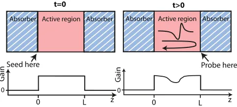
The system being investigated is ideal to simulate because the experiment and simulation are conceptually identical. In the experiment, the sample is prepared in a nonequilibrium state before the seed pulse arrives, ensuring that there is no laser emission in the cavity before the seed pulse arrives and any emission is initiated by the seed pulse. The output from the sample can then be measured coherently as a function of time for the first few nanoseconds of the emission. The simulation is done in the same way: att=0, a seed pulse is injected into the cavity, containing a population inversion, and the output is monitored over time, as shown schematically in Fig.1.
We follow the formulation of Ref. [17] and describe the QCL gain region as an open two-level system with an upper level (2) and a lower level (1), with the latter always empty. For that case, the Bloch equations are
∂tρ12 = −
1
T2 −
j ω12
ρ12+ExM j¯h w−
2ExX
jh¯ ρ12, (1)
∂tw= 2ExM
j¯h (ρ ∗
12−ρ12)−
w−w0
T1
. (2)
Here,ρ1andρ2are the fractional populations of states 1 and
2,ρ12=ρ21∗ represents the coherence between the two states,
andw=ρ2−ρ1is the population inversion between the two
states. The energy of the transition between the two levels is
t=0 L G ain 0 Probe here 0 t>0 Seed here L 0 0 G ain z z Active region Absorber Absorber Active region Absorber Absorber
FIG. 1. (Color online) Schematic of the simulation. The active region has a relative permittivity ofr =12.9, a waveguide loss of 3 cm−1, and an unsaturated gain of 21 cm−1. The absorber regions have a relative permittivity ofr =1, a loss of 3×104 cm−1, and zero gain. The seed is launched at t=0 on the left facet and the signal is probed just outside the right facet.
¯
hω12,M=e2|x|1 is the dipole matrix element, andEx is the electric field coupling to the transition. The value of the population inversion without the presence of radiation isw0
and the characteristic lifetime for the return to this value isT1,
the gain recovery time. The dephasing time for the transition is given byT2. We have also included a term in Eq.(1)that is
usually ignored:
X= e
2(2|x|2 − 1|x|1). (3) For atomic systems this term will clearly be zero as the wave functions of the two states are centered around the same point in space. However, for our case of intersubband transitions in a superlattice under an applied bias, the value ofX will be nonzero. We have performed simulations with realistic values of this parameter (X=16 nm for the active region under investigation) and found that the effect on the resulting signal is very small. Therefore, for the remainder of this work we shall ignore this term. It should be noted, however, that for some active regions with highly diagonal transitions (e.g., [20]) this factor may become important. Another point to note is that rather than follow Ref. [17] and parametrize the last term of Eq.(2)with a pumping parameter,J ∝λ= w0
T1, proportional to the injection current, we prefer to use the unclamped population inversion as we have a reliable measurement of the unclamped gain in our devices [21].
To obtain real equations for computation and agreement with the notation of Ziolkowskiet al.[18], we make the substi-tution 2ρ12 =ρa−jρband, by recalling that the polarization of the medium isPx= −2N Mρa(Nis the number of identical two-level systems), we link the Maxwell and Bloch equations to obtain the set of real equations:
∂tHy = − 1
μ0
∂Ex
∂z , (4)
∂tEx = − 1 ε ∂Hy ∂z − N M εT2
ρa+
N Mω21
ε ρb−lEx, (5)
∂tρa = − 1
T2ρa+ω12ρb, (6)
∂tρb = − 1
T2ρb−ω12ρa+
2ExM ¯
h w, (7)
∂tw= −
w−w0
T1
−2ExM ¯
h ρb. (8)
Here we have also added at term, (−lEx), to account for the waveguide loss. This set of equations is then solved using the FDTD predictor-corrector method proposed by Ref. [18]. We do not analytically factor out the decay termsT1 andT2
because this is only possible for a single-pass model [18]; we do not find that this introduces problems of numerical stability.
III. SAMPLE
Equations(4)–(8) will propagate an electromagnetic field traveling in thezdirection through a homogeneous medium containing N two-level systems per unit volume [22]. The Fabry-P´erot cavity of the active region is formed by imposing a refractive index ofr =1 outside the active region, indicated in Fig.1. This leads to a reflection of around 30% at the bound-ary, in good agreement with other studies and experiments [23–25]. The region outside the cavity is made highly lossy to
[image:3.608.52.294.571.681.2]TABLE I. Parameters used in the simulations.
Symbol Name Value(s)
εr Background relative permittivity 12.9 T1 Gain recovery time 5–50 ps T2 Dephasing time 2.35 ps w0 Equilibrium population inversion 1 N Number of oscillators 3.7×10²⁰m−3 M/e Dipole matrix element 6.2 nm ω12 Transition frequency 2π×2.45 THz
l Waveguide loss 3 cm−1
L Cavity length 1.5 and 3 mm
ensure that reflections from the fixed boundary conditions are suppressed.
The seed pulse is launched into the cavity by modulating the value of the electric field on the left facet. However, the field value on this facet must be allowed to vary freely before the seed returns. This places an upper bound on the duration of the seed pulse, which is the cavity round-trip time. In our case, the seed easily fulfills this criterion. We approximate the seed pulse generated by the photoconductive antenna as a single cycle pulse with a characteristic width of 0.35 ps, which we measure experimentally. We also observe an echo in the seed pulse experimentally, around 36 ps after the main pulse, due to the finite thickness of the photoconductive antenna, and we have included this effect in the seed.
The active region that we have chosen to simulate is a bound-to-continuum design [26], with the active region modified to emit at 2.45 THz. The active region was selected because it was also used in Ref. [21], where the maximum unclamped gain was measured to be 21 cm−1. We have
used this value to choose the value ofN, shown in Table I, together with the other parameters required by the numerical simulation. The values of ω12 andT2 were found from the
center frequency and bandwidth of the laser spectra, and the value ofw0was chosen to be 1 for the peak value of the gain. The value ofMwas calculated from the band structure of the active region.
The loss for the waveguide was found by comparing the value of the clamped gain from measurements when the laser is operating and the gain clamped [25]. We find a waveguide loss ofαw=3 cm−1 after accounting for the mirror losses. Therefore, the only parameter that is not well known isT1, the
gain recovery time. In the following simulations, we use values ofT1between 5 and 50 ps and we study the dependence of the
simulation on this value. A space step size ofdz=λ/150 and a time step ofdt=dz/c0were used for the FDTD simulations. For the cavity length,L, we will compare two commonly used cavity lengths: 1.5 and 3 mm. The cavity length is an easy parameter to change experimentally and can provide insight into the laser dynamics because it changes the ratio between the cavity round-trip time and the gain recovery time. The cavity round-trip times for 1.5 and 3 mm cavities are 36 and 72 ps, respectively. Changing the cavity length also changes the photon lifetime in the cavity, estimated to be 11 and 17 ps, respectively, for the 1.5 and 3 mm cavity. In terms of loss, the total loss will be 11 and 7 cm−1, respectively, for the 1.5 and
3 mm cavity. Also, given the smaller free spectral range of the
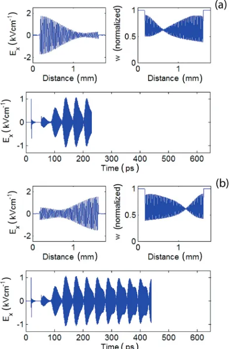
FIG. 2. (Color online) Stills from a video of a simulation for a 1.5 mm cavity using a gain recovery time of 20 ps, showing the simulation after (a) 230 ps and (b) 440 ps. The video is available in the Supplemental Material.
longer Fabry-P´erot cavity, there will be more modes present in the longer cavity.
It is interesting to compare the value ofN found above to the number of carriers present in the sample through doping. The average nominal doping in the active region is 0.37× 10²² m−3. By taking into account the number of periods (90)
and the overlap of the optical mode with the active region (∼30%), we find a maximum possible number of active carriers of 7.8×10²² m−3. Comparing this with the value of
N in TableIimplies a conversion efficiency of 0.5%, in good agreement with the 0.5–5 % commonly measured for this type of design by more conventional methods [27,28].
IV. RESULTS
Figure2shows the results from a typical simulation with
[image:4.608.48.295.82.211.2]JOSHUA R. FREEMANet al. PHYSICAL REVIEW A87, 063817 (2013)
0 200 400 600
-1 0 1 2 3 4 5
0 200 400 600
-1 0 1 2 3 4 5
Time (ps)
L = 3mm
(b)
5ps 20ps
E
lec
tr
ic
field
(nor
m
a
liz
e
d)
Time (ps)
50ps (a)
L = 1.5mm
FIG. 3. (Color online) Numerical simulations for (a) 1.5 mm and (b) 3 mm cavities using gain recovery times ofT1=5, 20, and 50 ps. The simulations are normalized and offset for clarity.
electron diffusion counteracts the effect of SHB. However, this effect is thought to be weak in QCLs [15,17] and the model assumes that there is no lateral electron diffusion.
It is also interesting to note that the node in the SHB of the population inversion does not occur at the same position as the minimum of the intracavity electric field. This is because the electric field, Ex, and the population inversion, w, are connected through the polarization, causing the population inversion to lag the electric field.
From the simulation we record the emission from the laser cavity at the opposite facet to the injection (as in the experimental measurements) and we plot the electric field emission from the laser cavity over time. We show this in Fig.3for 1.5 and 3 mm cavities andT1=5, 20, and 50 ps.
The differences between the two cavity lengths are quite marked. The simulated signals from the shorter, 1.5 mm cavity
shows essentially one pulse for each cavity round trip, while the longer 3 mm cavity shows signals that are more complex, with two or three pulses distinguishable for each cavity round trip. One reason for more complex pulse formation is the larger number of modes operating above threshold, leading to more intermode beating. As the gain recovery time,T1, is decreased
from 50 to 5 ps, it is noticeable how the emission intensity tends to become more continuous. This is because the faster gain recovery allows amplification even a short time after a pulse has passed.
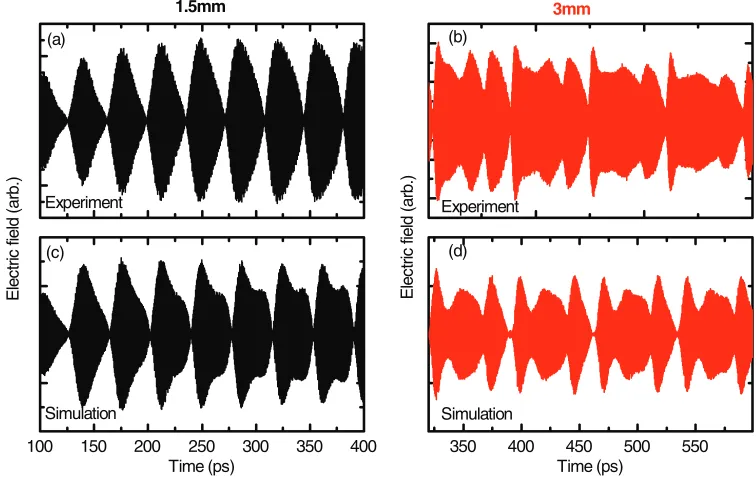
We can now make a closer comparison between these simulations and the data that we typically measure for this active region, shown in Fig.4. The data have been acquired from two samples with lengths of 1.5 and 3 mm. The experimental setup is the same as that in Refs. [4] and [9], and the details can be found in those articles.
The simulations that give the best agreement with the data use a gain recovery time of 15 ps, and these are also shown in Fig. 4 for comparison. We see that there is good qualitative agreement between the simulations and experiment for both cavity lengths under investigation, particularly given the variety of seeded signals that can be generated. For the 1.5 mm cavity, the numerical simulation reproduces several features of the data, including one pulse per round trip and an asymmetric pulse shape. The asymmetric pulse shape appears to originate from the amplification of the seed pulse on the first pass in the cavity. For the 3 mm cavity, the emission is much more complex, however the essential features of the data are captured in the simulation; both show three identifiable pulses per round trip and a null in the field in each round trip.
The value of 15 ps for the gain recovery time is less than that found by Greenet al.[14] of 50 ps for a similar THz QCL design, but larger than the values measured for mid-IR QCLs of 2–3 ps [29]. Another relevant work by Scalariet al.[30] found
100 150 200 250 300 350 400 350 400 450 500 550 (d)
(c)
(b)
E
lec
tr
ic
field
(ar
b.
)
Time (ps)
1.5mm 3mm
E
lec
tr
ic
field
(ar
b.
)
(a)
Experiment
Simulation Simulation
Time (ps) Experiment
FIG. 4. (Color online) A comparison between experimental data and simulation for 1.5 and 3 mm cavities. Parts (a) and (b) show experimental data for 1.5 and 3 mm cavities, respectively. Parts (c) and (d) show the corresponding simulations. The value of gain recovery time used in these simulations is 15 ps.
[image:5.608.53.290.71.219.2] [image:5.608.114.492.476.715.2]0 100 200 300 400 500 800 900 1000 (b)
Time (ps) (a)
E
lec
tr
ic
field
(ar
b.
unit
s)
E
lec
tr
ic
field
(ar
b.
unit
s)
Time (ps)
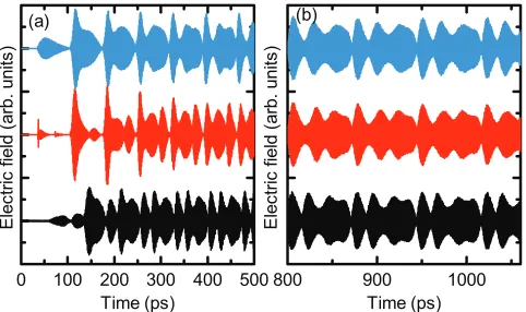
FIG. 5. (Color online) A comparison of different seed pulses for a 3 mm cavity. Blue (upper): The cavity is seeded by a narrow-band pulse resonant with the laser transition and is 50 ps long. Red (middle): A short seed pulse, as in Fig.4. Black (lower): A random perturbation is made to the cavity and evolves. (a) The first 500 ps after the seed arrives. (b) Simulation after 1 ns. In this figure, the time delay of each trace has been shifted to facilitate comparison.
an upper state lifetime for a THz QCL of 12 ps [31], much closer to the value we deduce here. The measurement of Green et al. might best be described as the system recovery time because the quantity measured in the pump-probe experiment was the photocurrent through the entire structure. Thus it may overestimate the microscopic gain recovery time that we use in our model.
We can also use this simulation to understand the de-pendence of the laser output on the seed pulse by changing the type of optical seed that we inject; Fig. 5 shows the results of these comparisons. We investigated two cases in addition to the experimental situation of an ultrashort pulse with a broad spectrum: (i) A narrowband pulse at the QCL frequency (Fig.5, blue) and (ii) random noise (Fig.5, black). The narrowband pulse, with a frequency of 2.45 THz and a duration of 50 ps, was chosen as a contrast to the single cycle seed pulse. The random seed represents an approximation of how the laser would start naturally (on spontaneous emission), a regime that we are unable to access experimentally due to the synchronization requirements of the measurement [9]. The random seed was approximated by introducing a random electric field perturbation along the entire length of the cavity att =0 and letting the emission evolve freely.
For each of these different seeds, we find that the resulting emission is remarkably similar after a few cavity round trips
(∼1 ns); see Fig. 5(b). This finding suggests that the exact form of the seed does not greatly affect the emission produced by the laser, and therefore the electric field that we measure experimentally from the laser is very similar to the emission from a free-running laser.
We have also investigated the effect of changing the seed amplitude on the QCL emission. While we do not see any change in the form of the emission at longer times, we do find that the “buildup” time is longer for weaker seed pulses.
V. CONCLUSIONS
We have developed a numerical simulation to describe the seeding of a laser by few-cycle broadband pulses by using a model based on Maxwell-Bloch equations solved under the FDTD framework. This model has been applied to the seeding of THz QCLs with single-cycle THz pulses and compared with the experimental results. The simulations are in good agreement with the experimental data, reproducing the differing signals observed for different cavity lengths. The least well known parameter in the model is the gain recovery time,
T1. However, we see good qualitative agreement with the data
when using a value of 15 ps, which compares favorably with the value previously found in Ref. [30]. This value, shorter than the round-trip time, suggests that commonly employed mode-locking techniques where the laser is continuously pumped will not be possible as the gain medium cannot store sufficient energy. However, synchronous pumping [32] techniques are possible routes to mode-locking [12,13].
The dependence of the electric field emission on the seed pulse was also examined. It was found that electric field emission from the QCL laser is largely insensitive to the type of seed used, implying that the experimentally observed signals closely resemble the “natural” emission of the QCL. This is somewhat counter to the more established idea of seeding that is conventionally used to fix the frequency of the laser to a seed laser.
ACKNOWLEDGMENTS
We are grateful for support from the “Agence Nationale de la Recherche” (ANR, Contract No. HI-TEQ ANR-09-NANO-017), the EPSRC (UK), the ERC programmes NOTES and TOSCA, and to the Royal Society and Wolfson Foundation. J.R.F. acknowledges funding from a Marie Curie fellowship (Grant No. 274602).
[1] K. Iwashita and K. Nakagawa,IEEE J. Quantum Electron.18, 1669 (1982).
[2] J. Yu, U. N. Singh, N. P. Barnes, and M. Petros,Opt. Lett.23, 780 (1998).
[3] S. Hannemann, E.-J. van Duijn, and W. Ubachs, Rev. Sci. Instrum.78, 103102 (2007).
[4] D. Oustinov, N. Jukam, R. Rungsawang, J. Madeo, S. Barbieri, P. Filloux, C. Sirtori, X. Marcadet, J. Tignon, and S. Dhillon, Nat. Commun. 1, 69 (2010).
[5] B. S. Williams,Nat. Photon.1, 517 (2007).
[6] S. Barbieri, P. Gellie, G. Santarelli, L. Ding, W. Maineult, C. Sirtori, R. Colombelli, H. Beere, and D. Ritchie,Nat. Photon.
4, 636 (2010).
[7] Y.-S. Lee, Principles of Terahertz Science and Technology (Springer, New York, 2009) .
[image:6.608.53.294.70.213.2]JOSHUA R. FREEMANet al. PHYSICAL REVIEW A87, 063817 (2013)
[9] J. Maysonnave, N. Jukam, M. S. M. Ibrahim, R. Rungsawang, K. Maussang, J. Mad´eo, P. Cavali´e, P. Dean, S. P. Khanna, D. P. Steenson, E. H. Linfield, A. G. Davies, S. S. Dhillon, and J. Tignon,Opt. Express20, 16662 (2012).
[10] G. H. van Tartwijk and G. P Agrawal,Prog. Quantum Electron.
22, 43 (1998).
[11] C. Y. Wang, L. Kuznetsova, V. M. Gkortsas, L. Diehl, F. X. Kartner, M. A. Belkin, A. Belyanin, X. Li, D. Ham, H. Schneider, P. Grant, C. Y. Song, S. Haffouz, Z. R. Wasilewski, H. Liu, and F. Capasso,Opt. Express17, 12929 (2009).
[12] S. Barbieri, M. Ravaro, P. Gellie, G. Santarelli, C. Manquest, C. Sirtori, S. P. Khanna, E. H. Linfield, and A. G. Davies,Nat. Photon.5, 306 (2011).
[13] J. R. Freeman, J. Maysonnave, N. Jukam, P. Cavalie, K. Maussang, H. E. Beere, D. A. Ritchie, J. Mangeney, S. S. Dhillon, and J. Tignon,Appl. Phys. Lett.101, 181115 (2012).
[14] R. P. Green, A. Tredicucci, N. Q. Vinh, B. Murdin, C. Pidgeon, H. E. Beere, and D. A. Ritchie, Phys. Rev. B 80, 075303 (2009).
[15] A. Gordon, C. Y. Wang, L. Diehl, F. X. K¨artner, A. Belyanin, D. Bour, S. Corzine, G. H¨ofler, H. C. Liu, H. Schneider, T. Maier, M. Troccoli, J. Faist, and F. Capasso, Phys. Rev. A
77, 053804 (2008).
[16] C. R. Menyuk and M. A. Talukder,Phys. Rev. Lett.102, 023903 (2009).
[17] V.-M. Gkortsas, C. Wang, L. Kuznetsova, L. Diehl, A. Gordon, C. Jirauschek, M. A. Belkin, A. Belyanin, F. Capasso, and F. X. K¨artner,Opt. Express18, 13616 (2010).
[18] R. W. Ziolkowski, J. M. Arnold, and D. M. Gogny,Phys. Rev. A52, 3082 (1995).
[19] J. Darmo, J. Kroll, and K. Unterrainer, inTheoretical Aspects of Time-domain Spectroscopy of Semiconductor Terahertz Gain Medium, AIP Conf. Proc. No. 893 (AIP, New York, 2007), p. 515.
[20] S. Kumar, Q. Hu, and J. L. Reno,Appl. Phys. Lett.94, 131105 (2009).
[21] N. Jukam, S. S. Dhillon, D. Oustinov, J. Madeo, C. Manquest, S. Barbieri, C. Sirtori, S. P. Khanna, E. H. Linfield, A. G. Davies, and J. Tignon,Nat. Photon.3, 715 (2009).
[22] We only consider one component of the electric field in this case because only transitions coupling to an electric field in the growth direction (xdirection in this model) are allowed by the intersubband selection rules.
[23] C. M. Herzinger, C. C. Lu, T. A. DeTemple, and W. C. Chew,
IEEE J. Quantum Electron.29, 2273 (1993).
[24] S. Kohen, B. S. Williams, and Q. Hu,J. Appl. Phys.97, 053106 (2005).
[25] N. Jukam, S. Dhillon, Z.-Y. Zhao, G. Duerr, J. Armijo, N. Sirmons, S. Hameau, S. Barbieri, P. Filloux, C. Sirtori, X. Marcadet, and J. Tignon,IEEE J. Sel. Top. Quantum Electron.
14, 436 (2008).
[26] S. Barbieri, J. Alton, H. E. Beere, J. Fowler, E. H. Linfield, and D. A. Ritchie,Appl. Phys. Lett.85, 1674 (2004).
[27] J. R. Freeman, O. P. Marshall, H. E. Beere, and D. A. Ritchie,
Appl. Phys. Lett.93, 191119 (2008).
[28] M. S. Vitiello, G. Scamarcio, V. Spagnolo, S. S. Dhillon, and C. Sirtori,Appl. Phys. Lett.90, 191115 (2007).
[29] H. Choi, T. B. Norris, T. Gresch, M. Giovannini, J. Faist, L. Diehl, and F. Capasso,Appl. Phys. Lett.92, 122114 (2008).
[30] G. Scalari, R. Terazzi, M. Giovannini, N. Hoyler, and J. Faist,
Appl. Phys. Lett.91, 032103 (2007).
[31] The upper state lifetime and gain recovery time are equivalent in this two-level model.
[32] A. E. Siegman,Lasers(University Science Books, Mill Valley, CA, 1989).
[33] See Supplemental Material athttp://link.aps.org/supplemental/ 10.1103/PhysRevA.87.063817for a full video of the seed pulse evolution.