White Rose Research Online [email protected]
Universities of Leeds, Sheffield and York
http://eprints.whiterose.ac.uk/
This is the author’s post-print version of an article published in the Journal of Fourier Analysis and Applications, 18 (6)
White Rose Research Online URL for this paper:
http://eprints.whiterose.ac.uk/id/eprint/76449
Published article:
Livermore, PW (2012) The Spherical Harmonic Spectrum of a Function with Algebraic Singularities.Journal of Fourier Analysis and Applications, 18 (6). 1146 - 1166. ISSN 1069-5869
algebraic singularities
Philip W. Livermore
School of Earth and Environment, University of Leeds, Leeds, LS2 9JT, UK
June 16, 2012
Abstract
The asymptotic behaviour of the spectral coefficients of a function provides a useful diagnostic of its smoothness. On a spherical surface, we consider the coefficientsaml of fully normalised spherical harmonics of a function that is smooth except either at a point or on a line of colatitude, at which it has an algebraic singularity taking the formθp
or|θ−θ0|p respectively, where θ is the co-latitude and p >−1. It is
proven that each type of singularity has a signature on the rotationally invariant energy spectrum,E(l) =pP
m(a m
l )2wherel andmare the
spherical harmonic degree and order, of l−(p+3/2) or l−(p+1)
respec-tively. This result is extended to any collection of finitely many point or (possibly intersecting) line singularities of arbitrary orientation: in such a case, it is shown that the overall behaviour ofE(l) is controlled by the gravest singularity. Several numerical examples are presented to illustrate the results. We discuss the generalisation of singularities on lines of colatitude to those on any closed curve on a spherical surface.
Keywords
Spherical harmonics, singularity, spectrum, algebraic decay, Darboux’s prin-ciple.
AMS-classification
33C55 65D15 42B05 65M70 78M22 41A25
1
Introduction
Spectral methods, or generalised Fourier series, approximate an unknown function by an expansion in terms of a prescribed set of basis functions which are usually orthogonal. The tail of the coefficient spectrum, showing how quickly the coefficients asymptotically decrease with increasing index, gives an important indication of how well any finitely truncated approximation is converged. Furthermore, this asymptotic scaling is often intimately linked with the location of singularities of the function: empirically determined spectra can therefore provide useful diagnostics about how and where the solution loses its differentiability, which may otherwise be difficult to obtain [7].
1.1 Functions in one dimension
In one dimension, the Fourier basis set is the appropriate choice to represent periodic functions, whereas for non-periodic functions on the canonical in-terval [−1,1], Jacobi polynomials are optimal, of which particular examples are the well known Chebyshev or Legendre polynomials. In all these cases, for functions smooth except for singularities1away from the expansion inter-val in the complex plane, the coefficients are known to exhibit a geometric scaling of the form exp(−µn). Here, the integer n is the coefficient index and µ > 0 is the location of the closest singularity, measured either by its imaginary coordinate in the Fourier case or the radial elliptical coordinate in the Jacobi case ([5], [23] pp. 245). If there are no singularities anywhere except at infinity (for instance, in the case of the exponential function), the coefficients decay super-geometrically.
Non-periodic functions on [−1,1] (on which we shall now focus) that have singularities located within the interval have an associated value of µ= 0, and have spectral coefficients that decay only algebraically with n. In such cases the asymptotic scaling is limited not by the location (within this interval) of the singularities, but instead only by the structure of the most severe, a notion known as known as Darboux’s principle [5]. The idea is simple: define a smooth functiong(x) by removing all singularities off:
g(x) =f(x)−X i
fi(x),
wherefi(x) gives the dependence of theith singularity. Since the spectra of
1
f depends linearly on each of its constituent parts, and since g is smooth and therefore has an exponentially decaying spectrum, it follows that the spectra off is dominated by the strongest singularity, which has associated the slowest algebraic spectral decay. This simple argument works well if there is a single gravest singularity; if there are multiple such, other methods may be required.
Such an algebraic scaling is straightforward to identify in a Chebyshev expansion of a functionf which has onlypwell behaved derivatives at some x0 ∈[−1,1]. Up to a normalisation factor, the coefficients are
an=
Z 1
−1
f√(z)Tn(z)
1−z2 dz=
Z π
0
f(cosθ) cosnθ dθ= 1 2
Z 2π
0
f(cosθ) cosnθ dθ
(1) using the relationshipTn(cosθ) = cosnθ. The rightmost quantity is simply the Fourier cosine transform of the symmetric functionf(cosθ). Integrating by partsp times we find
|an|= 1 2np
Z 2π
0
f(p)(cosθ)
cos sin
nθ dθ, (2)
the boundary terms vanishing by periodicity. Since the integral is bounded (by applying Cauchy’s inequality),|an| ≤C n−p whereC is a constant.
Such arguments are very effective at placing algebraic upper bounds on the spectral coefficients, repeatedly integrating by parts until one of two things happen. Either a discontinuity in some derivative means that a boundary term does not vanish and so limits the asymptotic decay rate of an (this term rendering inconsequential any smaller contribution from any remaining integral), or the (p+ 1)st derivative ceases to be integrable and the terms after p integrations define an upper bound. The extension of this technique from Chebyshev polynomials to the much wider class of Jacobi polynomials is possible, either directly [20] or using their underlying differential equation [8]. However, such bounds are not necessarily tight; for example,x1/3 cannot be integrated by parts more than once, but neverthe-less has coefficients that decay as n−4/3 by other arguments [5]. Functions that are analytic within [−1,1] have infinitely many derivatives and allow the above argument to be repeated infinitely many times: their coefficients an therefore decay to zero faster than any power of n, that is, they have exponential decay.
theory, general to all Jacobi polynomials, that provides an algebraic scaling of their coefficients. One complicating factor is that in certain special cases (in particular, as discussed shortly, singularities at the end points), Leg-endre and Chebyshev polynomials have coefficients that scale differently, despite singularities at interior points providing an identical scaling. There are several attempts in the literature to relate theoretically2 Legendre and Chebyshev coefficients, for instance, by making assumptions on the deriva-tives of the function [3; 11]. An alternative and more pragmatic approach is simply to compare theoretical convergence results for specific basis sets, de-rived by comparison to the Fourier case [18; 17], contour integration [10; 16] or by applying asymptotic theory [22]. Expansions for common types of singularity, for a variety of basis sets, are summarised below [7]. However, before proceeding, we give the following definition:
Definition 1 A function has coefficients an that are said to scale as n−p,
denotedan∼n−p, if p is the largest real number for which
lim sup n→∞
|annp|<∞.
This statement defines the envelope curve for the coefficients as C n−p, for some constantC. For example, the two functional forms ofbn= 10n−p
andcn=n−p(1 + sinn) both scale in the same fashion as defined above.
Simple algebraic singularities at interior pointsx0∈(−1,1) of the form |x−x0|p, forp >−1,3 give rise to the scalingan∼n−(p+1) for both (fully-normalised) Legendre and Chebyshev expansions. An identical result holds in the periodic case for a Fourier series, which can be extended to include a singularity of any of the forms
|x−x0|p, sgn(x−xo)|x−x0|p, H(x−xo)|x−x0|p, (3)
which all give rise to same scalingan∼n−(p+1), wheresgn(x) =x/|x|and the Heaviside functionH(x) = (sgn(x) + 1)/2. These results may be further generalised by the multiplication of logarithmic terms: functions of the form |x −x0|p log|x−x0|q have coefficients that scale as an ∼ n−(p+1) logqn [18; 7]. In this paper we shall consider the general class of singularities of order p >−1 of the form
A+Bsgn(x−x0)
|x−x0|p. (4)
2
at least to within a factor of√n, although this can be removed by fully normalising the Legendre polynomials
3
It can readily be verified that if f has a singularity of this form then
df
dx ∼psgn(x−x0) A+Bsgn(x−x0)
|x−x0|p−1+ 2Bδ(x−x0)|x−x0|p
sinced|x|/dx=sgn(x) and dsgn(x)/dx= 2δ(x). If we further demand that p >0, thendf /dxhas a singularity of orderp−1>−1 of the form (4) and an associated spectruman ∼n−p; the second term on the right is zero ev-erywhere. Thus (4) is the appropriate generalised form of such singularities, withp giving the severity of the singularity and (A, B) prescribing the sign change and relative amplitude on either side ofx0.
A subset of singularities of this type are discontinuous integer derivatives. For example, if the third derivative of a function f has a finite jump at x = x0 ∈ (−1,1), that is, f000(x) ∼ A+Bsgn(x−x0) then f itself has a third order singularity of the form (C +Dsgn(x −x0))|x−x0|3. In this paper, we only consider real functions and, since p may be non-integer, a dependence of |x −x0|p rather than simply (x−x0)p is mandatory. We remark that, if p is an even integer andB = 0 (a rather special case) then the singularity vanishes and the function is becomes analytic at x0; if the function is otherwise smooth then the spectrum will decrease at a rate that is exponential rather than algebraic.
For the class of interior singularities of the form (4), both Legendre and Chebyshev polynomials have coefficients that scale identically. However, differences in the scaling emerge when considering singularities of orderpat the end points of the domainx=±1. Specific end point behaviour is unique to polynomial expansions: in the periodic case there is no such thing as an end-point: the integral is invariant to translations of the interval over which the transform is taken. Singularities of the form |x±1|p as x → ∓1 have associated (fully-normalised) Legendre coefficients that scale as n−(2p+3/2) [16] but Chebyshev coefficients that scale asn−(2p+1) [7]. Note also that the coefficients decay to zero twice as fast as a singularity of the same order at an interior point: the exponents being functions of 2pcompared top. In this sense, interior singularities are twice as severe as those at the end points.
1.2 Functions on a spherical surface
of a function on a spherical surface [5]. Spherical harmonics,
Ylm(θ, φ) =Plm(cosθ)
sin cos
mφ (5)
where the integer indices l and m give respectively the degree and order, are each composed of a single Fourier mode in longitude and an associated Legendre function in colatitudez = cosθ. We shall adopt the full normali-sation
Z 2π
0
Z π
0
Ylm(θ, φ)2
sinθdθ dφ= 1 (6)
in order to draw parallels with polynomials in one-dimension. Spherical harmonics satisfy the second order eigenvalue equation
∇21Ylm =−l(l+ 1)Ylm (7)
where∇2
1 is the surface Laplacian [2]
∇21= 1 sinθ
∂ ∂θsinθ
∂ ∂θ +
1 sin2θ
∂2 ∂φ2.
For a given functionf(θ, φ), we consider the properties of the expansion
f(θ, φ) =
∞ X
m=0
∞ X
l=m
aml Ylm(θ, φ)
where the sum over sine or cosine dependence in longitude is suppressed. Of primary interest will be to determine how aml scales asymptotically as l and m both become large. The individual coefficients aml depend on the orientation of the coordinate system and do not, themselves, have any par-ticular physical meaning. However, the following lemma is fundamental to their utility:
Lemma 2 The energy spectrum defined by
E(l) =
s X
m
aml 2,
This follows from the invariance under rotations of the subspace of har-monics (homogeneous polynomials) of degreel, a result well known in quan-tum theory [e.g. 25]. In the context of geomagnetism, this spectrum (up to a pre-factor) is known as the Lowes-Mauersberger-Lucke spectrum [2]. We will ultimately be interested in the spectrum of functions possessing multiple singular structures which may have arbitrary orientation with respect to one another. Using this lemma, we may calculate the spectra associated with any single singularity in its natural coordinate system; the overall spectrum E(l) can then be derived by appealing to the rotational invariance of each individual spectrum.
Just as their counterparts in one dimension discussed above, a function that is everywhere smooth on a spherical surface has an energy spectrum that converges at an exponential rate. This cannot be shown quite as tersely as before, since to integrate by parts (as in (2)), we would need an explicit (closed form) expression for the indefinite integral ofYlmwith respect to both φand cosθ. Unfortunately no such form is known (at least to the author’s knowledge), although single integrals can be evaluated using recursion [15]. However, by exploiting the fact that spherical harmonics satisfy (7), we can iteratively integrate by parts twice by using Green’s theorem [21] to show that
|aml |2≤ l(l+ 1)−2s
I
| ∇21s
f|2dΩ (8)
wheredΩ is the element of solid angle, so that |aml | ≤C l−2s for any integer s (since for smooth functions all the required derivatives exist), showing that the coefficients tend to zero faster than any algebraic power. If f has singularities in some derivative however, as before, this iterative process must terminate and we may show only algebraic convergence,|aml | ≤C l−2q, for some integer q > 0. A limiting factor of this procedure is that only bounds of even-integer exponents arise foraml . For example, for a singularity of the form|θ−θ0|5/2we can use the integration-by-parts argument just once (since (∇2
1)2f is not square-integrable), so that |aml | ≤ C l
−2; yet we will show below thataml ∼l−7/2 asl→ ∞for fixed m, leading to E(l)∼l−7/2.
has a singularity of orderp takes the form
A+Bsgn(θ−θ0)
|θ−θ0|pg(φ)
for some real numberp >−1 and smooth functiong(φ). We will show that, by finding the asymptotic behaviour of the spectral coefficientsaml , the ro-tationally invariant spectrum scales as E(l) ∼l−(p+1). A point singularity at θ = 0 (in some rotated system) takes the form θp and has an associ-ated spectrum E(l)∼l−(p+3/2). Intuitively, singularities on an entire curve should be more potent than a singularity of the same order but isolated at a point and should therefore lead to a slower decay of the energy spectrum; these results show that indeed this is the case.
By viewing line or point singularities within an appropriately oriented local 2D Cartesian coordinate system, we will show that there are strong links between the local Legendre (or Chebyshev or Fourier) spectrum and the global spherical harmonic energy spectrum. Singular lines of orderpare locally equivalent to a singularity also of orderpin only one variable (whose axis is locally perpendicular to the singular line) and, as such, its Legendre spectrum scales asan∼n−(p+1), identical to the harmonic spectrumE(l)∼ l−(p+1). Close to a point singularity at θ = 0, |θ|p ≈ |p
x2+y2|p which is a 2D structure in the local Cartesian coordinates (which cannot be further reduced to a 1D singularity). Indeed, its 2D structure turns out to make it twice as singular as any particular 1D profile through the singularity: for example, on the line x = 0, the singularity takes the form |y|p whose Legendre spectra isan∼n−(2p+3/2), whereas the global spectrum isE(l)∼ l−(p+3/2), equivalent to the signature of a 1D singularity of order p/2.
Just as in the one-dimensional case, we may consider a finite collection singular points and (of possibly intersecting) singular lines of arbitrary ori-entation; as we shall see, in the spirit of Darboux’s principle, in most cases E(l) depends only on the most grave. A complication arises when there are multiple gravest singularities since it is possible that the leading order be-haviour of their sum exactly cancels out, leading to a spectrum that decays faster than expected. Although it is conjectured that such an occurrence is not possible, further investigation (and proof) is beyond the scope of this manuscript. However, a proof is supplied of a slightly weakened from of Darboux’s principle which holds in all cases: E(l) is bounded by the most grave singularity.
truncated expansion up to degreeL
∞ X
l=L+1
E(l)2=R(L)2 =
Z
|f(θ, φ)− L
X
l=0 l
X
m=0
aml Ylm|2dΩ≤C L−2(p+1/2),
(9) if f has a line singularity of order p. If p = 0 then f is discontinuous and there will be an associated (possibly non-local) Gibbs effect, although this can be removed [13; 4]. This bound for R(L) is entirely consistent with the scaling E(l) ∼ l−(p+1). Since E converges at only an algebraic rate, R(L) must decay slower than any particular E(l) (see Appendix B). Note that, shouldE(l) converge exponentially inl, thenR(L) would be well approximated byE(L+ 1) and we would anticipate that R(L)∼E(L).
The structure of the remainder of the paper is as follows. In the following section, we state and prove how algebraic singularities on points and lines translate into asymptotic scalings forE(l). In §3 we provide several numer-ical examples that illustrate the key concepts, and end with a discussion in §4.
2
Main results
The main results of this paper are stated below.
Theorem 3 A function f is defined to have a line singularity of order p
if, in some rotated coordinate system, within the neighbourhood of a line of colatitude θ=θ0 ∈(0, π),
f(θ, φ)∼
A+Bsgn(θ−θ0)
|θ−θ0|pg(φ)
for some smoothg(φ), constants A and B and real p >−1. If we expand
f(θ, φ) =Xaml Ylm(θ, φ)
where the spherical harmonics have unit squared integral over all solid angle, then if f is smooth except on the singular line,
aml ∼e−αml−(p+1) asl, m→ ∞
Theorem 4 A function f has a point singularity of order −1 < p 6= 0 at
θ= 0 if
f(θ, φ)∼θp.
If f is otherwise smooth, then
E(l) =a0l ∼l−(p+3/2) asl→ ∞.
By invariance of E(l) under rotations (lemma 2) , a point singularity any-where on the spherical surface has such an energy spectrum.
Note that, as for any function f single valued at θ = 0, f(0, φ) cannot depend on longitude so we may consider only the axisymmetric case. The special casep= 0 is specifically excluded above since there is no singularity. It is also useful to remark that, despite appearances, even the innocuous looking function f(θ) = θ = cos−1z is not smooth at θ = 0. This can be identified in, for example, the fact that its gradient, ∇θ = eθ(φ), is multivalued atθ= 0.
Corollary 5 Darboux’s principle: Suppose a function is smooth except for a finite number of point and line singularities of arbitrary orientation, the most grave of which has associated a spectral signature of l−p. Then the overall behaviour ofE(l) is
(i) E(l) ∼l−p if there is a single gravest singularity (i.e. it is governed by the most grave) or
(ii) E(l)∼l−q withq > pif there are multiple gravest singularities (i.e. it is bounded by the most grave).
The caveat in (ii) arises since it is possible that spectra associated with different singularities, each decaying as l−p, could cancel at leading order, leaving a signature which decays faster than expected (although bounded byl−p).
2.1 Outline of proof for line singularities
singularity of orderpwhich, in an appropriately rotated coordinate system, takes the form
f(θ, φ)∼
A+Bsgn(θ−θ0)
|θ−θ0|pg(φ)
in the neighbourhood of a line of colatitudeθ=θ0∈(0, π), for some smooth g(φ), constantsAandB and realp >−1. We exploit the fact that the vari-ables are separated in order to first transform inφand thenθ. In longitude, the structure is smooth and so aml , for fixed l, converges exponentially fast in m. In latitude, we integrate by parts 2s times, where −1 ≤p−2s≤1 (i.e. until integration by parts breaks down). This produces the bound |aml | ≤C e−αml−2s, where C is a constant and 0< α, which is then tight-ened by exploiting the asymptotic structure ofPlm for largel, to
aml ∼e−αml−(p+1) asl, m→ ∞.
The energy spectra
E(l) =
s X
m (am
l )2 ∼l
−(p+1)
follows immediately.
This argument immediately extends to any finite number of singular lines which are all lines of colatitude with respect in the same coordinate system. The transform in longitude again must produce an exponentially decaying spectrum, and it only remains to transform in colatitude. By appealing to Darboux’s principle in 1D, the overall spectrum is dominated by the gravest singularity. A further extension of this result to a finite number of arbitrarily oriented singular lines is given in §2.3.
2.2 Derivation of the spectrum of point singularities
We consider a point singularity atθ= 0, in the neighbourhood of which
f(θ, φ)∼θp
wherep > −1. The axisymmetric spherical harmonic coefficients are given by an expansion in (fully normalised) Legendre polynomials
a0l =
Z π
0
θpPn(cosθ) sinθdθ=
Z 1
−1
cos−1zp
Pn(z)dz, (10)
Lemma 6 The (fully normalised) Legendre coefficients of a function pos-sessing an end point singularity of the form |x±1|p scale as
an∼n−(2p+3/2).
Although (10) is written in algebraic form, it is not immediately apparent what order the singularity takes in the variablez, since cos−1is itself singular at the end points. As discussed in Appendix A, by smoothness of cos−1zat interior points, if any functionh(θ) has a singularity of orderpatθ∈(0, π), then so doesh(cos−1z) at cosθ0 ∈(−1,1). That is, the change of variable simply effects a coordinate stretch and leaves invariant the order of the singularity. However, at the end pointsz=±1, cos−1 has infinite slope and alters the nature of the singularity. Let us consider the behaviour of cos−1z close to z = 1. Let = 1−z, 0 < 1; since cos ∼ 1−2/2, then cos1/2∼1−/2 and so
cos−1(1−)p
∼(2)p/2.
Thus within a neighbourhood of z = 1, the singularity in (10) is of order p/2 rather thanp; applying lemma 6 gives a0l =E(l)∼l−(p+3/2).
2.3 The extension to a finite collection of singularities
We now consider a function which has a finite number of (possibly inter-secting) line and point singularities of arbitrary orientation. Key to the derivations above for a single singularity treated in isolation was that, after an appropriate rotation of the coordinate system, we were able to exploit separation of variables to integrate first in φ and then in θ. However, this breaks down when f has two or more singular structures (lines or points) which are arbitrarily orientated. Nevertheless, by exploiting knowledge of the spectra of each component part, we will show that a weak form of Dar-boux’s principle still applies: the gravest singularity (point or line) bounds the energy spectra.
Consider the case of a function with two singularities: f(θ, φ) =fa(θ, φ)+ fb(θ, φ), wherefa(θ, φ) andfb(θ, φ) are individually smooth except on either a line or point. Let the spherical harmonic coefficients of fa and fb be aml and bml respectively, and suppose their energy spectra scale as
Let us first consider the case withka< kb: that is, there is a single gravest singularity (associated with ka in this case). By linearity, the spherical harmonic coefficients off are am
l +bml and the energy spectrum is
Ea+b(l)2= l
X
m=0
(aml +bml )2 = l
X
m=0
(aml )2+ (bml )2+ 2aml bml . (11)
By Cauchy’s inequality,
l
X
m=0
aml bml ≤
v u u t
l
X
m=0 am
l
2
l
X
m=0 bm
l
2
≤C l−(ka+kb), (12)
whereCis a constant, a term bounded by a singularity intermediate between those of fa and fb (and so has no influence asymptotically relative to ka). It follows from (11) that
Ea+b(l)∼l−ka (13)
is governed by the gravest of the two singularities.
The case of ka = kb is more difficult, as the bound (12) then scales in the same fashion as the two other terms in (11). If this bound happens to be tight, it is conceivable that a rather special cancellation takes effect at leading order so thatEa+b(l) decays faster thanl−ka. If such a cancellation were to arise, the scaling of the total energy would not be given by (13) but governed by a higher-order term in the asymptotic series of the terms in (11). Any resulting scaling of Ea+b(l) will, of course, be bounded above by l−ka, since each term in (11) is similarly bounded. It is clear that this
weak version of Darboux’s principle can be extended to a finite collection of arbitrarily orientated singular lines or arbitrarily located singular points.
Such a delicate cancellation would, if it occurred, be equivalent to the notion that, in the spectral signature, the sum of two singular functions would not be “as singular” as either of its constituents. It is conjectured below that such an occurrence is not possible. If this supposition is true, then the stronger form of Darboux’s principle in Corollary 5 (i) would hold in general, irrespective of the number of gravest singularities.
Conjecture 7 Suppose thatf =P
ifi, where the sum is over a finite set of
functions fi, each possessing a single singularity on the spherical surface of
A thorough investigation of this issue is beyond the scope of this manuscript, and indeed is almost certainly tied to a rigorous proof of Darboux’s prin-ciple in 1D (which has only yet been proven for Taylor series and not for generalised expansions [5]).
Whether or not the special cancellation arises is really a question of the uniqueness of the leading order behaviour of the spectrum of a singular-ity. Note that for the simple case of the cancellation between two spectra (each associated with a distinct singularity), it is not sufficient that they possess the same asymptotic scaling: aml ∼bml , but moreover that the co-efficients of the leading order behaviour must be identical. That is, if the complete description of the dominant spectral signatures of the singularities were determined to beha(l)l−ka, i.e. |aml (l)−ha(l)l−ka|=o(l−ka) for some functionha at fixed m (and similarly for fb), it would have to be the case thatha(l) +hb(l) = 0 for alll > Lfor someL. The sumaml +bml would then lose itsl−ka leading-order behaviour and scale according to a faster-decaying
term in its asymptotic series. It is argued below that such an occurrence is unlikely; but no proof is provided and the conjecture remains an open question.
3
Examples
We now present some examples which illustrate the scaling laws derived above. The spherical harmonic coefficients of any given function can be com-puted numerically using an FFT in the longitudinal direction and Gaussian-quadrature in the latitudinal direction; having found the coefficients, it is straightforward to compute the energy spectrumE(l). To ensure numerical accuracy, we increase the resolution of the transforms and the number of abscissae used until the coefficients converge.
As a first example, figure 1 shows the spectra of an axisymmetric point and line singularity of orders 1 and 3/2 respectively:
f1(θ) = 100θcosθ, f2(θ) = cosθ|θ−1|3/2
both of which giveE(l)∼l−5/2. In each case, the (converged) spectra have been computed up to degree 400 using 1000 Gaussian quadrature points. We have deliberately included a factor of 100 inf1 for graphical purposes. Note that although the spectrum forf1 fits almost exactly an algebraic form for all l plotted, forf2,E(l) only gives the scaling of the envelope. Because of chance cancellations, some coefficients are smaller than the scaling law sug-gests. It is worth remarking that, because of the vast difference in spectral structure, it is unlikely that any two similar such singularities have spectra that sum to zero (to leading order).
The identical scaling of the spectra of the given point and line singularity is illustrative of a more general fact: if only the asymptotic spectral scaling of a function is given as l−k, it is not possible to discriminate between a causal point singularity of orderlk−3/2 or a line singularity of orderlk−1.
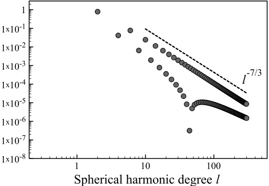
A second example illustrates intersecting line singularities. We consider the function
θ−
π 2
4/3
+cos−1(sinθcosφ)−
π 2
4/3
=cos−1z−
π 2
4/3
+cos−1y−
π 2
4/3
1 10 100
Spherical harmonic degree
1x10⁻⁸
1x10⁻⁷
1x10⁻⁶
1x10⁻⁵
1x10⁻⁴
1x10⁻³
1x10⁻²
1x10⁻¹
1 1x101
1x10² Point singularity, order 1
Line singularity, order 3/2
l
-5/2 [image:17.612.133.407.136.328.2]l
Figure 1: A comparison of the spherical harmonic spectra E(l) of a point singularity of order 1 and a line singularity of order 3/2 as defined in the text; in both casesE(l)∼l−5/2.
1 10 100
Spherical harmonic degree
1x10⁻⁸
1x10⁻⁷
1x10⁻⁶
1x10⁻⁵
1x10⁻⁴
1x10⁻³
1x10⁻²
1x10⁻¹
1
l
-7/3l
[image:17.612.129.407.403.595.2]1 10 100
Spherical harmonic degree
1x10⁻⁷ 1x10⁻⁶ 1x10⁻⁵ 1x10⁻⁴ 1x10⁻³ 1x10⁻² 1x10⁻¹ 1 1x101
a=5 a=0.5
l
-7/2 [image:18.612.129.406.131.326.2]l
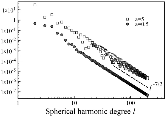
Figure 3: The spectrumE(l) off3 which has a nonlinear line singularity of order p= 5/2 on the intersection of the surface 1/2 +ay−z3= 0 with the unit spherical surface centred at the origin, for a = 1/2 and a = 5. The dashed line confirms that, for both choices ofa, the envelope scales asl−7/2.
Lastly, as addressed in the discussion, we speculate that the results per-taining to the spectral signature of a line singularity may be generalised to any closed curve on the spherical surface. To demonstrate that this a reasonable assertion, we present a third example of the function
f3(θ, φ) =|1/2 +a sinθcosφ−cosnθ|5/2,
4
Discussion
In this paper we have discussed the spherical harmonic signature of ei-ther line or point (or both) singularities, of specified order, of an oei-therwise smooth function. Line singularities are more grave than point singularities of the same order, a fact that is entirely consistent with the fact that line and point singularities are topologically distinct. The results in this paper have been proved using a mixture of asymptotic analysis and recourse to standard results. A more formal treatment of this work is almost certainly possible, perhaps by extending the analysis of [22] to associated Legendre functions and spherical harmonics.
We speculate that the spectral signature of a singularity defined on a line of colatitude (in some coordinate system) may be extended to that of a singularity on any closed curve on the spherical surface, since such a curve can be smoothly mapped to a line of colatitude. In §3 we provided a numerical example that shows the validity of this assertion in the given case. Such a generalisation may be intuitive but a proof does not appear to be straightforward. On the interval [−1,1], if f(x) has a singularity of order p at g(x0), then f(g(x)) has a singularity of order p at x0, if g is a smooth (possibly nonlinear) bijective function on [−1,1] (see Appendix A). Sincef(x) and f(g(x)) have singularities of the same order, it follows that they possess the same asymptotic scaling of (say) Legendre polynomial coefficients. This statement is equivalent to showing that
Z 1
−1
Pn(x)f(x)dx∼
Z 1
−1
Pn(x)f(g(x))dx=
Z 1
−1
Pn(g−1(y))f(y)J(y)dy
wherey=g(x) andJ is the associated Jacobian of transformation. To prove this assertion, the key problem is that, in the variable y, although f now appears untransformed,Pn(g−1(y)) are no longer Legendre polynomials and we cannot say anything further about how the integral scales withn. The same issue occurs on a spherical surface: the smooth mapping that connects any closed curve with a line of colatitude corrupts the spherical harmonics, and the results that we have derived cannot be directly applied. However, in both one and two dimensions, crude estimates of the scalings may still be obtained using integration by parts.
discriminate between the cause being a point singularity of orderlk−3/2 or a line singularity of orderlk−1. It is worth remarking that such a degeneracy is a generic issue; for example, in atmospheric turbulence it is not possible to say definitively which are the controlling singularities [12], there being two distinct scalings in the energy spectrum ofn−3andn−5/3 on different ranges of the spatial wavenumbern. Secondly, only a weakened form of Darboux’s principle could be proven here, so that the overall spectral slope supplies only a bound on any individual component singularities. This bound will not be tight if two or more singularities have spectra which sum together in such a way that a delicate cancellation takes place at leading order, leaving the total spectrum decaying faster than expected. However, this circumstance is conjectured never to arise, so that the overall spectral slope is precisely that stemming from any gravest singularity. Further work on this subject is beyond the present scope, and may be advanced by the derivation of a formal proof of Darboux’s principle in 1D.
Lastly, it is worth highlighting a particular example in which much can be learned from the energy spectrum (which is, in fact, the motivating example for this manuscript). Low-viscosity flow in a rotating spherical shell leads to shear layers on the the tangent cylinder, the axial cylinder of fluid that is tangent to the inner spherical boundary [19]. In the absence of viscosity, such shear layers become formal discontinuities. The spherical harmonic spectrum of such solutions will have a signature dictated by the order of the singularities on the tangent cylinder, which are lines of colatitude on any spherical surface. In this physical system it is likely that these are the only singularities present, so it is possible, assuming that Darboux’s principle holds in the stronger form, to discern the order of the line singularities solely from the spectrum.
Acknowledgements
A
The spectral signature of line singularities
Consider a functionf(θ, φ) that has a single line singularity of orderpwhich, in an appropriately rotated coordinate system, takes the form
f(θ, φ)∼
A+Bsgn(θ−θ0)
|θ−θ0|pg(φ) (14)
in the neighbourhood of a line of colatitudeθ=θ0∈(0, π), for some smooth g(φ), constantsAandBand realp >−1. We will show that the asymptotic form of the spherical harmonic coefficients takes the form
aml ∼e−αml−(p+1) asl, m→ ∞,
with 0< α, from which the energy spectra
E(l) =
s X
m
(aml )2 ∼l−(p+1)
follows.
Before embarking on a proof, we first show that iff(θ, φ) has a singularity of order p on θ = θ0, and if θ = h(z) is a smooth invertible (possibly nonlinear) function with θ0 = h(z0), then f(h(z), φ) has a singularity of order p on the linez =z0. That is, this smooth coordinate transformation leaves invariant the order of the singularity. Close to z = z0, θ = h(z) ∼ h(z0) + (z−z0)h0(z0) and soθ−θ0 ∼(z−z0)h0(z0). It follows that, provided h0(z0) is finite,
f(h(z), φ)∼
C+Dsgn(z−z0)
|z−z0|pg(φ),
and sof(h(z), φ) has a singularity of orderpasz→z0. Ifh0(z0) is not finite, then the singularity in the independent variablezmay take a different from that inθ (see §2.2).
To prove the result required, it is marginally easier to work with the transformed coordinate z = cosθ. The singularity in θ of order p, as de-fined above, translates into a singularity of the same order in z since the inverse cosine function, away from its end points, is smooth. The associated Legendre functions satisfy the Sturm-Liouville equation (wherez= cosθ)
where
Lmu=− d dz
(1−z2)d u dz
+ m
2
1−z2 u(z).
For a given spherical harmonic orderm, let us transform first in azimuth
fm(θ) =
Z 2π
0
f(θ, φ)
sin cos
mφ dφ. (15)
By assumption, g is smooth and so fm decays exponentially fast in m as e−αm, α > 0. It only remains to transform fm in colatitude. Since our spherical harmonics are fully normalised,
aml =
Z 1
−1
Plm(z)fm(z)dz = 1 l(l+ 1)
Z 1
−1
LmPlm(z)fm(z)dz. (16)
Let the (unique) integer sbe such that
−1< p0≤1, p0 =p−2s.
Under the assumptions on f, we can integrate by parts twice, s times [8], to find that
aml = 1
l(l+ 1)s
Z 1
−1
Lsmfm(z)Plm(z)dz. (17)
We now exploit the asymptotic behaviour of associated Legendre functions in the open interval (−1,1) [1]:
Plm(cosθ)∼
π2(δm0+ 1) 2 sinθ
−1/2 cos
(l+1/2)θ−π/4+mπ/2
+O(l−1)
(18) which, in accordance with (6), are normalised such that
Z 1
−1
Plm(z)dz2
dz ∼ π(δm0+ 1)
−1
. (19)
Provided that Ls
mfm is integrable (as we shall justify shortly), and noting from (18) thatPlm(cosθ) sinθ is bounded forl1, it follows that
|aml | ≤ 1 l(l+ 1)s
Z π
0
|Lms fm(cosθ)| |Plm(cosθ) sinθ|dθ≤C l
−2s. (20)
The function Ls
end points,z=±1, due to repeated multiplications by the factor 1/(1−z2) inLs
m. However, fm is not just any function: sincef is smooth away from the singular line, fm must behave as sinmθ as θ→ 0, π [5] and in fact the end points present no trouble. Indeed, writingfm(z) = (1−z2)m/2w(z) for somew(z),
Lm
(1−z2)m/2w(z)
= (1−z2)m/2
(z2−1)w00(z)+2(1+k)z w0(z)+m(m+1)w(z)
.
(21) so that Lmfm also has an mth order zero; iterating, we see that Lsmfm(z) does as well and so remains regular atz=±1.
To tighten the bound on aml from l−2s (20), we now use (18) again. In view of the quasi-trigonometric form of (18), one might be tempted to apply directly the Fourier convergence theory, summarised in the introduction, to (14). However, this is not possible, due primarily to the error term in (18), swamping any scaling that decays more rapidly thanO(l−1). We therefore only use (18) to tighten the scaling we already have.
We divide the remaining analysis into two cases depending on the sign of p0. Let us denote Ls
mfm(z) = qm(z), where qm(z) has a zero of orderm atz=±1 and a singularity of order−1< p0 ≤1 at cosθ0.
Case I: −1< p0 ≤0
Direct substitution of (18) into (17) gives
(l(l+ 1))sam l
C ∼
Z π
0
qm(cosθ) √
sinθcos
(l+ 1/2)θ−π 4+
mπ 2
dθ+O(l−1),
(22) whereC = π2(δm0+ 1)/2
−1/2
. Formally, since the asymptotic expansion is valid only away from the end points, we should restrict attention to the interval [−1+,1−] for some 0< 1, modifying the limits of integration in (22). However, in view of the non-singular nature of the integrand in (22) near the end points, we may take to be so small so that the error incurred by altering the interval to [−1,1] can be neglected. The function qm(cosθ)
√
sinθ is smooth except for (i) a zero of order m+ 1/2 at θ = 0 and (ii) a singularity atθ0 of orderp0≤0. Since the singularity (ii) is more potent than (i), it therefore dominates the spectrum. Furthermore, noting that the above is just a (shifted) cosine transform, we may appeal to the Fourier results summarised in the introduction to see that, for someα >0,
Case II: 0< p0 ≤1
We cannot use the same argument as above as not only might the zero of order m+ 1/2 at θ = 0 have a stronger influence than the singularity at θ0, but l−(p
0+1)
< l−1 and the dominating error term means that we cannot do better than the bound l−2s−1. Instead we integrate (17) by parts once (rather than twice) to find
(l(l+1))saml = 1 l(l+ 1)
Z 1
−1
(1−z2)dqm(z) dz
dPlm(z) dz dz+
m2 l(l+ 1)
Z 1
−1
qm(z)Plm(z) 1−z2 dz
the boundary term vanishing as both qm and dPlm/dz are nonsingular at z=±1 and everywhere continuous. Now we use the recurrence [1, 8.5.4]
(1−z2)dP m l
dz =Q(l) (l+m)P m
l−1−lzPlm∼l(Plm−1−zPlm)
if l m, which has been adjusted to take into account the normalisation (19) by inserting the algebraic factor Q(l), where Q(l) → 1 as l → ∞. It follows that, whenlm:
(l(l+1))saml ∼ 1 (l+ 1)
Z 1
−1
dqm(z)
dz P
m
l−1−zPlm
dz+ m 2
l(l+ 1)
Z 1
−1
qm(z)Plm(z) 1−z2 dz.
Since dqm/dz has a singularity of order p0 −1 with −1 < p0 −1 ≤ 0, it follows that by appealing to case I, the first integral (without the prefactor) scales as l−((p0−1)+1)). The second integral (without the prefactor) scales algebraically inlwith exponent either−(p0+ 1) or−1 (from the error term in (18)), which ever is the greater. Sincep0 >0 then the entire second term scales as l−3. Note that despite the factor of (1−z2) in the denominator, this integral always exists: if m = 0 then it is trivially zero; if m > 0 then both Plm and qm behave like (1−z2)m/2 as z → ±1 and so the integrand is everywhere finite. Since the entire first term scales as l−(p0+1), it follows thataml ∼e−αml−2s−p0−1 =e−αm l−(p+1),α >0.
The entire analysis can be generalised to the case with singularities of the form (A+Bsgn(θ−θ0))|θ−θ0|plog|θ−θ0|q, by applying standard Fourier results [18; 5]. In such a case,aml ∼e−αml−(p+1)logql,α >0.
Lastly, we show that the energy spectra, binned per degree l, takes the form
E(l) =
s X
m
as l → ∞ when aml ∼ e−αmf(l) for some dependence f(l). Since the sum overm converges exponentially, its sum scales independently ofl:
E(l)2 ∼f2(l) l
X
m=0
e−2αm ∼f2(l)1−e
−2αl
1−e−2α ∼f 2(l),
and the result follows.
B
Application of approximation theory
We summarise here some relevant results from approximation theory that somewhat parallel the development given in the paper. For ease of expla-nation, we frame most of the discussion in terms of a Legendre polynomial representation in 1D. We consider on the interval [−1,1]
R(N)2 =
Z 1
−1
u(x)−PNu
2
dx=
∞ X
n=N+1
a2n, (23)
a measure of the residual incurred in approximatingu by its truncated ex-pansion in (fully normalised) Legendre polynomials to degreeN,
PN =
PN
n=0anPn(x). Let us define
kfk2Hm =
m
X
r=0
Z 1
−1
drf dxr
2
dx,
the Sobolev norm of f involving derivatives of up to degree m. It may be shown that
R(N)≤CN−mkukHm (24)
for anym for which kuk2
Hm exists [9; 8], placing algebraic bounds onR(N)
depending on the differentiability ofu. Using space interpolation, it is pos-sible to extend this bound to non-integer values of m, which may also be generalised to approximations in other orthogonal polynomials.
Taking the supremum of these values (assuming C is independent of m) leads toR(N)≤C N−(p+1/2).
This bound for R(N) is entirely consistent with that for aN ∼N−(p+1). Since aN converges at only an algebraic rate, aN/aN+1 → 1 as N → ∞ from which it follows that aN/aN+n → 1 for any integer n >0 and so all an,n > N, asymptotically “equally contribute” to the residual. ThusR(N) must decay slower than any particular an. Note that, should an converge exponentially inn, thenR(N) would be well approximated byaN+1 and we would anticipate thatR(N)∼aN.
These one-dimensional results have exact counterparts for functions de-fined on a spherical surface. It may be shown that
R(L) =
v u u t I
|f(θ, φ)− L
X
l=0 l
X
m=0 am
l Ylm|2dΩ≤CL
−mkfk Hm
whereHm is defined in an analogous manner [14]. For functions which have singularities on lines of colatitude of the form |θ−θ0|p, we may therefore infer the boundR(L)≤C L−(p+1/2).
References
[1] M. Abramowitz and I. A. Stegun, Pocketbook of mathematical
functions, Verlag Harri Deutsch, 1984.
[2] G. Backus, R. Parker, and C. Constable, Foundations of
Geo-magnetism, CUP, 1996.
[3] M. Bain,On the Uniform Convergence of Generalized Fourier Series, J. Inst. Maths. Applics., 21 (1978), pp. 379–386.
[4] C. Blakely, A. Gelb, and A. Navarra, An automated method
for recovering piecewise smooth functions on spheres free from Gibbs oscillations, Sampling Theory in Signal and Image Processing, 6 (2007), pp. 323–346.
[5] J. P. Boyd,Chebyshev and Fourier Spectral Methods, Dover, 2001.
[7] J. P. Boyd,Large-degree asymptotics and exponential asymptotics for Fourier, Chebyshev and Hermite coefficients and Fourier transforms, J. Eng. Math., 63 (2009), pp. 355–399.
[8] C. Canuto, M. Y. Hussaini, A. Quarteroni, and T. A. Zang,
Spectral Methods: Fundamentals in Single Domains, Springer, 2006.
[9] C. Canuto and A. Quarteroni,Approximation results for
orthogo-nal polynomials in Sobolev spaces, Math. Comp., 38 (1982), pp. 67–86.
[10] D. Elliott,The Evaluation and Estimation of the Coefficients in the Chebyshev Series Expansion of a Function, Math. Comp., 18 (1964), pp. 274–284.
[11] L. Fox and I. B. Parker,Chebyshev Polynomials in Numerical Anal-ysis, Oxford University Press, London, 1968.
[12] K. S. Gage and G. D. Nastrom, Theoretical interpretation of
at-mospheric wave number spectra of wind and temperature observed by commercial aircraft during GASP, J. Atmos. Sci., 43 (1986), pp. 729– 740.
[13] A. Gelb, The resolution of the Gibbs phenomenon for spherical har-monics, Math. Comp., 66 (1997), pp. 699–717.
[14] B.-Y. Guo,Spectral Methods and Their Applications, World Scientific Publishing, 1998.
[15] A. Jackson, Bounding the long wavelength crustal magnetic field, Phys. Earth Planet. Int., 98 (1996), pp. 283–302.
[16] M. K. Jain and M. M. Chawla, Estimation of the Coefficients in
the Legendre Series Expansion of a Function, J. Maths. Phys. Sci., 1 (1967), pp. 247–260.
[17] M. Kzaz, Asymptotic expansion of Fourier coefficients associated to functions with low continuity, J. Comput. Appl. Math., 114 (2000), pp. 217–230.
[18] M. J. Lighthill, Introduction to Fourier Analysis and Generalised Functions, Cambridge University Press, 1958.
[19] P. Livermore and R. Hollerbach,Successive elimination of shear
[20] K. O. Mead and L. M. Delves,On the Convergence Rate of Gener-alized Fourier Expansions, J. Inst. Maths. Applics., 12 (1973), pp. 247– 259.
[21] S. A. Orszag, Fourier-series on spheres, Mon. Weather Rev., 102 (1974), pp. 56–75.
[22] A. Sidi,Asymptotic expansions of Legendre series coefficients for func-tions with interior and endpoint singularities, Math. Comp., 80 (2011), pp. 1663–1684.
[23] G. Szeg¨o,Orthogonal polynomials, vol. 1, American Mathematical So-ciety, 4th ed., 1975.
[24] D. Viswanath and S. S¸ahuto˘glu, Complex singularities and the Lorenz attractor, SIAM Rev., 52 (2010), pp. 478–495.