Modelling of hydraulic fracturing process by coupled discrete element and fluid dynamic methods

White Rose Research Online URL for this paper:

http://eprints.whiterose.ac.uk/81450/

Version: Accepted Version

Article:

Sousani, M, Eshiet, K, Ingham, D et al. (2 more authors) (2014) Modelling of hydraulic

fracturing process by coupled discrete element and fluid dynamic methods. Environmental

Earth Sciences, 72 (9). 3383 - 3399. ISSN 1866-6280

https://doi.org/10.1007/s12665-014-3244-3

eprints@whiterose.ac.uk https://eprints.whiterose.ac.uk/ Reuse

Unless indicated otherwise, fulltext items are protected by copyright with all rights reserved. The copyright exception in section 29 of the Copyright, Designs and Patents Act 1988 allows the making of a single copy solely for the purpose of non-commercial research or private study within the limits of fair dealing. The publisher or other rights-holder may allow further reproduction and re-use of this version - refer to the White Rose Research Online record for this item. Where records identify the publisher as the copyright holder, users can verify any specific terms of use on the publisher’s website.

Takedown

If you consider content in White Rose Research Online to be in breach of UK law, please notify us by

Modelling of hydraulic fracturing process by coupled discrete

element and fluid dynamic methods

Sousani Marina

, Eshiet Kenneth

, Ingham Derek

, Pourkashanian Mohamed

,

Sheng Yong

1 _{University of Leeds, Energy Technology and Innovation Initiative (ETII), Leeds, LS2 9JT, UK}

2 _{University of Leeds, School of Civil Engineering, LS2 9JT, UK}

*_{Corresponding author. Sheng Yong Tel: +44 (0)113 3433200; fax: +44 (0)113 3432265; email:}

y.sheng@leeds.ac.uk

Abstract

A three-dimensional model is presented and used to reproduce the laboratory hydraulic fracturing test performed on a thick-walled hollow cylinder limestone sample. This work aims to investigate the implications of the fluid flow on the behaviour of the micro structure of the rock sample, including the material strength, its elastic constants and the initialisation and propagation of fractures. The replication of the laboratory test conditions has been performed based on the coupled Discrete Element Method and Computational Fluid Dynamics scheme. The numerical results are in good agreement with the experimental data, both qualitatively and quantitatively. The developed model closely validates the overall behaviour of the laboratory sample, providing a realistic overview of the cracking propagation towards total collapse as well as complying with Lame’s theory for thick walled cylinders. This research aims to provide some insight into designing an accurate DEM model of a fracturing rock that can be used to predict its geo-mechanical behaviour during Enhanced Oil Recovery (EOR) applications.

Keywords

gas industry (Jin 2012). However, underground conditions constitute a field of multiple variables which still remain to be extensively investigated.

Enhanced Oil Recovery (EOR) is regarded as one of the effective schemes for a low-carbon energy future, as it

can inject CO2 underground and extract more oil from hydrocarbon reservoirs at the same time (Blunt et al.

1993; Parker et al. 2009; Jin 2012). However the whole process requires a considerable pressure in order to

introduce liquefied CO2 underground, thus causing redistribution of the in-situ effective stresses within the

reservoir. Although in EOR fracturing of the oil reservoir is desirable, such stress changes may induce irreversibility to the rock strata, thus causing possible reactivation of the existing faults leading to possible

leakage of CO2(IEAGHG 2011b; Wilkins and Naruk 2007). Therefore valid estimates of the mechanical

behaviour of the rock material under intense injection conditions are crucial to the efficient planning and operation of petroleum reservoirs.

Extended research has been performed to investigate the wellbore instability for hard and low porosity sedimentary rocks (Zhang et al. 1999; Jaeger et al. 2009), as well as permeability changes of rocks with the in-situ stress changes (Holt 1990; Bachu and Bennion 2008; Bouteca. M. J. 2000; Bruno 1994; Bryant et al. 1993; Ferfera et al. 1997). Furthermore mathematical solutions and experimental models have been developed to look into the critical mechanical parameters, such as the stress envelope and crack network, or the way that these are influenced by the induced stress regime (Aminuddin N. J. 2011; Ziqiong Z. 1989; Eslami J. 2010; Hanson et al. 1980). However, while there are some studies dealing with modelling and simulation of rocks in the micro-scale (Gil 2005; Tomiczek 2003; Akram 2009; Potyondy 2004; Li 2001; Funatsu 2007; Kenneth et al. 2013; Martinez 2012) the complex interplay between the micro-properties of a virtual sample and their corresponding effect on the material’s behaviour during the calibration procedure provides a general guidance at best. Part of this study deals with the adopted methods and even though the description of the way values of the calibration procedure was obtained is given in summary, it may serve as future reference for other researchers.

The DEM (Discrete Element Method) approach was utilised to simulate the behaviour of granular materials such as sandstone and limestone, with discontinuities such as joints, fractures, and/or faults and the fluid-solid interactions among them (Potyondy 2004; Walton 1987; Chang 1987). The Lattice-Boltzmann method of computing fluid flow solves the discretised form of the Boltzmann equation which is based on the Navier-Stokes equation (Chen 1998). Other methods of computing fluid flow include Direct Numerical Simulation (DNS) (Dong 2007; Moin 1998) and Computational Fluid Dynamics (CFD). The need to provide linkages between co-existing fluid and solid phases necessitates a coupling of these techniques with the modelling of solid mechanics such as DEM. The Lattice-Boltzmann and DEM coupling is illustrated in (Boutt 2007), while approaches that incorporate CFD with DEM are presented (Xu and Yu 1997; Tsuji et al. 1993). Most of these coupling schemes are applied to granular or un-cohesive materials and in cases where the domain is dominated by fluid phases. Therefore, phenomena such as the deformation of the solid material and fracturing are not captured due to either the limitation of the coupling technique or the delineation of study. This study also deals with the fluid-solid interaction incorporating the DEM technique and the PFC3D computer package developed by Itasca (Itasca-Consulting-Group 2008a) and an extension of its applicability via the modelling of hollow-cylinder laboratory tests. Applications of this sort, where direct numerical and experimental comparisons were carried out, are still lacking.

In the PFC3D model, the particles are connected by parallel bonds replicating the cementation between grains in actual rocks. The macroscopic behaviour of the material is derived from statistical assumption of the interactions between the particles of the assembly used to represent the rock sample. Hence large particle numbers will provide more accurate results. However the simulation time was a key limitation, given the available computer processing power. At the moment, computer packages using DEM to study rock

micro-parameters are restricted to about 5×105 spherical particles for high powered desktop computing.

2

Hydraulic fracturing experiment

a number of tests were conducted on a series of synthetic and natural rock samples subjected to differing operating and boundary conditions. Artificial samples were created to imitate soft permeable rocks that are low in strength (bonded glass bead materials), while the natural samples consisted of limestone. The early and non-progressive collapse, meaning the sudden disintegration of the synthetic samples during the initial stages of fluid flow, illustrates the combined effects of permeability and strength on the failure mode. This phenomenon is not observed in the limestone samples which are less permeable but have a higher strength. Observed occurrences of pressure build-up, deformation and fracturing during the tests show the role of an operating well and reservoir conditions as well as the physical and mechanical properties of materials on mechanisms that result in collapse failure and the mode of application of injected water inside the sample.

To determine the mechanical behaviour of natural rock under prescribed fluid flow conditions, a set of tests was conducted on a cylindrical limestone sample (37.8mm diameter and 100mm height) which was drilled along its axis to create a cylindrical cavity. The test was performed on a specimen with a cylindrical cavity of 21.5mm sourced from Tadcaster, North Yorkshire, U.K. An initial pressure differential was established between the outside of the specimen and the hollow centre, which was kept at zero pressure. The outer boundary fluid pressure was then gradually increased until failure. The laboratory equipment for the fracturing test included a permeameter combined with a CT scanner and hydraulic hand pumps in order to drive and regulate the injection fluid at the prescribed pressure through the specimen cavity and around the circumference of the specimen. A set of computers to monitor and control test operations as well as to process the scan images were also included.

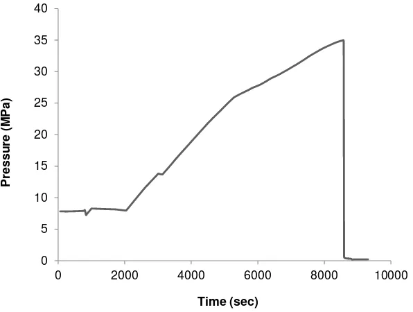
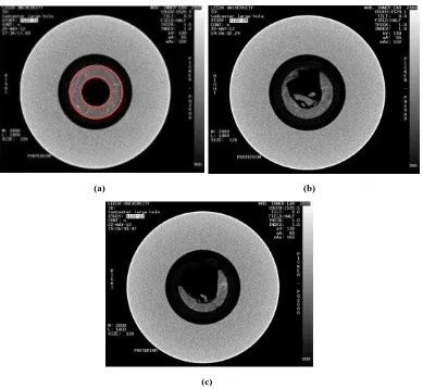
Fracture initiation was observed to occur after about 8000sec and the eventual collapse of the cavity wall occurred at 5056 Psi (35MPa) followed by a rapid drop in the circumferential pressure to 29 Psi (Fig. 1). The initial state of the specimen and the progressive fracturing and collapse is illustrated in Fig. 2.

Fig. 1 Fluid pressure differential between the hollow core and the outer surface of the slice, versus time. Maximum fluid pressure differential 35MPa.

0 5 10 15 20 25 30 35 40

0 2000 4000 6000 8000 10000

P

re

s

s

ure

(M

P

a

)

(a) (b)

(c)

Fig. 2 Scan image of the large cavity limestone specimen inside the test-tube (a) in the initial state (red), and

(b), (c) in various stages of the collapse of the cavity wall.

3

Simulated experiment

3.1

Determination of micro-parameters and sample calibration

This test is built upon the Uniaxial and the Brazilian procedures using the 3D version of PFC. A rectangular model is used to replicate the limestone rock sample tested in the Laboratory of the University of Leeds as previously discussed. The aim of the test is to calibrate the PFC model by matching its maximum Uniaxial

Compressive Strength (UCS), tensile strength and elastic properties (Young’s modulus E and Poisson’s ratio v)

with the ones of the laboratory sample obtained from literature. The calibration process includes a series of simulated Uniaxial and Brazilian tests in order to investigate and identify the micro-parameters critical to the overall mechanical behaviour of the numerical model.

The DEM method used in this work to represent the solid body of the real rock and its short-term behaviour, was based on the characterization of the virtual specimen in terms of parameters in the micro-scale (Itasca-Consulting-Group 2008c). More specifically the properties of UCS/tensile strength and elastic constants are macroscopic properties and they cannot be directly described in a DEM model, thus a micro-property process

had to be set. This involved the relation between the deformability and strength of the assembly (Young’s

modulus, angle of friction, Poisson’s ratio and strength for particles and bonds) as shown in Table 2, to their

equivalent set of macro-responses.

During each Uniaxial test the specimen was axially compressed by two walls acting as loading platens (Fig.3), whereas the sample was compressed laterally during the Brazilian test (Fig.5). The results obtained were monitored and recorded by three different measurement schemes: specimen-based, wall-based (corrected) and measurement circle-based. The basic difference between the first two schemes is that the specimen-based results are based solely on the observed total stresses and strains applied on the confining walls, whereas in the second case the results are derived from measurements at each wall contact point, where the effect of possible ball-wall overlap has been removed. Finally, the measurement of the circle-based quantities are derived from three measurement circles located in the upper, central and lower portions of the specimen and provide a more uniform averaged response over the entire specimen surface thus were chosen as the best measurement technique for this work.

3.1.1

Uniaxial test with PFC3D

In the simulated Uniaxial test a rectangular specimen of dimensions 37.8×37.8×100mm (Fig. 3) was generated by a standard sample genesis procedure, were the synthetic material consisting of particles and cementation (parallel bonds) is produced in a vessel. The vessel consists of frictionless walls in the X, Y and Z directions forming an isotropic and well-connected virtual assembly. Next the lateral walls were removed and before enabling the movement of the top and bottom platens, the assembly was cycled in order to absorb any residual forces that the lateral walls were acting on the sample (Fig.3-left). The top and bottom walls were used as the loading platens and assigned a constant speed before initiating the test (Fig.3-right). In order to represent the real environment of an underground rock sample more realistically, the specimen is initially compressed before the

test begins at Pc=0.1MPa pressure. The loading platens are considered frictionless and with stiffness much

Fig. 3 Schematic of the virtual limestone assembly during the standard genesis procedure (left). In Uniaxial test the sample is loaded by platens moving towards each other at constant speed (right).

Due to lack of appropriate documentation regarding the properties of the laboratory limestone sample, it was considered necessary to obtain the relevant properties from literature. The UCS, tensile strength and the elastic constants of a real limestone sample from existing literature are summarised in Table 1. The laboratory limestone sample was a moderately weak one, thus a maximum UCS strength near the lower part of the strength range reported in literature was sought after for the simulation model.

Table 1 Typical geo-mechanical properties of limestone, according to the literature(University-of-Stanford ;

Knill 1970; Hallsworth 1999)

Limestone parameters

UCS strength q = 30-250MPa

Tensile strength = 5-25MPa

Young’s modulus E = 15-55GPa

Poisson’s ratio v = 0.18-0.33

Grain size 0.6-2.0mm

Density 2500-2700kg/cm3

Porosity 5-30%

Initially both the Young’s modulus of the particles and bonds were set to 40GPa, according to the conclusions of

Akram and Sharrock (Akram 2009). Depending on their findings, the Young’s modulus of the particles is in

good agreement with the Young’s modulus of the bonds, as long as the stiffness ratio is about 1.0. Even though the referring sample was sandstone, it appears to be appropriate to use this finding in the case of limestone. This is because the two types of rocks are similar and the ratio of the normal and shear stiffnesses was also 1.0. A few trials indicated that the aforementioned micro-parameters should change taking the final value of the Young’s modulus of the particles should be =30GPa, whereas the Young’s modulus of the parallel bonds

should be =20GPa, lying within the broad range 15-55GPa (Table 1). Although there is no guideline

(1)

It is used in order to reduce possible unbalanced forces and locked-in stresses (tensile and compressive) during the generation process and provide better internal equilibrium to the assembly. Thus in this case it was set to be one tenth less than the desired Uniaxial maximum strength. Next, the Poisson ratio was set by defining the ratio of the shear to the normal contact stiffness for both the particles and bonds. A few iterations were carried out in order to match these micro-properties with the corresponding elastic constants of the material. Once the elastic constants had been matched, the maximum strength of bonds was set near a low desired value within the range 30-250MPa. A large number of trials had to be executed in order to finally match and reproduce the relevant behaviour of a limestone rock. Table 2 demonstrates the complete set of input data used for the Uniaxial test.

Table 2 PFC micro-parameters used for the Uniaxial simulated test on the limestone model

Micro-parameters that define the sample

Sample height (mm) 100

Sample diameter (mm) 37.8

Sample porosity (%) 15

Initial friction of balls 5.5°

Gravity (m/s2) 9.81

Micro-parameters that define the particles

Ball radius (mm) 0.85

Ball density (kg/m3) 2600

Young’s modulus (GPa) 30

Ball stiffness ratio 1.0

Required isotropic stress (MPa) 0.4

Micro-parameters that define parallel bonds

Radius multiplier 1.0

Young’s modulus (GPa) 20

Normal/Shear stiffness ratio (Pa/m) 1.4

Normal strength (MPa) 30

Std. deviation of normal strength 30 104

Shear strength (MPa) 30

Std. deviation of shear strength 30 104

The test was performed with a velocity of up=0.005m/s and the axial stress ( ) was continuously monitored

rising to a maximum value and then decreasing as the sample fails. It was terminated when the current value of the sample’s axial stress became less than 0.01 times the previously recorded maximum axial stress value

( ). Using this configuration, the sample showed the expected behaviour in terms of the

Fig. 4 PFC3D output of the stress versus strain for the limestone assembly used in the simulated Uniaxial test.

Fig.4 clearly indicates that the stress-strain relationship is approximately linear, thus showing that the material is in its elastic regime, until it reaches the point of its ultimate axial strength (46MPa). Beyond that point, the material enters the plastic deformation regime, indicating irreversible damage. Table 3 highlights the results obtained from the Uniaxial test indicating that the material is weak in terms of both the UCS strength and its

elastic constants. Further, the Poisson’s ratio and the Young’s modulus are well within the reported range for

limestone formations.

Table 3 Uniaxial test results of the UCS strength and the elastic constants for the weak simulated limestone

model.

Uniaxial results (moderately weak sample)

Elastic constants E=34GPa

v=0.21

UCS strength =46MPa

3.1.2

Brazilian test with PFC 3D

In the simulated Brazilian test the virtual specimen was a cylindrical disc with the same micro-properties obtained from the aforementioned rectangular specimen used in the Uniaxial test (Table 2). A well-connected assembly of uniform size particles was created with genesis procedure and the required stresses were applied so that the sample reached the target isotropic stress. The specimen then was trimmed into a cylindrical disc of 50mm diameter and 30mm thickness, comprised of 12162 particles. The disc was in contact with the lateral walls in the X direction, whereas both the walls in the Y and Z directions were moved apart by a distance of 0.05×height of initial rectangular assembly and 0.05×diameter of the disc. During the test the Y and Z walls had zero velocity whereas the X-lateral walls were moving towards each other using the same platen-loading logic described in the Uniaxial test Fig.(5).

0 5 10 15 20 25 30 35 40 45 50

0.00 0.50 1.00 1.50 2.00 2.50

UC

S

s

trengt

h (M

P

a

)

Figure 5 Schematic of PFC Brazilian disc (Itasca-Consulting-Group 2008c).

During the test the force (F) acting on the sample initiating by the movement of the X-lateral walls was calculated and the maximum value was recorded reaching a maximum value and then decreasing as the sample failed. The same termination criterion, as in the Uniaxial test, was used therefore the test was terminated when the current average force became smaller than 0.01times the previously recorded maximum force (

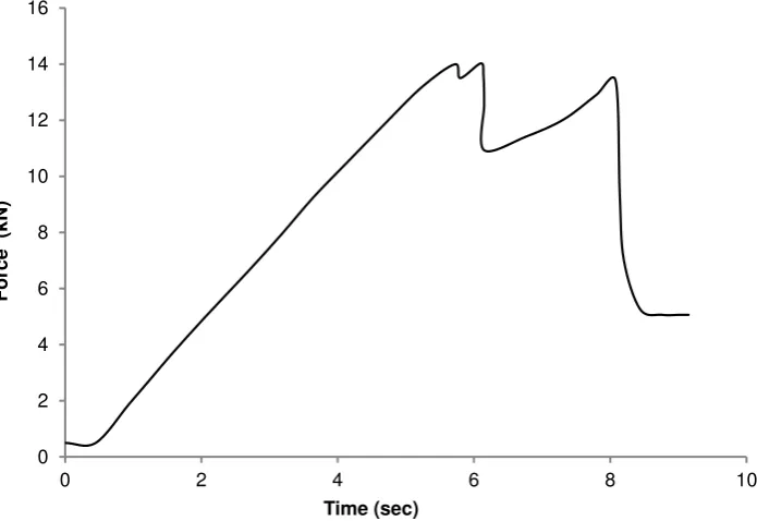
). Fig.6 demonstrates the behaviour of the material until it reaches the ductile area and the point of its peak force 14KN. When a cylindrical sample is subjected in a compressive loading perpendicular to its axis and in a diametrical plane, it fails under tension (Wright 1955). The Brazilian tensile strength (6MPa) is calculated by

(1)

Where is the peak force acting on the platens and and are the radius and the thickness of the virtual

disc respectively.

Figure 6 Force acting on the platens of the Brazilian disc versus time. The sample fails under 14kN.

4

Hollow cylinder test

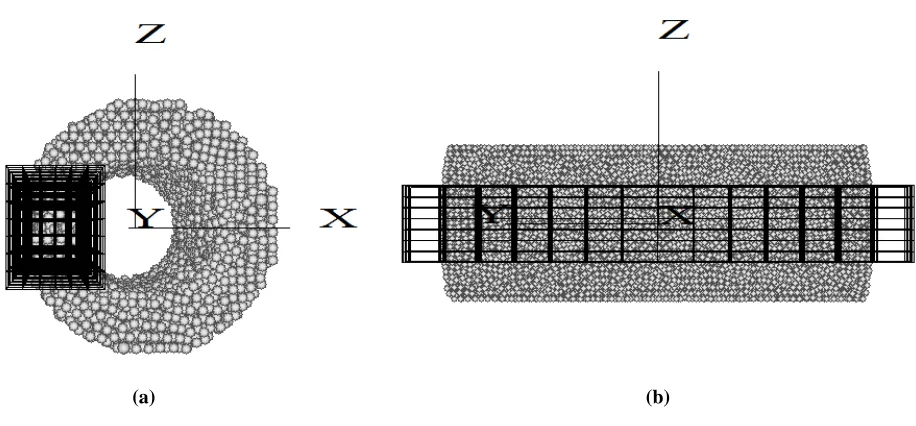
Even though hollow cylinder tests are commonly used in studies pertaining to wellbore instability and sand production nonetheless, they are also used to investigate fracturing processes (Ewy 1988; Elkadi 2004; Enever 2001; Ayob 2009). As the mode of fluid application is a major determinant of the rock material behaviour, the simulated hollow cylinder test replicates the laboratory fracture test exploring the stress regime and the propagation of cracks. The virtual model was cylindrical with dimensions of diameter 37.8mm, length 50mm and comprised 12840 particles of uniform size (Fig. 7). It is important to point out that although a PFC model in general demonstrates similar behaviour with that of a real rock, we do not correlate a PFC particle with a real rock grain. The virtual sample itself is a precise micro-structural assembly in its own right and should not be associated with the micro-structure of a rock (Itasca-Consulting-Group 2008c). The model has a hollow central region (pipe-like) with a diameter of 21.3mm, along the axis of the cylinder following the layout of the laboratory sample.

During the laboratory experiment, the rock sample was placed inside a tube through which water was injected. The movement of the fluid through the body of the sample was activated by setting a pressure difference between the outer perimeter of the sample and its internal hollow core. The purpose of the hollow core was to

allow the fluid’s movement through the pipe to make the rock fully saturated keeping its internal pressure close

to zero, while the external pressure was gradually increased. This pressure difference forced the fluid to radially penetrate the rock’s body towards its core.

0 2 4 6 8 10 12 14 16

0 2 4 6 8 10

Forc

e

(kN)

Figure 7 Schematic of the virtual limestone model with a hollow cylindrical core.

The fluid-flow logic was used for this work as a function already developed by the Itasca Company (Itasca-Consulting-Group 2008a). It can be considered as a two way couple as the fluid injection has altered the structure of the rock (in terms of fractures) and the fracturing also altered the path of the fluid flow. As the problem simulated in this paper is not diluted particle flow in a fluid, but instead, it is a densely pack medium with flow pass through it pores, the particle fluid rate has no significant impact on the model.

Figure 8 The 3D mesh (filter) used to support the sample. Each side of the mesh consists of horizontal and

vertical 1D walls.

Moreover a fluid cell grid was also applied to the rectangular slice of the assembly covering the outer perimeter and the inner hollow core of the model, as illustrated in Fig.9. The whole assembly may be considered to consist of eight (8) of these slices. Since the actual laboratory experiment had radial symmetry (water flowing from the outside towards the inside in all directions along the z-x plane), it is valid to state that the flow through each

slice should correspond to approximately 1/8th of the total flow through the complete assembly. The parameters

defining the grid were its dimensions and the number of cells along each direction. There are no guidelines of the grid’s parameters other than in case of a porous medium the cells should have a size comparable to that of a few particles. This is due to the fact that porosity and permeability are calculated through each cell, thus the cell grid must be coarse. During this test 240 fluid cells were created, each with a cell size of 2.6×8.3×1.26mm. In the laboratory experiment, the sample was placed inside a tube where the fluid pressure was applied uniformly

around the outer surface of the body of the rock. Therefore, the exerted forces at each point of the rock’s outer

(a) (b)

Figure 9 Application of the fluid cell grid around a slice of the sample, (a) front view, and (b) side view

The pressure differential applied during the laboratory experiment was gradually increased starting from 8MPa with a loading rate of 0.004MPa/sec until the failure of the sample in a time frame of about 8400sec. In order to replicate the laboratory pressure inside the simulated test, the plot of the fluid pressure versus time, was divided into two regions, covering the periods of time 0 to 2000sec, and 2000 to 8400sec, as shown in Fig. 8 (dashed). In the first region, the simulated fluid pressure was set to 8MPa, which is the average of the plot points in that section (Fig. 8 solid black). In the second region of the plot, the pressure was gradually increased from 8MPa until failure.

0 5 10 15 20 25 30 35 40

P

re

s

s

ure

(M

P

a

The small timestep inherent in the PFC simulations in order to ensure stability (typically of the order of tens of microseconds) resulted in impractical computational run-times when attempting to model the complete 8400sec experiment. To alleviate this, the simulated time of the test had to be scaled down to a feasible value. The overall runtime of the shortened test was around 125sec, with the stable pressure region spanning for 25sec (=1/4 of total runtime) which corresponds to the 2000sec region of the physical laboratory experiment (=1/4 of the total 8362sec runtime). Due to the fact that the overall time of the test had to be scaled down the loading rate had to be scaled up in order for the physical and simulated tests to be equivalent, thus the pressure gradient was set to 0.12MPa/sec. Even though in reality the increase of the pressure gradient will have an effect on the overall strength of the rock, in the case of the PFC assembly the Navier-Stokes equation for incompressible fluid flow is pressure-free since there is no explicit mechanism for advancing the pressure in time. Furthermore the pressure gradient is not included in the formula thus does not affect the behaviour of the virtual assembly. Numerical tests had been carried out to confirm that this increase of loading rate has very little influence on the material behaviour of the sample.

(a)

(b)

Figure 11 (a) Simulated flow rate versus time for 13MPa (solid black) and 30MPa (dashed) constant pressure

differential between the outer and inner perimeters of the limestone assembly, and (b) applied fluid pressure versus time during the simulation of the single phase flow through the limestone sample. The pressure is kept at 8MPa for 25seconds before starting to rise in steps of 1.2MPa every 10 seconds. Sample failure occurs at

0.00 0.20 0.40 0.60 0.80 1.00 1.20

0.00 2.00 4.00 6.00 8.00 10.00

S im ula ted v olume tric flow ra te (m 3/s ) -10 -2 Time (sec) 8.00 13.00 18.00 23.00 28.00 33.00 38.00

0 20 40 60 80 100 120

to replicate the actual laboratory experiment in PFC the assumption that the fluid travels along the X axis had to be made.

Figure 12 Fluid pressure boundary conditions for the PFC model under the assumption that the movement of

the fluid is horizontal. The pressure on the outer perimeter of the model in constantly increased, whereas the pressure inside the cavity is zero.

4.1

4.1

Numerical solutions to the hollow cylinder test

The aim of the hollow cylinder test was to replicate the laboratory loading conditions on a cylindrical limestone sample with a hollow core. The test provides an indication of the stress field of the PFC model and the overall

behaviour of the assembly under high pressure differential. The equations are known as Lame’s equations

(University-of-Washington ; Perry and Aboudi 2003; Ayob 2009) and they are used to determine the stresses in thick wall cylindrical pressure vessels (Fig.13).

Figure 13 Two dimensional schematic of a hollow cylinder and an element at radius r from the centre of the

cylinder (University-of-Washington).

These are given by the following equations:

(2)

(3)

(4)

(5)

Substituting Eq.(4), (5) into (2) and (3) we conclude

(6)

(7)

For the longitudinal stress acting on the cut of the cylinder, force equilibrium law is used where a pressure

acts on an area and a pressure acts on an area , thus the overall stress acts on the area

and is given by:

(8)

For the case of a closed ends cylinder with zero internal pressure and internal radius, external pressure

and external radius, the stresses at a given distance are given by:

, , (9)

where and are the tangential, radial and longitudinal respectively.

4.2

Numerical solutions for the hydraulic fracturing test

The aim of the fluid flow test in three dimensions is to replicate the laboratory hydraulic fracturing test of the

cylindrical limestone sample. The test gives a good indication of the material’s hydraulic conductivity and the

behaviour of the sample under high pressure. The flow rate, in m3/sec, for the liquid flow through the porous media is given by

(10)

where is the cross sectional area perpendicular to the direction of flow, and is the velocity of the liquid given by Darcy’s Law (Dullien 1979; Nield 2006):

(11)

where is the absolute permeability of the sample, is the fluid’s dynamic viscosity, _P is the fluid pressure,

of Eq.(4) is the only one acting. Furthermore, local non-viscous damping is provided by PFC3D meaning that body forces approach zero for steady motion

In steady-state, the velocity in Eq.(11) becomes the interstitial velocity of the fluid. This can be derived

from the combination of the well-known Navier-Stokes and Erqun’s relations, Eq.(12) and Eq.(13) respectively

for fluid flow through packed bed which for the case of a fixed homogeneous porous material takes the form (Itasca-Consulting-Group 2008a) (University-of-Washington ; Jia 2009):

(12)

(13)

Where, is the viscosity of the fluid, is the porosity, f is the body force per unit volume, the interstitial fluid

velocity is denoted as is the height of the bed, is the pressure difference, is the mean particle

diameter, and 150 and 1.75 are constants obtained by experimentation.

As already mentioned in the Uniaxial test, during the typical generation process the sample is packed with particles of uniform size. At this stage the assembly is reaching equilibrium with the use of some stabilizing strategies (i.e. target isotropic stress) thus all body forces acting on the particles prior to fluid movement are being eliminated. In the fluid- scheme of PFC3D, driving forces from fluid flow are applied to particles as body forces, making the body force of Eq.(12) the only one acting. Furthermore, local non-viscous damping is provided by PFC3D meaning that body forces approach zero for steady motion. If we assume that the assembly of particles is similar to a packed bed, then when there is no flow through the packed bed the net gravitational force (including buoyancy) acts downward. When the flow starts moving upward, friction forces act upward and counterbalance the net gravitational force. For high enough fluid velocities, the friction force is large enough to lift the particles(University-of-Washington ; Itasca-Consulting-Group 2008a).

Generally, two different formulations can be encountered for the fluid velocity in porous flow: one is the

aforementioned interstitial velocity , and the other is the macroscopic or Darcy velocity . The interstitial

velocity is the actual velocity of a fluid parcel flowing through the pore space. The macroscopic velocity is the volumetric flow rate per unit cross-sectional area. This is a non-physical quantity calculated on the basis that the flow occurs across the entire cross-sectional area, although in reality the flow only occurs in-between the pore space.

In the case of steady uniform flow, the macroscopic velocity is assumed to be constant and thus the terms on the

left-hand side of Eq. (12) become zero. On the right-hand side, the term is the applied pressure gradient,

denotes the momentum loss due to viscosity, and corresponds to the drag force exerted by the

particles on the fluid. The viscous term can be assumed to be negligible in comparison to the other two

terms.

Combinig Eq.(11) and Eq.(12) the second order Eq.(13) gives a solution of

(14)

Eq.(15) was used during the simulations in order to provide the volumetric flow rate results of the discharging liquid through the virtual assembly.

(15)

As already discussed, the macroscopic properties of a real rock cannot be directly described in a DEM model due to the fact that the particles size distribution of the virtual model does not have to copy the actual rock’s grain size distribution. This results to a mismatch between the hydraulics of the real rock and the virtual model in terms of pressure drop and fluid relative velocity. Furthermore, it is actually advantageous to decouple the microproperties of the DEM specimen from those of the actual rock. This is because attempts to match the porosity of the actual rock would lead to a broader particle size distribution, which in turn lowers the timestep resulting to impractical simulation time. For these reason it was considered best to use calibration factors that will alter the fluid flow parameters of the virtual model.

According to Ergun’s relation in Eq.(13)

(16)

where

(17)

In order to match the pressure drop of the DEM specimen with that of an actual rock the terms of Eq.(14) on the right hand side should be scaled. The following process results to the scaling factors of viscosity and density used in the virtual model.

Combining from Eq.(16) with the Kozeny-Carman equation regarding the permeability a real rock given by

(17)

It is concluded that corresponds to the inverse of permeability for the DEM specimen and it is given as

follows

(18)

It is clear that the permeability depends on the specimen’s microparameters thus a calibration factor was multiplied with the above equation in order to match the specimen’s parameters with the actual’s rock with the use of the following relation

(19)

Where the terms and mean that the equations inside the brackets refer to the PFC model and the real rock

respectively. According to literature the permeability for a limestone rock lies within the range of 2×10-11-

4.5×10-10cm2 (Nield 2006). Choosing a mean value for permeability the calibration factor is calculated as

follows and it refers to the viscosity term of Eq.(15)

(20)

(22)

In terms of coding these factors are used by multiplying the viscosity times and the density time .

5

Results and discussion

Fig.14 illustrates the results of the stress distribution in the centre of the slice under the applied fluid pressure differential, whereas Fig.15 demonstrates the stress distribution based on the analytical solution (Lame’s equations). Both the tangential and radial stresses change linearly with the applied fluid pressure bringing the analytical and numerical results in good qualitative agreement. This also validates the fact that the bonded-assembly (DEM) approach, followed by the PFC software, is specifically designed to reproduce stresses-strains in microscopic media and that Lame’s theory can be adequately applied. Quantitatively, the difference in the magnitude of stresses can be attributed to the fact that Lame’s equations assume a continuous medium whereas the virtual model is non-continuous.

Figure 14 Simulated stress field at the middle of the slice (radial ( xx) dashed grey, longitudinal ( yy) dashed

black, tangential ( zz) solid black) versus fluid pressure differential.

-30

-25

-20

-15

-10

-5

0

8 13 18 23 28 33

S

tres

s

(M

P

a

)

Figure 15 Stress field versus fluid pressure differential at the middle of the slice according to Lame’s equations

(radial ( xx) solid black, longitudinal ( yy) dashed grey, tangential ( zz) dashed black) versus under fluid pressure

differential.

A micro-crack in the PFC3D sample is the subsequent bond breakage between two bonded particles. Thus the number and position of possible micro-cracks are limited by the number and position of the parallel bonds in the virtual sample. The shape of each micro-crack is cylindrical whose axis is located alongside the line connecting the two neighbourhood particles. The parameters that define each micro-crack are its thickness (tc), radius (Rc) and centroid location. The thickness is the distance between the two neighbourhood particles, the radius is the intersection between the cylinder’s bisection plane and a stretched membrane among two neighbourhood particles and the centroid is the centre of the bond and is located in the middle of the line formed by the centres of the two neighbourhood particles (Fig. 16). Figures 17 and 18 demonstrate the fracturing process of the virtual assembly at different stages under the gradual increase of the fluid pressure differential resulting to its total collapse, and the development of the micro-cracks versus the applied fluid pressure.

-70.00

-60.00

-50.00

-40.00

-30.00

-20.00

-10.00

0.00

8 13 18 23 28

S

tres

s

-(M

P

a

)

Pressure (MPa) - in the middle of the slice

radial stress ( xx)

Tangential stress ( zz)

Figure 16 Schematic of the geometry and location of each micro-crack (Itasca-Consulting-Group 2008b)

A micro-crack can occur either in the perpendicular (normal) or shear direction with respect to the bond plane. It was found that there were 5000 micro-cracks formed inside the rectangular slice with 3512 of them in the normal direction and 1493 in the shear direction.

24.8MPa 26MPa 27.2MPa

28.4MPa 29.6MPa 30.8MPa 32.3MPa

Figure 17 Initiation and propagation of micro-cracks of the virtual assembly at different stages.

Figure 18 Total number of micro-cracks versus the applied fluid pressure differential.

It can be observed that even though failure forms early at the outside perimeter of the sample, it propagates in a lower rate compared to the crack propagation of the inner surface. The latter begins from the vicinity of the inner surface at roughly 26MPa and expands outwards as a result of the stress distribution, leading to sample failure at 32.3MPa where the particles are thrown inside the cavity. This is in very good agreement with the failure point of about 35MPa measured during the laboratory experiment and close to the material’s UCS strength measured by the Uniaxial test. The fracturing pattern is dominated by shear and compressive stresses forming a total of 5000 micro-cracks at the failure point.

The failure mode also comes in agreement with Lame’s theory indicating that all the principal stresses are

compressive and even though the highest radial compressive stress occurs at the outer surface, which is the same as the applied fluid pressure, the maximum compressive stresses are tangential, and act in the vicinity of the inner diameter (Eq.(8)). Thus, relatively, compressive stresses are high towards the inner surface. The longitudinal stress remains constant acting in the axial direction and the shear stress is maximum at the inner surface.

Figure19 demonstrates the resulting flow rates of water, from all calculations methods, through the slice during the simulated test. According to the graph, as soon as the fluid starts to penetrate the sample a small flow rate is recorded which remains stable during the steady pressure regime (0-25sec). As the pressure gradient is varied

(25-125sec), the simulated flow rate increases gradually reaching 0.035m3/s after 125sec. It can be observed that

for the steady pressure regime both the simulated flow rate and the analytical flow rates (Darcy and Steady state solution) are in very good agreement.

0 500 1000 1500 2000 2500 3000 3500 4000 4500 5000

0 5 10 15 20 25 30 35

Numb

e

r of mi

c

roc

ra

c

k

s

Figure 19 Simulated flow rate of water through the slice versus time.

Table 4 summarizes the results from the fluid flow fracturing test during the steady pressure regime on the rectangular limestone slice.

Table 4 Summary of the hydraulic fracturing simulation

Fluid flow results for the first 25sec

Number of cracks 5000 (3512 normal, 1493 shear)

Permeability (m2) 6.68×10-9

Darcy flow rate (m3/s) 0.096×10-2

Steady-state flow rate (m3/s) 0.0115×10-2

Simulated flow rate (m3/s) 0.091×10-2

6

Conclusions

This paper presents the computational modelling of the hydraulic fracturing test for a limestone sample, and includes a series of Uniaxial and Brazilian tests with the use of the DEM approach. The purpose of this work was to calibrate the microscopic material parameters and to use the laboratory test results to validate the developed DEM model. It is followed by the simulation of the hollow cylinder fracturing test with model configurations identical or close to the conditions of the laboratory test. The mechanical response of the rock specimen to the fluid injection was analysed by evaluating the volumetric flow rate at which the fluid was discharged, the initiation and propagation of cracks through the simulated model and the relation between its UCS strength and the failure pressure.

In PFC a generalised form of Navier-Stokes equation that account for fluid-solid interaction is solved using a grid fluid flow scheme. We have adopted these formulations herein by firstly, incorporating this technique into the DEM simulation of a bonded particle assembly representing an intact material. Secondly, an extension of its

0.000 0.010 0.020 0.030 0.040 0.050 0.060

0 20 40 60 80 100 120

Flow

ra

te

(m³

/s

e

c

)

Time (sec)

Simulated flow rate

Steady state flow rate

applicability is demonstrated via the modelling of hollow-cylinder laboratory test. Applications of this sort, where direct numerical and experimental comparisons were carried out, are still lacking.

Both the simulated model and the physical limestone proved to behave in a similar manner. The fluid flow results were found to be in very good agreement with the laboratory observations in terms of the fracture pattern and the geo-mechanical behaviour, showing that the sample fails under 32.3MPa, very close to the failure point measured during the laboratory test and close to the UCS strength of the sample.

A series of similar tests on samples of different strengths were also performed, which is not presented for the sake of brevity. All the tests showed a similar behaviour. The maximum fluid pressure load for samples of high strength was almost identical to their UCS strength, while failure followed the same general pattern. The combination of all the results for samples of low and high strength, aims to provide a valuable outcome for EOR applications since it can contribute a further insight towards estimations of safe injection pressures in cases of reservoirs with known strength. The investigation of the fracturing process can also be useful not only to prevent failures that may lead to leakages but to control fractures towards safer reservoir productivity.

Acknowledgements

The authors would like to thank the School of Civil Engineering and the Energy Technology and Innovation Initiative (ETII) of the School of Process, Environmental and Materials Engineering, University of Leeds for sponsoring this research. The authors also appreciate the provision of experimental facilities by the Wolfson Multiphase Flow Laboratory of the School of Earth and Environment, University of Leeds.

References

Akram MS, Sharrock, G. B. (2009) Physical and Numerical Investigation of a Cemented Granular Assembly under Uniaxial and Triaxial Compression. Paper presented at the 43rd US Rock Mechanics Symposium and 4th US-Canada Rock Mechanics Symposium, Asheville,

Aminuddin N. J. PNIM (2011) Scatter-plot Analysis of Microcracks Pattern Behaviour of Weathered Limestone at Batu Caves, Malaysia. EJGE 16:1639-1650

Ayob AB, Tamin, M. N., Elbasheer, M. K. Pressure limits of thick-walled cylinders. In: International MultiConference of Engineers and Computer Scientists 2009, Hong Kong, March 18-20 2009.

Bachu S, Bennion B (2008) Effects of in-situ conditions on relative permeability characteristics of CO2-brine

Boutt D, Cook, B. K., McPherson, B. J. O. L., Williams, J. R. (2007) Direct simulation of fluid-solid mechanics in porous media using the discrete element and lattice-Boltzmann methods. Journal of Geophysical Research 112 (B10). doi:10.1029/2004JB003213

Bruno MS (1994) Micromechanics of stress-induced permeability anisotropy and damage in sedimentary rock. Mechanics of Materials 18 (1):31-48. doi:http://dx.doi.org/10.1016/0167-6636(94)90004-3

Bryant S, King P, Mellor D (1993) Network model evaluation of permeability and spatial correlation in a real random sphere packing. Transp Porous Med 11 (1):53-70. doi:10.1007/bf00614635

Chang SC (1987) Micromechanical modelling of constitutive relations for granular materials. In: Satake M, Jenkins, J. T. (ed) Micromechanics of granular materials. Elsevier, Amsterdam, pp 271-279

Chen S, Doolen, G. D. (1998) Lattice Boltzmann Method for Fluid Flows. Annual Review of Fluid Mechanics 30:329-364. doi:10.1146

Dong S (2007) Direct numerical simulation of turbulent Taylor–Couette flow. Journal of Fluid Mechanics

587:373-393. doi:10.1017/S0022112007007367

Dullien FAL (1979) Porous media: Fluid transport and pore structure. 2nd edn. Academic Press, Inc, United States of America

Elkadi AS, van Mier, J. G. M. (2004) Scaled Hollow-Cylinder Tests for Studying Size Effect in Fracture Processes of Concrete. Paper presented at the Fracture Mechanics of Concrete Structures; 1; 229-236, U.S.A,

Enever J, Bailin, W. Scale effects in hollow cylinder tests. In: Proceedings of the Asian Rock Mechanics Symposium; 209-212, 2001. A A Balkema, p 4

Eslami J. GD, Hoxha D. (2010) Estimation of the damage of a porous limestone from continuous(P- and S-) wave velocity measurements under uniaxial loading and different hydrous conditions. Geophysical Journal International:1362-1375. doi:0.1111/j.1365-246X.2010.04801.x

Ewy RT, Cook, G. W., Myer, L. R. (1988) Hollow cylinder tests for studying fracture around underground openings. Paper presented at the The 29th U.S. Symposium on Rock Mechanics (USRMS), Minneapolis, MN, June 13-15

Ferfera FMR, Sarda JP, Boutéca M, Vincké O (1997) Experimental study of monophasic permeability changes

under various stress paths. International Journal of Rock Mechanics and Mining Sciences 34 (3–

4):126.e121-126.e112. doi:http://dx.doi.org/10.1016/S1365-1609(97)00105-6

Funatsu T, Ishikawa, M., Shimizu, N., Li, Q., Seto, M. (2007) Study on the numerical modeling of crack propagation in rock by the distinct element method. Paper presented at the 11th Congress of the International Society for Rock Mechanics,

Gil I, Roegiers, J. C., Hart, R., Shimizu, Y. (2005) Modeling the Mechanical Properties of Antler Sandstone using a Discrete Element Model. Paper presented at the 40th Symposium on Rock Mechanics: Rock Mechanics for Energy, Mineral & Infrastructure Development in the Northern Regions, Anchorage, Alaska,

Hallsworth CR, Knox, R. W. O' B. (1999) British Geological Survey: Classification of sediments and sedimentary rocks. vol 3. Nottingham

Hanson ME, Anderson GD, Shaffer RJ (1980) THEORETICAL AND EXPERIMENTAL RESEARCH ON HYDRAULIC FRACTURING. Journal of Energy Resources Technology, Transactions of the ASME 102 (2):92-98

Holt RM (1990) Permeability reduction induced by a non-hydrostatic stress field. SPE Formation Evaluation 5 (4):444-448. doi:10.2118/19595-PA

IEAGHG (2011b) Caprock Systems for Geological Storage. vol 01.

IPCC (2007a) Climate Change 2007: "Synthesis Report".

IPCC (2007b) Technical Summary. IPCC WG1 AR4 Report,

Itasca-Consulting-Group (2008a) Particle Flow Code in 3 Dimensions (PFC3D). Minneapolis, USA

Itasca-Consulting-Group (2008b) User's Guide 1: Introduction. Minneapolis, MN.

Jaeger JC, Cook NGW, Zimmerman RW (2009) Fundamentals of rock mechanics. Wiley-Blackwell,

Jia Y, Li, Y., Hlavka, D. (2009) Flow through Packed Beds. University-of-Rochester,

Jin H, Gao, L., Sheng, L., Porter, R., et.al. (2012) Opportunities for early Carbon Capture Utilisation and Storage development in China. 13:13

Kenneth IE, Sheng Y, Jianqiao Y (2013) Microscopic modelling of the hydraulic fracturing process. Environ Earth Sci 68 (4):1169-1186. doi:10.1007/s12665-012-1818-5

Knill JL, Cratchley, C. R., Early, K. R., Gallois, R. W., Humphreys, J. D., Newbery, J., Price, D. G., Thurrell, R. G. (1970) The logging of rock cores for engineering purposes., vol 3. Geological Society Engineering Group Working Party Report,

Li L, Holt, R. M. (2001) Simulation of flow in sandstone with fluid coupled particle model. Paper presented at the Rock Mechanics in the National Interest, Elsworth,

Martinez D (2012) Fundamental Hydraulic Fracturing Concepts for Poorly Consolitated Formations. University of Oklahoma,

Mikkelsen M, Jorgensen M, Krebs FC (2010) The teraton challenge. A review of fixation and transformation of carbon dioxide. Energy & Environmental Science 3 (1):43-81

Moin P, Mahesh, K. (1998) Direct Numerical Simulation: A Tool in Turbulence Research. Annual Review of Fluid Mechanics 30:539-578

Nield AD, Bejan, A. (2006) Convection in Porous Media, vol 3rd Edition. Springer,

Parker ME, Meyer JP, Meadows SR (2009) Carbon Dioxide Enhanced Oil Recovery Injection Operations

Technologies (Poster Presentation). Energy Procedia 1 (1):3141-3148.

doi:10.1016/j.egypro.2009.02.096

Perry J, Aboudi J (2003) Elasto-Plastic Stresses in Thick Walled Cylinders. Journal of Pressure Vessel Technology 125 (3):248-252. doi:10.1115/1.1593078

Potyondy DO, Cundall, P. A. (2004) A bonded-particle model for rock. Rock Mechanics & Mining Sciences:1329-1364. doi:10.1016

Tomiczek K (2003) Modeling of sandstone rock samples using PFC2D code. Paper presented at the Numerical Modeling in Micromechanics via Particle Methods, Lisse,

Tsuji Y, Kawaguchi T, Tanaka T (1993) Discrete particle simulation of two-dimensional fluidized bed. Powder Technology 77 (1):79-87. doi:http://dx.doi.org/10.1016/0032-5910(93)85010-7

University-of-Stanford Some Useful Numbers on the Engineering Properties of Materials

http://www.stanford.edu/~tyzhu/Documents/Some%20Useful%20Numbers.pdf. Accessed September 2013

University-of-Washington Flow Through Packed Beds.

http://faculty.washington.edu/finlayso/Fluidized_Bed/FBR_Fluid_Mech/packed_beds_scroll.htm. Accessed November 2013

University-of-Washington Thick Wall Cylinders.

http://courses.washington.edu/me354a/Thick%20Walled%20Cylinders.pdf. Accessed November 2013

Walton K (1987) The effective elastic moduli of a random packing of spheres. Journal of the Mechanics and Physics of Solids 35 (2):213-226. doi:http://dx.doi.org/10.1016/0022-5096(87)90036-6

Wilkins SJ, Naruk SJ (2007) Quantitative analysis of slip-induced dilation with application to fault seal. AAPG Bulletin 91 (1):97-113. doi:10.1306/08010605177