parameters: the effects of experimental design and
inference algorithm
Gian Marco Palamara1,3, Dylan Z. Childs2, Christopher F. Clements1, Owen L. Petchey1, Marco Plebani1& Matthew J. Smith3
1Department of Evolutionary Biology and Environmental Studies, University of Zurich, Wintherthurerstrase 190, CH-8057 Zurich, Switzerland
2Department of Animal and Plant Sciences, University of Sheffield, Sheffield, S10 2TN, UK
3Computational Science Laboratory, Microsoft Research, Cambridge, CB1 2FB, UK
Keywords
Activation energy, Arrhenius equation, maximum likelihood, MCMC, metabolic theory, microcosm experiments, state space models, stochastic simulations.
Correspondence
Gian Marco Palamara
Department of Evolutionary Biology and Environmental Studies, University of Zurich, Wintherthurerstrase 190, CH-8057 Zurich, Switzerland.
Tel: +41 (0)44 635 47 73; Fax: +41(0) 446354773;
E-mail: [email protected]
Funding Information
Funding for the project comes from Microsoft Research and The University of Zurich.
Received: 29 April 2014; Revised: 25 September 2014; Accepted: 1 October 2014
Ecology and Evolution2014; 4(24): 4736–
4750
doi: 10.1002/ece3.1309
Abstract
Understanding and quantifying the temperature dependence of population parameters, such as intrinsic growth rate and carrying capacity, is critical for predicting the ecological responses to environmental change. Many studies pro-vide empirical estimates of such temperature dependencies, but a thorough investigation of the methods used to infer them has not been performed yet. We created artificial population time series using a stochastic logistic model parameterized with the Arrhenius equation, so that activation energy drives the temperature dependence of population parameters. We simulated different experimental designs and used different inference methods, varying the likeli-hood functions and other aspects of the parameter estimation methods. Finally, we applied the best performing inference methods to real data for the species Paramecium caudatum. The relative error of the estimates of activation energy varied between 5% and 30%. The fraction of habitat sampled played the most important role in determining the relative error; sampling at least 1% of the habitat kept it below 50%. We found that methods that simultaneously use all time series data (direct methods) and methods that estimate population param-eters separately for each temperature (indirect methods) are complementary. Indirect methods provide a clearer insight into the shape of the functional form describing the temperature dependence of population parameters; direct meth-ods enable a more accurate estimation of the parameters of such functional forms. Using both methods, we found that growth rate and carrying capacity of Paramecium caudatum scale with temperature according to different activation energies. Our study shows how careful choice of experimental design and infer-ence methods can increase the accuracy of the inferred relationships between temperature and population parameters. The comparison of estimation meth-ods provided here can increase the accuracy of model predictions, with impor-tant implications in understanding and predicting the effects of temperature on the dynamics of populations.
Introduction
Explaining the distribution and abundance of organisms requires knowledge of the environmental dependence of organismal properties (Hall et al. 1992; Ives 1995), including biological rates such as birth and death rate (Volkov et al. 2003). Furthermore, predicting the effects
(Gillooly et al. 2001, 2002; Dell et al. 2010), including rates of food ingestion by individuals (Englund et al. 2011; O’Connor et al. 2011; Dell et al. 2014), rates of population growth (Savage et al. 2004), and rates of vari-ous ecosystem processes (Ernest et al. 2003; Allen et al. 2005; Yvon-Durocher et al. 2012). These and other rela-tionships have been used to predict effects of temperature on population dynamics (Vasseur and McCann 2005). The overall aim of this paper is to provide improved inference methods for estimating such relationships.
Methods used to infer the population parameters from time series data typically range from classic maximum likelihood estimation (Hilborn 1997) to Bayesian infer-ence for partially observed Markov processes (Knape and De Valpine 2012; Dennis and Ponciano 2014). When esti-mating population parameters, one needs a description of the sampling error associated with any experiment or field survey, as well as an explicit model of the dynamics (De Valpine and Hastings 2002; Dennis et al. 2006; Dennis and Ponciano 2014). An important decision is thus whether inference method should explicitly account for the sampling process, that is, the process that provides the actual counts of number of individuals. Unless the entire habitat is sampled (so that every individual is counted), the observed number of individuals will be a sample of the actual abundance (De Valpine and Hastings 2002; Dennis et al. 2006; Ross 2012) and not including sampling error can lead to erroneous parameter estimates (Ionides et al. 2006). Fitting stochastic population dynamic models to observed data while taking into account sampling error is a nontrivial endeavor (Ionides et al. 2006; Ross 2012). Hence, it would be very useful to know when such an approach is necessary and when a simpler approach (e.g., a deterministic model with no accounting for sampling error) provides sufficiently accu-rate and precise estimates.
We focus on improving inference of the relationship between two population parameters (intrinsic growth rate r and carrying capacity K) and temperature. The Arrhe-nius law, which was originally proposed to describe the temperature dependence of the specific reaction rate con-stant in chemical reactions (Van’t Hoff 1884; Arrhenius 1889), is used to describe the temperature dependence of whole-organism metabolic rates such as growth rate (Schoolfield et al. 1981). The Arrhenius law predicts that the natural logarithm of mass-corrected metabolic rates is a linear function of the inverse absolute temperature. The slope of this relationship gives the activation energy of metabolism (Arrhenius 1889; Schoolfield et al. 1981), and the intercept gives the natural logarithm of the normaliza-tion constant (Brown et al. 2004). The temperature dependence of r has been studied extensively (Dell et al. 2010; Corkrey et al. 2012), especially in microbes (Monod
1942; Weisse and Montagnes 1998; Weisse et al. 2002; Jang and Morin 2004; Price and Sowers 2004; Krenek et al. 2011, 2012), rotifers (Montagnes et al. 2001), algae (Montagnes and Franklin 2001), and insects (Irlich et al. 2009; Amarasekare and Sifuentes 2012). The temperature dependence of K has received less attention (Yodzis and Innes 1992; Brown et al. 2004; Savage et al. 2004; Vasseur and McCann 2005). In this study, we focus on the statis-tical methods used to infer such temperature rate rela-tionships. We do not enter the debate about the validity of Arrhenius law (Knies and Kingsolver 2010) or on the exact value of activation energy (Glazier 2006), although in the discussion we will indicate how our insights can be used to address these debates.
Data needed to assess the temperature dependence of population parameters come in the form of time series collected at different (fixed) temperatures (Jang and Morin 2004; Beveridge et al. 2010; Krenek et al. 2012; Leary et al. 2012). This is performed in experiments in which single-species populations are grown at a variety of temperatures, starting from very low abundances, until carrying capacity is reached. Population size is recorded with a certain temporal frequency, most often from a subsample of the total habitat (i.e., the population is sam-pled), thus providing a time series for each temperature. The estimates of r and K obtained at each temperature over a range of temperatures are used to estimate activa-tion energy through the Arrhenius law (Gillooly et al. 2002; Savage et al. 2004). Although our study assumes a temperature range for which the Arrhenius law is appro-priate, the results will generalize to a wider range of tem-peratures. We term the use of this approach an “indirect method” of estimating the activation energy. This is, to date, the most common approach to estimating activation energy from growth processes (Weisse et al. 2002; Price and Sowers 2004; Savage et al. 2004; Angiletta 2006; Huang et al. 2011; Krenek et al. 2011, 2012; Corkrey et al. 2012) and from other processes (Rall et al. 2009; Englund et al. 2011). An alternative approach, which we term the “direct method”, is to directly fit a model of the temperature dependence of population dynamics to the entire dataset, that is, to fit to population dynamics from all the temperature treatments simultaneously. Based on limited previous comparisons of indirect and direct esti-mation methods, we expect the direct method to have higher accuracy and precision than the indirect method (Schoolfield et al. 1981; Price and Sowers 2004), because it is combining more information directly in the inference process to infer fewer parameters. As well as making this comparison, we illustrate the ecological consequences of the observed differences in accuracy and precision.
experiments used to produce the observed data. Here, we assess the importance of different experimental designs and inference methods on the ability to infer activation energy from time series data on single-species experimen-tal microcosms. We assess the performance of different inference methods given particular choices of experimen-tal designs by estimating the activation energy of simu-lated population data. We also demonstrate application of the methods to real data from experiments with Parame-cium caudatum, a well-studied freshwater protist species (Krenek et al. 2011, 2012; Fig. 1). We used only one spe-cies as a case study because the focus of our study is methodological, rather than descriptive. We chose Para-mecium caudatum because it shows population growth that is well captured by the stochastic logistic equation (Leary and Petchey 2009). We provide advice for experi-mentalists about the most relevant factors affecting the precision and the accuracy of the estimates of activation energy for different inference methods.
To our knowledge, there has been no thorough and systematic exploration of the relative importance of these issues (i.e., influence of experimental design, sampling design, model type, and inference method) for the accu-racy and precision of estimates of environmental depen-dence of ecological parameters such as the temperature dependence of intrinsic growth rate and carrying capacity. The methods are illustrated with estimation of r and K, but can be generalized to estimation of the activation energy of other biological rates, such as maximum con-sumption rate (Rall et al. 2009; Englund et al. 2011), and effects of environmental variables other than temperature,
for example, nutrient availability (Weisse et al. 2002; Price and Sowers 2004).
Methods
We describe population dynamics using a continuous time, stochastic logistic model (Nasell 2001), a generaliza-tion of the deterministic logistic equageneraliza-tion in continuous time (McKane and Newman 2004; Gardinier 2009). Sto-chastic models can provide fundamentally different results from their deterministic counterparts (Ebenman et al. 2004; McKane and Newman 2005) and provide a more detailed description of the mechanisms affecting popula-tion dynamics (Black and McKane 2012). For example, the carrying capacity (K) in the deterministic logistic equation is the equilibrium population density of a given species, namely the maximum sustainable population size given the available resources (Malthus 1798; Turchin 2003). Conversely in stochastic logistic growth models, K represents the mean of a long-term stationary distribution around which the population fluctuates (Nasell 2001; Dennis et al. 2006).
We performed a simulation study to assess the impor-tance of experimental protocols and inference methods on the ability to estimate the activation energy for the temperature dependence of population parameters. This involved simulating population dynamic data using a model with known activation energy in section “Model and simulations”, and comparison of this true activation energy to that obtained by various inference methods in section “Parameter inference”. We illustrated the best per-forming methods by estimating activation energy from real population dynamic data of a free-living freshwater protist species, Paramecium caudatum in section “Case study”.
Model and Simulations
We used a simple stochastic birth and death processes (BDP) model to generate time series data of population dynamics
B nð ;hÞ ¼h1ð ÞT n 1h 2ð ÞT n
N
;and
D nð ;hÞ ¼h3ðTÞn;
(1)
[image:3.595.66.292.461.673.2]where 0 ≤n ≤N is the (integer) number of individuals, N is population size at which there is zero probability of births, h1 and h3 are the per capita birth and death rates in the absence of density dependence, respectively (units: day1), h2 controls the strength of density-dependent effects on the probability of births (dimensionless), and (T) indicates that all h parameters are dependent on
Figure 1. Picture of the living freshwater species Paramecium
temperature,T(measured in Kelvin). We used the BDP 1 because it allows to take into account all biological mech-anisms affecting population dynamics (for more details on the model see section “Details on the formulation of the stochastic model” in Supporting information); for simplicity, we assume that density dependence only affects probabilities of births, although in reality, density depen-dence likely influences the probability of both births and deaths (i.e., both births and deaths in process 1 would be influenced by N). We introduce temperature dependence to the h parameters using the Arrhenius equation (Gillo-oly et al. 2001)
hið Þ ¼T hi0expEA;iðTT 0Þ kBTT0
; (2)
where i=1,2,3 denotes the population parameter in the BDP 1, EA,i is the activation energy (units: Electron-Volts=eV) for parameter hi, kB is the Boltzmann constant, and T0 is a reference baseline temperature, which we assume to be 301.5 K (28°C). For most of our analyses, we assume the sameEA,ifor all parameters.
The mean population abundance over time follows the logistic equation
dn tð Þ
dt ¼B nð Þ D nð Þ ¼r Tð Þn 1 n K Tð Þ
; (3)
where r(T)=h1(T) –h3(T) is the maximum population growth rate and KðTÞ ¼Nðh1ðTÞ h3ðTÞÞ=ðh1ðTÞh2ðTÞÞ is the carrying capacity (Nasell 2001). The temperature dependencies of growth rate and carrying capacity are thus
rðTÞ ¼r0e EAðTT0Þ
kBTT0 ; (4)
KðTÞ ¼K0Ne
EAðTT0Þ
kBTT0 ; (5)
where r0 =h01– h30 and K0¼ðh10h30Þ=ðh10h20Þ are the growth rate and carrying capacity atT0. Expressions 4 and 5 indicate that growth rate and carrying capacity should increase and decrease with temperature, respec-tively (Savage et al. 2004).
[image:4.595.229.531.357.700.2]We simulated the process 1 and the relations 2 using the well-known Gillespie algorithm (Gillespie 1976) (see Fig. 2 for examples). This produced continuous time
290 292 294 296 298 300
0.2
0
.4
0.6
0
.8
1.0
Absolute temperature (K)
Relativ
e
r
a
te
18 20 22 24 26 28
EA = 0.2
EA = 0.8
EA = 1.2
Temperature (ºC)
0 5 10 15
0
5000
10 000
1
5 000
20 000
Temperature = 22 ºC
Time (days)
Ab
undance
Energy
0.2 Ev 0.8 Ev 1.2 Ev
0 5 10 15
0
5
000
1
0 000
15 000
20 000
Activation energy = 0.8 eV
Time (days)
Ab
undance
Temperature
18 ºC 22 ºC 28 ºC
0 2 4 6 8 10
0
1
0 000
3
0 000
50 000
Temperature = 22 ºC
Time (days)
Ab
undance
Direct Indirect
(A) (B)
(D) (C)
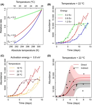
Figure 2. Example of temperature dependence of a rate for three different activation energies (Panel A) standardized to have the same value at 301.15 K (Huey and Kingsolver 2011). Panels B and C show the effect of activation energy (panel B) and temperature (panel C) on time series originated by the BDP 1 with parameters scaled using equation 2. The simulated time series all have an initial condition of 100 individuals are sampled everyday for 15 days
(TIMESAMP=15) and are subjected to demographic noise and sampling error (FRACSAMP=0.01). The continuous lines show the deterministic solution 13. Panel D shows real time series data (black dots) for 3 replicates ofParamecium caudatum
series recording the exact times of individual birth and death events. To make simulated data more representative of experimental data, we then sampled population size at discrete times as if only a fraction of the population had been sampled and counted (examples are shown in Fig. 2). To simulate sampling, we assumed that the num-bers measured were drawn from a Poisson distribution centered on the expected number of individuals contained in a sample from the population, where the sample size FRACSAMP is the fraction of the habitat searched. We do not include an additional source of error from the imperfect ability of observers to count all individuals in a sample; thus, demographic stochasticity and sampling error associated with the fraction of the habitat searched (FRACSAMP) are the only two sources of stochasticity in our simulated experimental data.
We chose parameter values for equations 1 and 2 that lead to similar simulated population dynamics to those observed in laboratory experiments (see Fig. 2) and that are consistent with previously published values (Savage et al. 2004). We set the reference temperature T0= 28°C and scaled the other population parameters relative to their probabilities at that temperature: h1(T0)= 1.5 day1, h2ð Þ ¼T0 1, h3(T0) =0.5 day1. The popula-tion size at which the probability of births is zero, N, was fixed throughout this study to N =15,000 individuals. The importance of this value is detailed in the discussion and here was chosen in order to represent a typical labo-ratory experiment with a microcosm of 10 mL.
These choices lead to a maximum population growth rate of r(T0)=1 day1and a minimum carrying capacity ofK(T0) =10,000 individuals. All simulations began with an initial population size of n0=100 individuals and lasted 15 days. We simulated equations 1 and 2 under 81 different sets of experimental conditions, representing the range of experimental strategies likely to be considered when conducting laboratory experiments to estimate acti-vation energy. These 81 experiments arise from a fully factorial experimental design in which four factors are varied, with three different values each. We varied • The number of different temperatures considered,
TEMPSAMP. We generated time series at 11 different temperatures from 18 to 28°C in steps of 1°C but var-ied the numbers of different temperatures used in the estimation of activation energy: either using all 11 tem-peratures, using only six different temperatures (from 18 to 28°C in steps of 2°C), or using just three different temperatures (18, 23 and 28°C). Those temperature gradients were chosen in order to capture the tempera-ture range where we expect the Arrhenius law 2 to be valid. Note that if a wider range of temperatures were to be investigated, then the rates may start to decrease
at higher temperatures, requiring fitting of a hump-shaped function rather than the Arrhenius equation (Corkrey et al. 2012; Krenek et al. 2012).
• The number of replicate experiments at each tempera-ture and activation energy, REPS. We considered one, three, or five replicates at each temperature. While esti-mation using one replicate per temperature is possible, from three to five are typically used in experiments where population time series are recorded (Leary and Petchey 2009; Krenek et al. 2011).
• The number of samples taken during an experiment, TIMESAMP. We considered once every three days (TIMESAMP = 5), twice every three days (TIMES-AMP = 10), or once a day (TIMES(TIMES-AMP = 15) over the course of each 15 days experiment. Fifteen days were sufficient to capture both the growth phase and the equilibrium phase (carrying capacity) of the population dynamics.
• The fraction of habitat sampled, FRACSAMP. We con-sidered 1%, 0.5%, and 0.1% of the entire habitat (FRACSAMP = 0.01, 0.005 and 0.001), reproducing the typical search effort of experiments (De Valpine and Hastings 2002; Dennis et al. 2006).
For each experimental design, we then estimate activa-tion energy using different methods.
Parameter inference
To conduct parameter inference, we need a mathematical function defining the probability of a set of parameters given the data, that is, the likelihood function. We com-pared different methods for inferring activation energy (summarized in Table 1) using five different likelihood functions (for details on the derivation of the likelihood functions see section “Likelihoods and inference” in Sup-porting information). The model underpinning methods M1 and M2 is the solution of equation 3, that is, the likeli-hood function is parameterized using only the mean popu-lation abundance overtime, assuming that the dynamics are deterministic. The second model (underpinning methods M3–M6) assumes that the dynamics are demographically stochastic but that there is no sampling error; the corre-spondent likelihood function is parameterized using both the mean and the variance of population abundance (see section “Details on the formulation of the stochastic model” in Supporting information and Ross et al. 2009 for the diffusion approximation used in the derivation of the population variance). In methods M7–M8, we add to the likelihood function of methods M3–M6 a correction taking into account for the sampling error.
indirectly, that is, population growth rates (r) or carrying capacities (K) are inferred at different temperatures. Acti-vation energy is then deduced from the relationship between these parameters and the inverse energy 1/kBT (see Fig. 2B) given by
logðK Tð Þ=r Tð ÞÞ ¼C1þ2EA 1
kBT; (6)
logðr Tð ÞÞ ¼C2EA 1
kBT; (7)
where C1 =log(N/h10/h20)2EAkB/T0 and C2¼log
ðh10h30Þ þEAkB=T0 are two temperature-independent constants. Activation energy is the slope of these relation-ships, derived using standard linear regression between the logarithm of the parameters of the logistic equation and the inverse temperature (Schoolfield et al. 1981; see Fig. 2B), as it has been extensively performed in previous studies (Schoolfield et al. 1981; Gillooly et al. 2001, 2002; Savage et al. 2004).
The other approach we take is to infer activation energy directly. Method M9 is a generalization of meth-ods M5–M6, and its likelihood is obtained by summing the likelihood underpinning methods M5–M6 over all observed temperatures. Similarly, method M10 is a gener-alization of methods M7–M8 and takes into account the sampling error. The likelihood of method M10 is obtained by summing the likelihoods of models M7–M8 over all observed temperatures (see section “Likelihoods and inference” for more details on the direct methods). The indirect methods used to infer activation energy are
characterized by the choice of one parameter (growth rate or carrying capacity) whose temperature dependence (relations 6 and 7) provides an estimate of activation energy. Direct methods, on the other hand, provide an estimate of activation energy from the global temperature dependency of all the parameters of model 1.
For each inference algorithm and experiment, we mea-sured the relative error (R) and precision (P) of the esti-mate given by
R¼EAmðEAÞ EA ;P¼
seðEAÞ
EA ; (8)
where EA is the real value of activation energy used to produce the simulated data, m(EA) is the mean of the estimate, andse(EA) is the standard error of the estimate. The accuracy of the estimates of activation energy is given by the inverse of the relative error R. When performing MLE, all the distributions of the parameters were assumed; Gaussian and the standard deviation were auto-matically inferred, while, when performing MCMC, we always checked the shape of the distribution to be a Gaussian, especially when performing the linear regres-sions 6 and 7 in the indirect models. Note that an increase in precision and accuracy corresponds to a decrease in the percentage given; in other words, high accuracy and precision correspond with low values of R andP.
[image:6.595.58.529.82.214.2]We then applied classification and regression tree analysis (CART) (Ripley 2007) to the absolute value of the relative error of the estimates of activation energy (the response variable) for each of the methods in
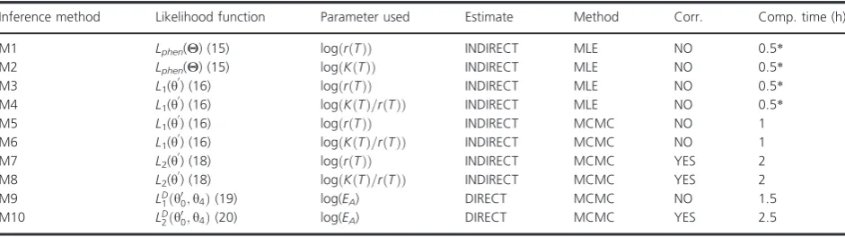
Table 1. Methods to infer activation energy.
Inference method Likelihood function Parameter used Estimate Method Corr. Comp. time (h)
M1 Lphen(Θ) (15) logðr Tð ÞÞ INDIRECT MLE NO 0.5*
M2 Lphen(Θ) (15) logðK Tð ÞÞ INDIRECT MLE NO 0.5*
M3 L1(h
0
) (16) logðr Tð ÞÞ INDIRECT MLE NO 0.5*
M4 L1(h
0
) (16) logðKðTÞ=r Tð ÞÞ INDIRECT MLE NO 0.5*
M5 L1(h
0
) (16) logðr Tð ÞÞ INDIRECT MCMC NO 1
M6 L1(h
0
) (16) logðKðTÞ=r Tð ÞÞ INDIRECT MCMC NO 1
M7 L2(h
0
) (18) logðr Tð ÞÞ INDIRECT MCMC YES 2
M8 L2(h
0
) (18) logðKðTÞ=r Tð ÞÞ INDIRECT MCMC YES 2
M9 LD
1ðh00;h4Þ(19) log(EA) DIRECT MCMC NO 1.5
M10 LD
2ðh00;h4Þ(20) log(EA) DIRECT MCMC YES 2.5
Table 1, in order to assess the relative importance of dif-ferent experimental factors (the explanatory variables) and their interaction (see Fig. 3). A regression tree is con-structed by repeated splits of the data into mutually exclusive groups. Each split is defined by values less than some chosen value of one of the experimental factors. At each split, the data are partitioned into two groups as homogenous as possible. Each group is distinguished by the mean of the absolute value of the relative error of the estimate of activation energy and the values of the experi-mental factors that define it (De’ath and Fabricius 2000; Ripley 2007). Splits are chosen in order to minimize the sum of squared error between the observation and the mean in each node of the tree. The splitting procedure is then applied to each group separately partitioning the response into homogeneous groups and keeping the tree sensibly small. Appropriate tree size is determined setting a threshold in the reduction in homogeneity measure
(De’ath and Fabricius 2000). Regression trees are a pow-erful tool for their capacity of interactive exploration and description of different subsets of the data and are often used instead of more classic linear model analysis (De’ath and Fabricius 2000).
Case study
As a case study, we present data from a microcosm exper-iment (Leary and Petchey 2009) in which time series of abundance were collected along a gradient of six different temperatures between 18 and 28°C, where there were three replicates and TEMPSAMP= 6 (please see Leary and Petchey 2009 for supplementary detail). In this case study, the fraction of habitat searched (FRACSAMP) and the frequency of sampling (TIMESAMP) were variable, the latter depending on the temperature and the former depending on the observed density; this was accounted
| FRACSAMP <0.005 TEMPSAMP <6 REP <3 TIMESAMP <10 TIMESAMP <10 REP <3 TEMPSAMP <6 REP <3 TIMESAMP <10 33 30 16 19 17 9 27 13 7 5 33 % 30 % 16 % 19 % 17 % 9 % 27 % 13 % 7 % 5 % | FRACSAMP <0.005 TIMESAMP <10 TEMPSAMP <6 REP <5 REP <3 REP <3 TEMPSAMP <6 37 17 18 20 9 18 9 6 37 % 17 % 18 % 20 % 9 % 18 % 9 % 6 % | FRACSAMP <0.005 REP <3 TIMESAMP <10 TEMPSAMP <6 TEMPSAMP <6 REP <3 60 35 34 20 13 12 6 60 % 35 % 34 % 20 % 13 % 12 % 6 % | FRACSAMP <0.005 TEMPSAMP <6 REP <3 32 21 17 10 32 % 21 % 17 % 10 % | FRACSAMP <0.005 TEMPSAMP <6 REP <5 TIMESAMP <15 41 87 37 32 13 41 % 87 % 37 % 32 % 13 % | REP <3 FRACSAMP <0.005 TEMPSAMP <6 TIMESAMP <10 368 89 54 44 30 368 % 89 % 54 % 44 % 30 %
(F) ( M 10 )
(E) ( M 9 )
(D) ( M 7 )
(C) ( M 5 )
(B) ( M 3 )
(A) ( M 1 )
for in the likelihood functions. We estimated the activa-tion energy of the protist species Paramecium caudatum in these microcosm experiments using methods M1, M2, M7, M8, and M10 (see Table 1 for definitions). Methods M7, M8, and M10 were used because we found them to be the most effective in estimating activation energy. Methods M1 and M2 (using the phenomenological likeli-hood 15, section “Likelilikeli-hoods and inference”) in Support-ing information were included to act as a comparison with the best performing methods because we wanted to investigate how important their lack of accuracy and pre-cision could be when estimating activation energy (see Fig. S2). We also found that real data do not strictly obey to the theory presented in (Savage et al. 2004) for carry-ing capacity (see Fig. 6B); for this reason, while uscarry-ing model M10, we implemented a likelihood with two differ-ent activation energies, one for growth rate (EA,r) and one for carrying capacity (EA,K).
Results
Activation energy was estimated with a wide range of accuracies across the different experimental conditions and inference methods considered, varying from high accuracy (relative error estimates being within <5% of the mean value on average) to low accuracy (relative error estimates being >300% of the average; Fig. 3). The fraction of the habitat sampled, FRACSAMP, was the most important experimental factor influencing the accuracy of activation energy estimates, as revealed by FRACSAMP consistently being the first split in five of six CART analysis (Fig. 3). An exception was when using method M1 (Fig. 3A), the phenomenological likeli-hood (equation 15, section “Likelilikeli-hoods and inference”) in Supporting information for parameter inference, which in general, produced relatively inaccurate esti-mates of activation energy. Therefore, for most methods, sampling >0.5% of the habitat leads to the biggest improvement in accuracy (decrease in relative error R) in the estimation of activation energy across all experi-mental factors. Also for the indirect methods which use carrying capacity as a parameter to infer activation energy (methods M2, M4, M6, and M8 in Table 1) the fraction of habitat searched is the most important exper-imental factor influencing the accuracy of activation energy estimates (see Fig. S1).
After FRACSAMP, there was no consistent ordering in the rank importance of the other experimental conditions across the different inference methods (Fig. 3). The num-ber of different temperatures used along a temperature gradient and the number of replicates per experiment were both used for the second split in the classification trees, depending on the inference method used. For the
number of replicates, accuracy was significantly lower for experiments with only one replicate than for those with more than one replicate. For example, when the fraction of habitat searched is >0.005, having at least three repli-cates instead of only one increases the accuracy of the estimates of activation energy from 16% to 10% error for method M5, from 12% to 6% error for method M7, and from 13% to 6% error for method M9 (Fig. 3A–D, respectively). For the number of temperatures, accuracy was significantly lower when just three temperatures were used than when more than three temperatures were used. The number of times in the 15 days period that samples were taken (TIMESAMP) appeared to have the smallest effect, although we expect this was because even the least frequent sampling still included low, medium, and high population densities in the time series. Replication also interacts with other factors such as the size of the temper-ature gradient (TEMPSAMP) to influence the accuracy of the estimates. For example, at low FRACSAMP, increasing the number of temperatures at which experiments are conducted will not increase the accuracy of estimates of activation energy when only one replicate is used per temperature when using indirect methods (Fig. 3D). However, having more temperatures will improve the estimate of activation energy when using a direct method (Fig. 3F).
Taking into account, the observation error in the infer-ence method increased the accuracy of estimates of acti-vation energy when inferring it indirectly for carrying capacity (mean relative error of method M6 of 45% vs. mean relative error of M8 is 36%) and growth rate (mean relative error of method M5 is 16% vs. mean relative error of M7 is 11%). However, it led to only a minor improvement when inferring activation energy directly (mean relative error of method M9 is 10.6% vs. mean rel-ative error of M10 is 10.3%). Estimates of activation energy are generally more accurate when estimated using MCMC parameter inference than using MLE, although sampling a larger fraction of the microcosm can clearly be used to compensate for this (see Fig. 4). Among the indirect MCMC methods, more accurate estimates of acti-vation energy were obtained using the inferred growth rate rather than carrying capacity, and accounting for observational error improved these estimates further. These improvements were made with the inevitable cost of computational time (Table 1).
An exception is direct inference method M9 in which appears to consistently underpredict activation energy at low sampling intensities, which appears to be corrected by taking into account sampling error in method M10. Given the inferior performance of the MLE methods and the dominance of FRACSAMP, we only describe how the precision of estimates is affected by FRACSAMP for the MCMC methods. The most precise estimates of activation energy tend to be obtained using either the direct meth-ods or the indirect methmeth-ods on growth rate only with sampling error correction (Fig. 5 M7, M9, M10; the results illustrated in this figure are representative of what we observed for other sets of experimental conditions). In general, the most precise estimates were obtained using the direct methods (M9 and M10) which combine infor-mation on both growth rates and carrying capacities. Implementing the sampling error correction also tends to increase the precision of the estimated activation energies (Fig. 5). Interestingly, direct methods (M9 and M10) are clearly more sensitive to changes in the experimental con-ditions, as shown by the largest number of statistically significant branches in the regression trees (Fig. 3E and F).
When used on real time series data, inferred population growth rate is linearly related to the inverse of tempera-ture, with a negative slope given by the activation energy, as predicted by metabolic theory (Savage et al. 2004; Fig. 6A). In contrast, the temperature dependence of car-rying capacity does not follow the theory (which predicts a positive relationship, Savage et al. 2004), showing no clear directional relationship with temperature (Fig. 6B). For the best performing methods in our simulation experiments (methods M7, M8, and M10), the direct and indirect methods produce different estimates of activation energy. The estimate for population growth rate from
−3
−2
−1
0
1
2
3
FRACSAMP 0.001
−3
−2
−1
0
1
2
3
FRACSAMP 0.005
M1 M2 M3 M4 M5 M6 M7 M8 M9 M10
−3
−2
−1
0
1
2
3
Method
[image:9.595.67.293.70.384.2]FRACSAMP 0.01
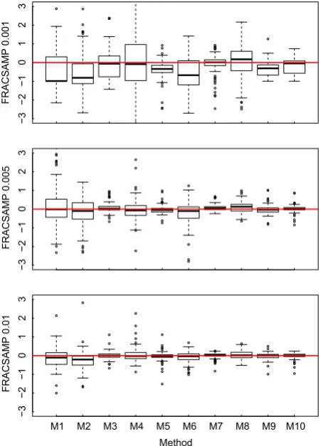
Figure 4. The variation in the relative error of each model indicated in Table 1 for different FRACSAMP, for experiments with one replicate, for each activation energies used in simulated data (EA=0.2–1.2 eV) for all values of TIMESAMP (5,10,15) and TEMPSAMP (3,6,11). The y axis displays percentage values of relative error. The black lines indicate the medians, and the boxes demarcate the 25–75% intervals. The whiskers extend up to one and a half times the interquartile range. The red line shows the maximum precision (i.e., estimated value=true value).
M5 M6 M7 M8 M9 M10
−0.5
0.0
0
.5
1.0
0.001 FRACSAMP
Method
M5 M6 M7 M8 M9 M10
−0.5
0.0
0
.5
1.0
0.005 FRACSAMP
Method
M5 M6 M7 M8 M9 M10
−0.5
0.0
0.5
1.0
0.01 FRACSAMP
Method
[image:9.595.66.540.510.662.2]the direct method is slightly lower (EA= 0.8 eV) than the estimate obtained indirectly (EA=0.9 eV). For the temperature range we considered, this difference leads to the largest contrast between predicted growth rates at T= 28°C, where the difference is roughly 1 day1. Differ-ences in the the mean estimates of activation energy of carrying capacity using direct and indirect methods do not lead to different predicted mean carrying capacities at different temperatures (largely because the estimated acti-vation energy is close to zero). However, the precision of
those predictions do contrast; for example, at T= 28°C, the standard deviation of the predicted carrying capacity is approximately 1000 individuals when using the direct method and is approximately 4500 individuals when using the indirect methods. An example of the different estimates obtained with direct and indirect methods at a given temperature (T= 22°C) is shown in Figure 2D. The activation energy of growth rate measured with the direct method is smaller than the one obtained with indi-rect methods and has a smaller error.
Applying the phenomenological methods leads to nota-ble differences in the accuracy of the estimates of activa-tion energy for the microcosm experiments. Using indirect method M1 (phenomenological) to estimate acti-vation energy leads to an estimate, that is, 0.2 eV lower than that generated by indirect method M7 (0.7 eV com-pared to 0.9 eV, respectively; Fig. S2A). This difference translates to a difference in predicted growth rate at T=28°C of 1.2 day1. A similar difference is observed when estimating the activation energy of carrying capac-ity: indirect method M2 (phenomenological) gives an estimate, that is, 0.2 eV higher than that generated by indirect method M8 (0.03 eV compared to 0.2 eV, respectively; Fig. S2B). In this example, this could lead to a qualitatively different conclusion about whether carrying capacity is related to temperature, with the phenomeno-logical method implying a positive relationship, whereas method M8 implies no relationship.
Discussion
Our results revealed how experimental factors and param-eter inference methods interact to influence the accuracy with which activation energy can be inferred. We found that the fraction of habitat searched is the most impor-tant factor in determining the accuracy of the estimates of activation energy. We also provided a list of inference methods from the least to the most accurate, for a set of experimental designs (see Fig. 4), including a classic phe-nomenological likelihood (Pascual and Kareiva 1996) where no information about demographic stochasticity was included, likelihoods that accounted for demographic stochasticity (Ross et al. 2006), and likelihoods that accounted for demographic stochasticity and sampling error (Ross et al. 2009). Inference methods that included the different sources of stochasticity improved the preci-sion and the accuracy of the estimates of activation energy of at least one order of magnitude, for a given experimental design, especially when the fraction of habi-tat searched was small. The largest improvement in the accuracy of the estimates was obtained using a diffusion approximation (Ross et al. 2006, 2009) for continuous time stochastic processes. The use of such approximation
38.6 39.0 39.4 39.8
0.0
0
.5
1.0
1
.5
2.0
Inverse energy (1/Ev)
Log (r)
18 20 22 24 26 28
Temperature (ºC)
EACT= 0.9 ± 0.07 Ev EACT= 0.8 ± 0.07 Ev
38.6 39.0 39.4 39.8
9.0
10.0
11.0
1
2.0
Inverse energy (1/Ev)
Log (K)
18 20 22 24 26 28 Temperature (ºC)
EACT = 0.03 ± 0.2 Ev EACT = 0.14 ± 0.06 Ev (A)
[image:10.595.86.258.67.432.2](B)
enabled us to disentangle different sources of noise (demographic and sampling) and could be extended to more complex models. Another key improvement to the inference was fitting (directly) to all available data simul-taneously. Moreover, taking into account the sampling error correction in direct methods, where the information of both temperature dependencies of growth rate and car-rying capacity is taken into account, slightly improved the estimate of activation energy. Application of these simula-tion-based findings to real data suggests that although this direct method is more accurate, prior use of the indirect method is useful to reveal the functional form of the tem-perature dependency.
Comparison of the indirect and direct methods of inference revealed the unique strengths of each approach. Indirect methods are useful to identify the strengths and weaknesses of the different models describing single tem-perature time series. Once a suitable functional form is implemented, the temperature dependence of ecological parameters can be better inferred using direct methods; yet direct methods could be misleading if applied with-out having a clear understanding of the with-outcome of the indirect methods. For example, in our study, we based our simulations on a specific exponential function (Arrhenius law) scaled with a single parameter (activation energy). Different functional forms (such as hump-shaped functions) would have required a different imple-mentation into direct methods. Similar approaches have been used in other modeling frameworks (Grimm et al. 2005; Smith et al. 2013) where parameter borrowing between different experiments is used to inform the glo-bal parameterization of the model (McInerny and Purves 2011; Sibly et al. 2013; Smith et al. 2013). The direct approach could be further generalized in more complex models such as food web models (Petchey et al. 2010) or stage-structured models (Ananthasubramaniam et al. 2011). When assessing the performance of different mod-els against data, direct and indirect methods should be combined.
When using direct methods on time series data for Paramecium caudatum, we found that the estimates of growth rate at each temperature were affected by the estimates of carrying capacity, thus giving “neighborly advice” (McInerny and Purves 2011) on the temperature dependence of growth rate. The difference in estimation between direct and indirect methods led to large differ-ences in predicted population dynamics (Fig. 2D). The thermal performance curves of Paramecium caudatum have been assessed only using indirect methods (using growth rate as reference parameter; Krenek et al. 2011), and several models have been proposed to capture the temperature dependence of microbial growth (Huang et al. 2011; Krenek et al. 2011). We provide a
frame-work to test further the thermal performance of micro-bial organisms, combining the information of carrying capacity with the information on growth rate. Our methods could be used to compare different thermal performance curves in microbial experiments (Angiletta 2006) and be further tested with different processes such as feeding rates (Rall et al. 2009; Englund et al. 2011; Fussmann et al. 2014) and with different environmental variables such as nutrient concentration (Weisse et al. 2002).
The use of stochastic models such as continuous birth and death processes (McKane and Newman 2004; Black and McKane 2012) provides a probabilistic framework to derive inference schemes from (Ross et al. 2006, 2009) and provides insight into the determinants of population dynamics (Black and McKane 2012). Despite the lack of a mathematical expression for the probability distribution of the populations in our study, the use of approxima-tions, such as the diffusion one, provided an analytical expression for the first two moments of the population probability distribution (Ross et al. 2009; Ross 2012). Extending stochastic models to different systems with more than one species is analytically daunting, but numerically feasible. The mechanistic understanding of more complex multispecies models is then limited by their mathematical intractability. When it is not possible to obtain analytical expressions for population probability distributions, the Bayesian framework can be still used with numerical techniques such as particle filters (Ionides 2003; Ionides et al. 2006) or approximate Bayesian com-putation (Beaumont 2010). Those methods simulate directly, with a given precision, the likelihood of the model at each iteration of the Markov chain (Hartig et al. 2011). Markov chain Monte Carlo methods are more computationally demanding than classic maximum likeli-hood estimation, especially when implementing state space models; however, they give a more complete esti-mation of the probability distribution of the parameters of the model and of their correlation, especially when the distribution of those parameters is not Gaussian.
to differences in demographic noise which could influence the precision with which we can estimate activation energy. However, the temperature dependence of growth rate and carrying capacity is not dependent on N in our simulation experiments, and so we expect that, given an adequate amount of sampling and a sufficiently large temperature range, our conclusions about the effects of likelihood methods and experimental design on estimates of activation energy will be insensitive to our choice ofN. Again for simplicity, we assumed that density dependence only influences the probability of births while in reality, it commonly influences the probability of both. In section “Details on the formulation of the stochastic model”, in Supporting information we give the formulations for the more general birth and death processes in which both birth and death rates depend on N. When combined, these lead to more free parameters, but identical formula-tions for the temperature dependence of population growth rate and carrying capacity; thus, our results would be unaffected.
Our methods could improve the development of the ecological theory aimed at understanding the temperature dependence of population rates (Brown et al. 2004; Amarasekare and Savage 2012) or inform debates about the precise value of activation energy (Glazier 2006). The use of classic indirect methods can be used as a first step in identifying reasonable functional forms for the temper-ature dependence of population parameters, as biologists have extensively performed for a variety of taxa (Gillooly et al. 2001; Savage et al. 2004; Amarasekare and Sifuentes 2012). Different models associated with different func-tional forms of the rate temperature relations have now been proposed (Brown et al. 2004; Knies and Kingsolver 2010; Amarasekare and Savage 2012), and those models, arising from the combination of data and theory, can be further tested using the direct estimation methods we describe here.
One of the remaining conundrums in population and community ecology is about predictive ability. Studies have shown that uncertainty in parameter estimates can preclude predictions of even the direction (increase or decrease) of the effects of a perturbation (Yodzis 1988; Wells et al. 2014) but also that more accurate estimates will provide better predictions (Novak et al. 2011). Our findings support the idea that considerable potential for improved predictive ability lies in improving inference methods, including using quite complex mathematics and fitting algorithms, as well as continuing to use appropri-ate experimental designs and sampling schemes. The resulting increases in accuracy are likely to be very impor-tant, given the documented high sensitivity of model pre-dictions to variation in parameter values.
Acknowledgments
The project is funded by Microsoft Research and The University of Zurich.€
Conflict of Interest
None declared.
References
*Allen, L. J. S., and E. J. Allen. 2003. A comparison of three different stochastic population models with regard to persistence time. Theor. Popul. Biol. 64:439–449.
Allen, A. P., J. F. Gillooly, and J. H. Brown. 2005. Linking the global carbon cycle to individual metabolism. Funct. Ecol. 19:202–213.
Amarasekare, P., and V. M. Savage. 2012. Elucidating the temperature dependence of fitness. Am. Nat. 179:178– 191.
Amarasekare, P., and R. Sifuentes. 2012. Elucidating the temperature response of survivorship in insects. Funct. Ecol. 26:959–968.
Ananthasubramaniam, B., R. M. Nisbet, W. A. Nelson, E. McCauley, and W. S. C. Gurney. 2011. Stochastic growth reduces population fluctuations in Daphnia-algal systems. Ecology 92:362–372.
Angiletta, M. J. Jr. 2006. Estimating and comparing thermal performance curves. J. Therm. Biol. 31:541–545.
Arrhenius, S. 1889.Uber die reaktionsgeschwindigkeit bei der€ inversion von rohrzucker durch s€auren. Z. Phys. Chem. 4:226–248.
Beaumont, M. A. 2010. Approximate Bayesian Computation in evolution and ecology. Annu. Rev. Ecol. Evol. Syst. 41:379– 406.
Beveridge, O. S., O. L. Petchey, and S. Humphries. 2010. Direct and indirect effects of temperature on the population dynamics and ecosystem functioning of aquatic microbial ecosystems. J. Anim. Ecol. 79:1324–1331.
Black, A. J., and A. J. McKane. 2012. Stochastic formulation of ecological models and their applications. Trends Ecol. Evol. 27:337–345.
*Bolker, B. 2013. Bbmle: Tools for general maximum likelihood estimation. R package version 1.0-13.
Brown, J. H., J. F. Gillooly, A. P. Allen, V. M. Savage, and G. B. West. 2004. Toward a Metabolic Theory of Ecology. Ecology, 85:1771–1789.
*Cappe, O., E. Moulines, and T. Ryden. 2005. Inference in hidden Markov models. Springer Series in Statistics XVIII. Springer, New York.
*Chib, S., and E. Greenberg. 1995. Understanding the Metropolis-Hasting algorithm. Am. Stat. 49:327–335. Corkrey, R., J. Olley, D. Ratkowsky, T. McMeekin, T. Ross
Governing Biological Growth Rates. PLoS One 7(2): e32003. doi: 10.1371/journal.pone.0032003.
De Valpine, P., and A. Hastings. 2002. Fitting population models incorporating process noise and observation error. Ecol. Monogr. 72:57–76.
De’ath, G., and K. E. Fabricius. 2000. Classification and regression trees: a powerful yet simple technique for ecological data analysis. Ecology 81:3178–3192. Dell, A. I., S. Pawar, and V. M. Savage. 2010. Systematic
variation in the temperature dependence of physiological and ecological traits. Proc. Natl Acad. Sci. USA 108:10591–10596. Dell, A. I., S. Pawar, and V. M. Savage. 2014. Temperature
dependence of trophic interactions are driven by asymmetry of species responses and foraging strategy. J. Anim. Ecol. 83:70–84.
Dennis, B., and J. M. Ponciano. 2014. Density-dependent-state space model for population-abundance with unequal time intervals. Ecology 95:2069–2076.
Dennis, B., J. M. Ponciano, S. R. Lele, M. L. Taper, and D. F. Staples. 2006. Estimating density dependence, process noise, and observation error. Ecol. Monogr. 76:323–341.
Deutsch, C. A., J. J. Tewksbury, R. B. Huey, K. S. Sheldon, C. K. Ghalambor, D. C. Haak, et al. 2008. Impacts of climate warming on terrestrial ectotherms across latitude. Proc. Natl Acad. Sci. USA 105:6668–6672.
Ebenman, B., R. Law, and C. Borrvall. 2004. Community viability analysis: the response of ecological communities to species loss. Ecology 85:2591–2600.
Englund, G., G. Ohlund, C. L. Hein, and S. Diehl. 2011. Temperature dependence of the functional response. Ecol. Lett. 14:914–921.
Ernest, S. K. M., B. J. Enquist, J. H. Brown, E. L. Charnov, J. F. Gillooly, V. M. Savage, et al. 2003. Thermodynamic and metabolic effects on the scaling of production and population energy use. Ecol. Lett. 6:990–995.
*Filzbach, Microsoft Research Cambridge. 2013. Available via http://research.microsoft.com/en-us/um/cambridge/groups/ science/tools/filzbach/filzbach.htm
Fussmann, K. E., F. Schwarzm€uller, U. Brose, A. Jousset, and B. C. Rall. 2014. Ecological stability in response to warming. Nat. Clim. Chang. 4:206–210.
Gardinier, C. 2009. Stochastic methods: a handbook for the natural and social sciences. Springer, Berlin.
Gillespie, D. T. 1976. A general method for numerically simulating the stochastic time evolution of coupled chemical reactions. J. Comput. Phys. 22:403–434.
*Gillespie, D. T. 1977. Exact stochastic simulation of coupled chemical reactions. J. Phys. Chem. 81:2340–2361.
Gillooly, J. F., J. H. Brown, G. B. West, V. M. Savage, and E. L. Charnov. 2001. Effects of size and temperature on metabolic rate. Science 293:2248–2251.
Gillooly, J. F., E. L. Charnov, G. B. West, V. M. Savage, and J. H. Brown. 2002. Effects of size and temperature on developmental time. Nature 417:70–73.
Glazier, D. S. 2006. The 3/4-power law is not universal: evolution of isometric, ontogenetic metabolic scaling in pelagic animals. Bioscience 56:325–332.
Grimm, V., E. Revilla, U. Berger, F. Jeltsch, W. M. Mooij, S. F. Railsback, et al. 2005. Pattern-oriented modeling of agent-based complex systems: lessons from ecology. Science 310:987–991.
Hall, A. S. C., J. A. Stanford, and F. R. Hauer. 1992. The distribution of abundance of organisms as a consequence of energy balances along multiple environmental gradients. Oikos 65:377–390.
Hartig, F., J. M. Calabrese, B. Reineking, T. Wiegand, and A. Huth. 2011. Statistical inference for stochastic simulation models - theory and application. Ecol. Lett. 14:86–827. Hilborn, R. 1997. The ecological detective: confronting models
with data. Princeton Univ. Press, Princeton, New Jersey. Huang, L., A. Hwang, and J. Phillips. 2011. Effect of
temperature on microbial growth rate-mathematical analysis: the Arrhenius and Eyring-Polany corrections. J. Food Sci. 76:553–560.
Huey, R. B., and J. G. Kingsolver. 2011. Variation in universal dependence of biological rates. Proc. Natl Acad. Sci. USA 108:10377–10378.
Ionides, E. L. 2003. Inference and filtering for partially observed diffusion processes via sequential Monte Carlo. Department of Statistics Technical Report, The University of Michigan, Ann Arbor.
Ionides, E. L., C. Breto, and A. A. King. 2006. Inference for nonlinear dynamical systems. Proc. Natl Acad. Sci. USA 103:18438–18443.
Irlich, U. M., J. S. Terblanche, T. M. Blackburn, and S. L. Chown. 2009. Insect rate-temperature relationships: environmental variation and the metabolic theory of ecology. Am. Nat. 174:819–835.
Ives, A. R. 1995. Predicting the response of populations to environmental change. Ecology 76:926–941.
Jang, L., and P. J. Morin. 2004. Temperature-dependent interactions explain unexpected responses to environmental warming in communities of competitors. J. Anim. Ecol. 73:569–576.
*Kirkpatrick, S., C. D. Gelatt, and M. P. Vecchi. 1983. Optimization by simulated annealing. Science 220:671–680. Knape, J., and P. De Valpine. 2012. Fitting complex
population models by combining particle filters with Markov chain Monte Carlo. Ecology 93:256–263. Knies, L., and J. G. Kingsolver. 2010. Erroneus Arrhenius:
modified Arrhenius model best explains the temperature dependence of ectotherm fitness. Am. Nat. 176:227–233. Krenek, S., T. U. Berendonk, and T. Petzoldt. 2011. Thermal
performance curves of Paramecium caudatum: a model selection approach. Eur. J. Protistol. 47:124–137. Krenek, S., T. Petzoldt, and T. U. Berendonk. 2012. Coping
caudatum. PLoS One, 7. Available via http://dx.doi.org/10. 1371/journal.pone.0030598
Leary, D. J., and O. L. Petchey. 2009. Testing a biological mechanism of the insurance hypothesis in experimental aquatic communities. J. Anim. Ecol. 78:1143–1151.
Leary, D. J., J. M. K. Rip, and O. L. Petchey. 2012. The impact of environmental variability and species composition on the stability of experimental microbial populations and communities. Oikos 121:327–336.
Malthus, T. 1798. An essay on the principle of population. J. Johnson, London.
McInerny, G. J., and D. W. Purves. 2011. Fine-scale environmental variation in species distribution modelling: regression dilution, latent variables and neighbourly advice. Methods Ecol. Evol. 2:248–257.
McKane, A. J., and T. J. Newman. 2004. Stochastic models in population biology and their deterministic analogs. Phys. Rev. E 70:1–19.
McKane, A. J., and T. J. Newman. 2005. Predator-prey cycles from resonant amplification of demographic stochasticity. Phys. Rev. Lett. 94:1–4.
Monod, J. 1942. Recherches sur la croissance des cultures bacteriennes. Hermann, Paris.
Montagnes, D. J. S., and D. J. Franklin. 2001. Effect of temperature on diatom volume, growth rate, and carbon and nitrogen content: reconsidering some paradigms. Limnol. Oceanogr. 46:2008–2018.
Montagnes, D. J. S., S. A. Kimmance, G. Tsounis, and J. C. Gumbs. 2001. Combined effect of temperature and food concentration on the grazing rate of the rotifer Brachionus plicatilis. Mar. Biol. 139:975–979.
Nasell, I. 2001. Extinction and quasi-stationarity in the Verhulst logistic model. J. Theor. Biol. 211:11–27. Novak, M., J. T. Wootton, D. F. Doak, M. Emmerson, J. A.
Estes, and M. T. Tinker. 2011. Predicting community responses to perturbations in the face of imperfect knowledge and network complexity. Ecology 92:836–846. O’Connor, M. I., B. Gilbert, and C. J. Brown. 2011.
Theoretical predictions for how temperature affects the dynamics of interacting herbivores and plants. Am. Nat. 178:626–638.
Pascual, M. A., and P. Kareiva. 1996. Predicting the outcome of competition using experimental data: Maximum Likelihood and Bayesian approaches. Ecology 77:337–349. Petchey, O. L., U. Brose, and B. C. Rall. 2010. Predicting the
effects of temperature on food web connectance. Philos. Trans. R. Soc. Lond. B Biol. Sci. 365:2081–2091.
Price, P. B., and T. Sowers. 2004. Temperature dependence of metabolic rates for microbial growth, maintenance, and survival. Proc. Natl Acad. Sci. USA 101:4631–4636. Rall, B. C., O. Vucic-Pestic, R. B. Ehnes, M. Emmerson, and
U. Brose. 2009. Temperature, predator-prey interaction strength and population stability. Glob. Change Biol. 16:2145–2157.
Ripley, B. 2007. Tree: classification and regression trees. R package version 1.0-26.
Ross, J. V. 2012. On parameter estimation in population models III: time-inhomogeneous processes and observation error. Theor. Popul. Biol. 82:1–17.
Ross, J. V., T. Taimre, and P. K. Pollett. 2006. On parameter estimation in population models. Theor. Popul. Biol. 70:498–510.
Ross, J. V., D. E. Pagendam, and P. K. Pollett. 2009. On parameter estimation in population models II:
multi-dimensional processes and transient dynamics. Theor. Popul. Biol. 75:123–132.
Savage, V. M., J. F. Gillooly, J. H. Brown, G. B. West, and E. L. Charnov. 2004. Effects of body size and temperature on population growth. Am. Nat. 3:429–441.
Schoolfield, R. M., P. J. H. Sharpe, and C. E. Magnuson. 1981. Nonlinear regression of biological temperature-dependent rate models based on absolute reaction-rate theory. J. Theor. Biol. 88:719–731.
Sibly, R. M., V. Grimm, B. T. Martin, A. S. A. Johnston, K. Kulakowska, C. J. Topping, et al. 2013. Representing the acquisition and use of energy by individuals in agent-based models of animal populations. Methods Ecol. Evol. 4:151– 161.
Smith, M. J., D. W. Purves, M. C. Vanderwel, V. Lyutsarev, and S. Emmott. 2013. The climate dependence of the terrestrial carbon cycle, including parameter and structural uncertainties. Biogeosciences 10:583–606.
Thomas, C. D., A. Cameron, R. E. Green, M. Bakkenes, L. J. Beaumont, Y. C. Collingham, et al. 2004. Extinction risk from climate change. Nature 427:145–148.
Turchin, P. 2003. Complex population dynamics: a theoretical/ empirical synthesis. Princeton Univ. Press, Princeton, New Jersey.
Van’t Hoff, J. H. 1884. Etudes de dynamique chimique F. Muller & Co., Amsterdam.
Vasseur, D. A., and K. S. McCann. 2005. A mechanistic approach for modeling temperature-dependent consumer-resource dynamics. Am. Nat. 166:184–198. Vasseur, D. A., J. P. DeLong, B. Gilbert, H. S. Greig, C. D.
G. Harley, K. S. McKann, et al. 2014. Increased temperature variation poses a greater risk to species than climate warming. Proc. R. Soc. B Biol. Sci. 281:20132612.
Volkov, I., J. R. Banavar, S. P. Hubbell, and A. Maritan. 2003. Neutral theory and relative species abundance in ecology. Nature 424:1035–1037.
Weisse, T., and D. J. S. Montagnes. 1998. Effect of
temperature on inter- and intraspecific isolates of Urotricha (Prostomatida, Ciliophora). Aquat. Microb. Ecol. 15:285– 291.
the small freshwater ciliate Urotricha farcta. Limnol. Oceanogr. 47:1447–1455.
Wells, K., H. Feldhaar, and R. B. O’Hara. 2014. Population fluctuations affect inference in ecological networks of multi-species interactions. Oikos 123:589–598.
*Wilkinson, D. 2006. Stochastic modelling for systems biology. Chapman & Hall/CRC, London.
Yodzis, P. 1988. The Indeterminacy of Ecological Interactions as Perceived Through Perturbation Experiments. Ecology 69:508–515.
Yodzis, P., and S. Innes. 1992. Body size and
consumer-resource dynamics. Am. Nat. 139:1151–1175. Yvon-Durocher, G., J. M. Caffrey, A. Cescatti, M. Dossena,
P. Del Giorgio, J. M. Gasol, et al. 2012. Reconciling the temperature dependence of respiration across timescales and ecosystem types. Nature 487:472–476.
*References are cited in supporting information.
Supporting Information
Additional Supporting Information may be found in the online version of this article:
Data S1. Time series of the species Paramecium caudatum at different temperatures.
Figure S1. The results of the classification and regression tree (CART) analysis (Ripley 2007) of the relative error of the estimates of activation energy. The number at the leaves of the tree indicates the mean percentage value of
the relative error of the estimate (see expression 8) over all the simulated experiments, following partitioning of the data in the manor specified by the tree. The threshold above each node indicates the split criterion used to sepa-rate the data. To each tree is associate a bar chart show-ing the mean percentage value of each leaf. The four panels correspond to four of the models specified in Table 1: model M2 (panel A), M4 (panel B), M6 (panel C), and M8 (panel D).