Evolution of prolate molecular clouds at H
II
boundaries – I. Formation
of fragment-core structures
T. M. Kinnear,
1‹J. Miao,
1G. J. White
2,3and S. Goodwin
41Centre for Astrophysics and Planetary Science, School of Physical Sciences, University of Kent, Canterbury CT2 7NH, UK 2Department of Physics and Astronomy, The Open University, Milton Keynes MK7 6AA, UK
3Space Science and Technology Department, CCLRC Rutherford Appleton Laboratory, Oxfordshire OX11 0QX, UK 4Department of Physics and Astronomy, University of Sheffield, Sheffield S3 7RH, UK
Accepted 2014 July 21. Received 2014 July 21; in original form 2014 February 11
A B S T R A C T
The evolution of a prolate cloud at an HIIboundary is investigated using smoothed particle
hydrodynamics. The prolate molecular clouds in our investigation are set with their semi-major axis perpendicular to the radiative direction of a plane-parallel ionizing extreme ultraviolet (EUV) flux. Simulations on three high-mass prolate clouds reveal that EUV radiation can trigger distinctive high-density core formation embedded in a final linear structure. This contrasts with results of the previous work in which only an isotropic far-ultraviolet interstellar background flux was applied. A systematic investigation on a group of prolate clouds of equal mass but different initial densities and geometric shapes finds that the distribution of the cores over the final linear structure changes with the initial conditions of the prolate cloud and the strength of the EUV radiation flux. These highly condensed cores may either scatter over the full length of the final linear structure or form two groups of high-density cores at two foci, depending on the value of the ionizing radiation penetration depthdEUV, the ratio of the
physical ionizing radiation penetration depth to the minor axis of the cloud. Data analysis on the total mass of the high-density cores and the core formation time finds that the potential for EUV radiation triggered star formation efficiency is higher in prolate clouds with shallow ionization penetration depth and intermediate major-to-minor axial ratio, for the physical environments investigated. Finally, it is suggested that the various fragment-core structures observed at HIIboundaries may result from the interaction between ionizing radiation and
pre-existing prolate clouds of different initial geometrical and physical conditions.
Key words: hydrodynamics – radiative transfer – stars: formation – ISM: evolution – HII
regions – ISM: kinematics and dynamics.
1 I N T R O D U C T I O N
Newly formed massive stars emit intense UV radiation on to the surfaces of surrounding molecular clouds, ionizing and heating gas on their star-facing surfaces. The ionization heating ejects the ion-ized gas from the cloud to create a hot and diffuse HIIregion, whilst
at the same time drives a compressive wave towards the interior of the cloud to form condensed core(s), in which new star(s) could form. This is the so-called radiation-driven implosion (RDI) process (Bertoldi1989). Additionally, emission from the recombination of electrons with ions creates a bright rim at the edge of the molecular cloud on its star-facing side. The resultant cloud structure contain-ing a bright rim and condensed core is termed a bright-rimmed
E-mail:[email protected]
cloud (BRC), which has interested astronomers over the last two decades, and their study has been an important observational step in the development of models of triggered star formation (Elmegreen & Lada1977; McKee & Hollenbach1980; Sandford, Whitaker & Klein1982).
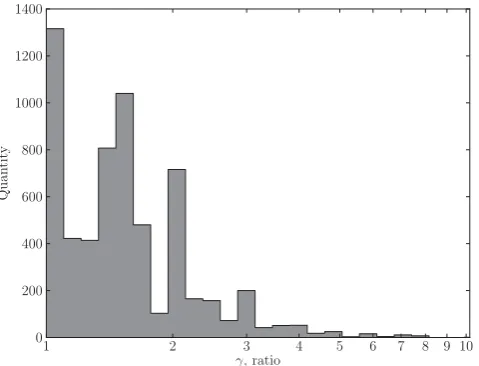
Figure 1. The distribution of molecular clumps over the semi-major to minor axial ratiosγ. Statistics based on the data in a survey for 6124 single molecular clumps (Rathborne et al.2009).
Bhatt2010; Chauhan et al.2011) and symmetrical BRC structures sandwiched between two HIIregions (Cohen, Staveley-Smith & Green2003; Ojha et al.2011).
Based on the RDI mechanism, current theoretical investigations have successfully revealed a possible physical process for the for-mation of BRCs having symmetrical morphologies (Bertoldi1989; Lefloch & Lazareff1994, 1995; Kessel-Deynet & Burkert2000, 2003; Esquivel & Raga2007; Miao et al.2006,2009; Gritschneder et al.2009; Bisbas et al.2011; Haworth & Harries2012). Although Miao et al. (2010) have studied the possibility for the formation of the IC59 structure (type M; Karr et al.2005), little attention has been paid to explore the RDI triggered star formation process in asymmetrical BRCs.
Most of the current RDI models adopt a spherical molecular cloud as the initial condition in simulations. However, recent obser-vations on a large sample of isolated molecular cores have revealed that spherically symmetric molecular cloud cores are the excep-tion rather than the rule (Myers et al.1991; Curry & Stahler2001; Jones, Basu & Dubinski2001; Rathborne et al.2009). Theoretical investigations have also found physical mechanisms which result in the formation of prolate clouds in general astrophysical envi-ronments (Tassis2007; Boss2009; Cai & Taam2010). Shown in Fig.1is the distribution of molecular clumps over the ratioγof the semi-major (a) to semi-minor (b) axis, resulted from a Galactic Ring Survey of 6124 objects, which gives a mean axial ratioγ = ab =1.6 (Rathborne et al.2009). It is worth noting that the data from which these ratios were calculated were determined using the full width at half-maximum of two axes in the observation. As such, clumps which are elongated but have their semi-major axis intercepting the observational plane by an angle are represented with a lowerγ
value than their actual ones. It can be expected that the ‘true’ ratios of these objects will be shifted to higherγ value range.
Therefore, the assumption of an initially spherical molecular cloud in theoretical modelling may be too simplistic for a complete view of the diverse structures found at HIIboundaries. Although
some previous work has investigated the collapse of a prolate cloud subject to an isotropic far-ultraviolet (FUV) radiation field (Nelson & Langer1997), the dynamical evolution of a prolate cloud at an HIIboundary has not yet been investigated. Therefore, we have
at-tempted to investigate this scenario with prolate molecular clouds of
various initial geometries and physical conditions. Our objective is to explore possible physical mechanisms for a variety of structures found at HIIboundaries but not yet well understood.
In this paper, we focus on the investigation of the evolution of a prolate cloud at an HIIboundary with its semi-major axis
per-pendicular to the ionizing radiation flux. In Section 2, we briefly describe the numerical codes used along with data processing, as well as the initial conditions of the prolate clouds adopted in our simulations. Our simulation results and discussions are presented in Section 3 and the conclusions are discussed in Section 4. Table1 describes all of the test series used in the paper, along with their purpose and the section(s) in which they are discussed.
2 T H E C O D E A N D I N I T I A L C O N D I T I O N S
2.1 The code
All of the simulations presented in this paper were performed us-ing an extended smoothed particle hydrodynamics (SPH) code II, which is based on the SPH code I by Nelson & Langer (1997). The latter was used to investigate the evolution of a molecular cloud in an isotropic interstellar background FUV radiation field. Code I was extended by including extreme ultraviolet (EUV) radiation transfer-ring into a molecular cloud and the consequent physical processes. Therefore, the recently refined code II contains the following com-ponents: (i) SPH solvers for the full set of standard hydrodynamic equations (including energy evolution equation); (ii) ray-tracing solver for the radiation transferring equations, which is based on the method of Kessel-Deynet & Burkert (2000); (iii) a numerical solver for a set of chemical reaction differential equations, which evolves the fractional abundances of the chemical species: CO, CI,
CII, HCO+, O, He+, OHx, CHx, H+3, M, M+ and free electrons
(Nelson & Langer1997). Further details of code II can be found in Miao et al. (2006). In the following, we present a brief summary of its main features.
In the hydrodynamic equation solver, each SPH particle is given an adaptive smoothing lengthh; therefore, additional∇hterms are included in the equations of motion in order to satisfy conservation requirements (Nelson & Papaloizou1994). The value of a function at each particle is calculated by the average of that ofNneigh =45
neighbouring particles, weighted by the standard M4 cubic spline kernel function. The equation of stateP=cv(γ −1)ρTis used, whereρ is the gas density,Tis the temperature,γ is the ratio of specific heats andcvthe fixed volume specific heat capacity of the gas. The temperature of each particleTis determined by solving the energy conservation equation in the standard hydrodynamic equa-tions, rather than calculated from an assumed function of gas density or ionization fraction as commonly used in other existing ionization codes (Lefloch & Lazareff1994; Kessel-Deynet & Burkert2000; Gritschneder et al.2009; Bisbas et al.2011). Following similar rea-soning as Bisbas et al. (2011), we takeγ =5/3. The temperature profile at an HIIboundary is very distinctive, with a sharp boundary
between ionized atomic gas (≥104K) and neutral gas (≤200 K). In
the latter, the rotational degrees of freedom of H2are only weakly
excited, so we can still assume thatγ∼5/3 even for H2.
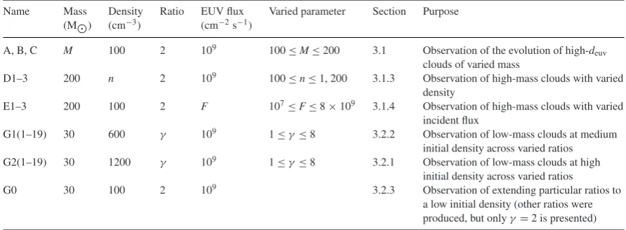
Table 1. Summary of the parameters of all tests examined. After the name of the test series, the next four columns (mass, density, ratio and EUV flux) are the defining parameters of each simulation set. For all series, three of the four are fixed values, and the remaining parameter is represented by a variable, whose range is described in the ‘varied parameter’ column. The final column indicates the main section/subsection in which the test series is discussed.
Name Mass Density Ratio EUV flux Varied parameter Section Purpose (M) (cm−3) (cm−2s−1)
A, B, C M 100 2 109 100≤M≤200 3.1 Observation of the evolution of high-d euv clouds of varied mass
D1–3 200 n 2 109 100≤n≤1, 200 3.1.3 Observation of high-mass clouds with varied density
E1–3 200 100 2 F 107≤F≤8×10⁹ 3.1.4 Observation of high-mass clouds with varied incident flux
G1(1–19) 30 600 γ 109 1≤
γ≤8 3.2.2 Observation of low-mass clouds at medium initial density across varied ratios G2(1–19) 30 1200 γ 109 1≤γ≤8 3.2.1 Observation of low-mass clouds at high
initial density across varied ratios
G0 30 100 2 109 3.2.3 Observation of extending particular ratios to
a low initial density (other ratios were produced, but onlyγ=2 is presented)
orders of magnitude. In the ionized gas regions, recombination of the electrons with ions and the collisional excitation of OIIlines are the dominant processes in the cooling rate function; in the cooler, unionized regions, it is dominated by CO, CI, CIIand OIline
emis-sions.
2.2 Initial and boundary conditions
All of the molecular clouds in our simulations start with a uni-form density, which is rendered by a glass-like distribution of SPH particles created usingGADGET-2 (Springel2005). Compared with
a uniform random distribution, a glass-like distribution has a sub-stantially lower noise in the resulting density distribution. This is of particular benefit in circumstances where small variations are likely to be amplified in the resulting evolution. The number of SPH par-ticles for each molecular cloud is decided according to the mass resolution required by the convergence test of the code II, 10−3M
per SPH particle. A zero initial velocity field is set for all of the molecular clouds in the simulations.
We investigate the dynamic evolution of a prolate cloud with its semi-major axis perpendicular to the incident direction of EUV radiation as shown in Fig.2. Rather than specifying the initial geometry of the prolate cloud by semi-major and semi-minor axis (a,b), we use (a,γ = a
b) as the pair of initial geometrical parameters
for the cloud. The objective of this investigation is to observe the EUV radiation triggered collapse of a prolate cloud; therefore, we set the initial geometric parameters of a prolate cloud of massMin such a way that it would be stable without a radiation field. The Jeans criteria (in terms of Jeans numberJ) for an isolated prolate cloud to be stable against its own gravity can be expressed as (Bastien 1983)
J= πGρμb
2
15eRgT
ln
1+e
1−e
≤1, (1)
whereρ,b,Tandμare the mass density, the minor axis, the initial temperature and the mean molecular mass of the prolate cloud, respectively,GandRgthe gravitational constant and specific gas
constant, and with the eccentricitye=
1−b2
a2 = √
γ2−1
γ .
Substituting ρ=(3M)/(4πab2) into equation (1), we get the
[image:3.595.311.547.277.489.2]condition for the major axisaof an isolated non-collapsing prolate
Figure 2. The projected two-dimensional diagram (on toxzplane) of the initial geometry of a prolate cloud and the configuration of the ionizing (EUV) radiation flux from nearby star(s). The isotropic interstellar back-ground FUV is not drawn in the diagram but considered in simulations.
cloud
a≥acrit=
μGM
20RgT e
ln
1+e
1−e
=0.052 M
∗γ
T γ2−1ln
γ+γ2−1
γ−γ2−1
, (2)
whereM∗is the mass of the prolate cloud in units of solar masses, andaandacrithave units of parsecs. For a given molecular cloud
of massM∗, and initial temperatureTandγ, a minimum value ofa
can be estimated; the major axis of an initially gravitationally stable cloud should satisfya>acrit.
All of the prolate clouds investigated were subject to an isotropic interstellar background FUV radiation of one Habing unit (Habing 1968) and an ionizing EUV radiation with a flux of 109cm−2s−1
z-axis (along the negativez-direction) as illustrated in Fig.2, in which the isotropic interstellar background FUV radiation is not shown, although it is included in our simulations. The boundary condition takes the form of a spherical outflow boundary, with a weak boundary pressure.
2.3 Core-finding program
Because of the occurrence of fragmentation in the evolution of the prolate clouds in our simulations, the number and locations of con-densed cores will provide useful information on the potential sites for EUV radiation triggered star formation. The physical properties of cores formed are derived by using a core-finding code developed to recursively ‘grow’ a candidate core outwards from a high-density particle, connecting in a tree-like structure to nearby particles of lower density.
A ‘core’ in this context is defined as a region surrounding a local density maxima with a peak H2number density greater than 106
cm−3. This results in selection of ‘cores’ with a wide range of peak
densities, from just over 106cm−3up to the code’s effective limit
of≈1013cm−3. The occurrence of the upper limit on the number
density is because the Courant–Friedrichs–Lewy condition time step used in the code becomes extremely small when a high density of 1013 cm−3 is approached. No sink-particle implementation is
implemented in the code, which makes the simulation almost cease to evolve much further after the formation of the first few high-density cores. We use this as the definition of the ‘end’ of the simulation, wherever subsequently referred to. Therefore, our main interest is to explore the effects of the initial conditions of a prolate cloud on its dynamical evolution up to the first batch of proto-star seed formation. In the following, we present the main frame work of the core-finding code.
To begin with, all particles below a density threshold (n<106
cm−3) are discounted. Following this initial filter of particles, the
cores are determined in the following procedures:
(i) The code generates nearest-neighbour lists for every particle. A set of 45 neighbours, the same asNneighfor the SPH code, will be
located and selected for the use of the code presented here. (ii) The particle with maximum density is selected and acts as the seed for the first core.
(iii) The code then searches outwards to select all of the nearest-neighbour particles which have a density lower than the seed par-ticle. From each of these neighbours, the selection process then attempts to search further outwards for any lower density neigh-bours which have not already been selected. Each particle is added to a list for the current seed as they are selected. Two exceptions exist which permit selection of a particle of a higher density than that of the current particle. The first is an ‘overdensity’ margin which was set as 1 per cent of the current density, to select individual spuriously overdense particles. The second is that any connected particles will be automatically selected, regardless of relative number density, if they are above the jeans density limit described by Bate & Burk-ert (1997). This is the density above which artificial fragmentation is expected to occur, and the selection process ensures that local density maxima separated by greater than this density are jointly selected as a single core.
(iv) The selection process continues until no particles remain which are (a) lower number density than the last seed particle (plus the two exceptions) and (b) not already selected by the current seed. (v) This procedure is then repeated from step (ii). This time the new seed particle is selected as being the next maximum density
particle which has not already been selected by a previous descent along nearest-neighbour branches. This is done until no particles remain which can be selected, having been ruled out by one or more of the previously described criteria. Note that particles already selected and labelled by one seed may also be selected and labelled by another seed. Each particle builds up a list of which seeds have selected it.
(vi) Through this process, particles are selected in groups grow-ing out from all localized density maxima. Followgrow-ing the selection of all possible candidate groups, mean properties for each group are determined (position, density, i.e. collective properties of any attribute possessed by the component particles).
(vii) An additional point of note regards particles which were selected and labelled from multiple seeds. In the current implemen-tation, the properties of any particle which is part of more than one seed descent are equally weighted between those seeds. A more comprehensive process for deciding ‘ownership’ of each particle will be implemented in the near future.
The method presented here may provide an advantage in deter-mining non-spherical or highly asymmetrical cores, for which a radial selection or search may not be sufficient. It additionally per-mits determination of structure shapes which are of highly irregular geometries. These include filament and clump features for simu-lations involving larger scale, clumpier structures than those dealt with in this paper, for the approximate shape, size and extent of each core can be determined in the code.
2.4 The EUV flux penetration parameter
The role of the intensive ionizing radiation flux on the evolution of molecular cloud is manifested in two important ways. As stated in the RDI model, an ionizing radiation-induced shock compresses the neutral and cool gas in a molecular cloud into condensed cores which may collapse to form stars under its enhanced self-gravity. At the same time, ionizing radiation-induced photoevaporation erodes gas material from the surface of the cloud, which weakens the potential for star formation. Whether a pre-existing cloud could be triggered to form stars or totally photoevaporated depends on the two competing effects of an EUV radiation field.
To classify the dynamic region of a prolate cloud with specified initial conditions, we define a dimensionless quantity – the EUV radiation penetration parameter, which is the ratio of the physical ionizing radiation penetration depth to the semi-minor axis of a prolate cloud,
dEUV=
FEUV
αBn2
a γ
=1.6×10³F ∗
EUVγ
n2a∗ (pc), (3)
where the major axis a∗ is in the unit of pc,FEUV∗ is the EUV ionizing radiation flux in units of 109cm−2s−1,
αBis the
recom-bination coefficient of hydrogen ion – electron under the ‘on-the-spot’ approximation (Dyson & Williams1997) and has the value of 2.0×10⁻¹³cm3s−1at a temperature of about 104K (Dyson &
Williams1997). This is then taken as a constant, as the equilibrium temperature for ionized material is≈104K and the dependence of
αBon temperature is not strong in the region around that
tempera-ture.
ionizations, respectively), used by Lefloch & Lazareff (1994,1995) for characterization of an ionization shock propagation scenario.
In a normal HIIregion, if the EUV radiation penetration depth is
about one hundredth of the minor axisa
γ, i.e.dEUV<1, the cloud is
in the shock-dominated region and would collapse towards the geo-metrical focus or foci at the final stage of its evolution and we define this mode of the RDI triggered collapse as ‘foci convergence’. In this case, an initially spherical cloud would collapse towards the central point of its final structure, and an initially prolate cloud would collapse towards the two foci, the gravitational centres of the cloud. As the value ofdEUVincreases, but still much less than 1,
the gravitational foci convergence of the cloud is weakened by pho-toevaporation and the cloud collapses towards its major axis. We define this mode of the RDI triggered collapse as ‘linear conver-gence’. Under the very extreme condition ofdEUV→1, the cloud is
in photoevaporation dominant region, and shall totally disperse into its surroundings during its evolution process. We are only interested in investigating the evolution of the prolate clouds which are not in photoevaporation dominant region. From our simulation results, we find thatdEUVis a useful diagnostic parameter to indicate the
evolution of a prolate cloud under the effect of EUV radiation. As the distance scales of the ionization front are generally smaller than an SPH particle smoothing length, it must be treated such that the ionization front progress through the mass of an SPH particle is tracked, rather than resolved spatially. This is done through the implementation of the grid-based method described in section 3.2.2 of Kessel-Deynet & Burkert (2000). The extinction of radiation to a given SPH particle is performed using ray tracing to produce a series of line segments along which the radiation is attenuated. The target SPH particle is then assumed to be a uniform sphere with the radius being defined by its mass and density. The time evolution of the ionization fraction of each particle is computed from solving the ionization and recombination equilibrium equation. This allows an ionization fraction expressed as the equilibrium position of the frontwithinthe smoothing lengths of the particles.
3 R E S U LT S A N D D I S C U S S I O N
Nelson & Langer (1997) investigated the dynamic evolution of three prolate clouds of masses 100, 150 and 200 M, subjected to an isotropic interstellar background (FUV) radiation of one Habing unit (Habing1968). All three clouds collapse to a high-density spindle at the late stage of the evolution. It is our first interest to investigate what effect an additional plane-parallel ionizing EUV radiation field would cause on the evolution of these prolate clouds. This is followed by a systematic exploration on the roles played by initial physical and geometrical conditions of a prolate cloud when subject to the same radiation environment.
All subsequent density cross-section renders of the simulation data in this paper were produced using the ‘SPLASH’ graphical
visu-alization tool (Price2007).
3.1 Evolution of high-mass prolate clouds
The three clouds under investigation are of same initial density, 100 cm−3, and axial ratio of
γ =2. Their properties are listed in Table2, from which it can be seen that each semi-major axis,a, is greater thanacritindicating that they are supported against purely
gravitational collapse.
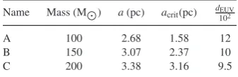
[image:5.595.344.513.123.178.2]We first discuss the evolution of cloud C and then describe the general evolutionary features of clouds A, B and C. The numbers of SPH particles used in the simulations are 100, 150 and 200 thousand
Table 2. The parameters of the three prolate clouds of similar initial uniform density of 100 cm−3 and axial ratioγ=2. The columns, from left to right, are the name, mass, major axis lengtha, the critical ma-jor axis length and the ionizing radiation penetration depth parameter (calculated with equations 2 and 3). Name Mass (M) a(pc) acrit(pc) dEUV
102
A 100 2.68 1.58 12
B 150 3.07 2.37 10
C 200 3.38 3.16 9.5
for clouds A, B and C, respectively, to satisfy the minimum mass resolution requirement, 10−3M
per SPH particle.
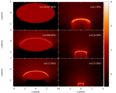
3.1.1 Cloud C – evolutionary features
Fig.3shows six snapshots of the cross-sectional number density evolution in the mid-plane for the molecular cloud C over 0.33 Myr. As time progresses from the start of the simulation, the ioniza-tion heating-induced shock propagates into the cloud through the upper-half ellipsoidal surface (the star-facing side), which is much stronger than that surrounding the lower-half ellipsoidal surface caused by FUV only. The shocked thin layer is very distinctive when
t=0.13 Myr. At the same time, EUV radiation has photoevaporated much of the gas material from the surface of the cloud, such that the overall dimension of the cloud greatly decreases. With the shock propagating into the neural cloud, the condensed thin shell starts to fragment att=0.2 Myr due to its gravitational instability. The densities of the gas between the fragments are lower than that in the fragments and are therefore pushed into the cloud by the high pres-sure in the HII region, to form spike-like microstructures. These
microstructures have higher density than the neutral interior of the cloud, but would not play a significant role over the evolu-tion of the whole system because of their very small volume. At 0.33 Myr, the remaining material has evolved to a clumpy linear structure of≈1 pc in length, along which multiple condensed cores are embedded. The peak density increases from 102cm−3 at the
beginning of the simulation to≈1013cm−3att=0.33 Myr.
In order to obtain a better impression of the distribution of high-density material in the final linear structure, we plot the axial mean density distribution along thex-axis, similar to the method used by Nelson & Papaloizou (1993) and Nelson & Langer (1999). We divide the length of the prolate cloud along the major-axis intoK
bins of equal length 2a/K. We then calculate the mean hydrogen number density for the SPH particles in the bin, i.e. ¯ni=
jnj
Ni
for theith bin along the x-axis, withi = 1, 2, 3, . . . ,K, Ni is
the number of SPH particles of theith bin andjis the index of all particles within each bin. ¯niprovides a clear view of the distribution
of high-density material. Results for the shape of the distribution are converged for a wide range of bin widths relative to smoothing lengths (20 < K < 2400 provides identical overall shapes with varying detail for cloud C).K=150 was used for the distributions presented here.
Figure 3. Sequence of the evolution of the mid-plane cross-sectional number density for cloud C, of initial density 100 cm−3andγ =2.0, subject to an isotropic interstellar background radiation and ionizing radiation with the configuration shown in Fig.2. Time sequence is top to bottom and then left to right.
grid plus arithmetic average over the grids in anx-bin is found to be insufficient, because it does not highlight the high-density regions at all.
We would like to emphasize, however, that it is a qualitative illustration of general high-density material distribution, rather than a quantitative representation of core locations and properties, for which the analysis with the core-finding program is used.
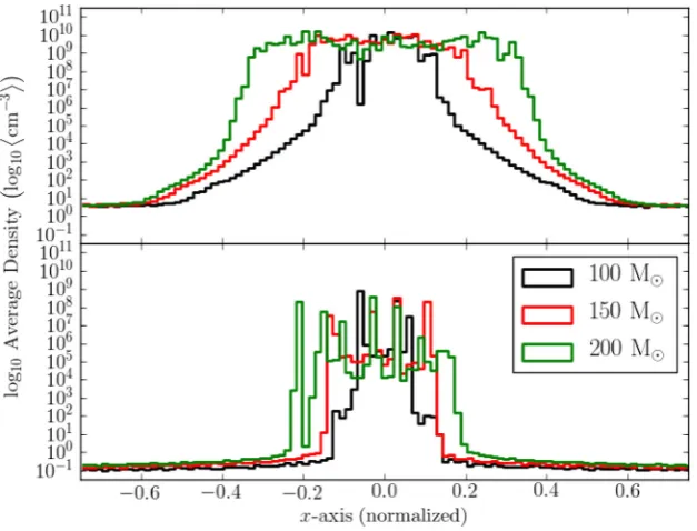
For a comparison, we also plot the evolved final axial mean density distribution for the same cloud but without EUV radiation (Nelson & Langer1997). The green lines in the two panels of Fig.4 describe the distribution of ¯ni along the major axis (x) of cloud
C without (upper panel att= 3.03 Myr) and with (lower panel at 0.33 Myr) EUV radiation. An obvious difference which can be seen from these two profiles is that the EUV radiation-induced shock could trigger distinctive density peaks along the final linear structure, while most of the less dense material between the cores is blown away by the strong EUV-induced photoevaporation. It is worth noting that an apparent high-density peak in these plots does not necessarily correspond to a single high-density core; multiple cores may be present at differentyandzpositions within the same
x-axis bin. In comparison, the FUV-only radiation-induced shock is much weaker than that of EUV radiation. As such it is about 20 times slower at compressing the gas. Also there are no well-separated high-density peaks appearing in the FUV-only radiation case. We believe that this may be because the FUV radiation is isotropic and the induced weak shock effect is symmetrical about the major axis.
3.1.2 Clouds A, B and C – common and different evolutionary features
For the other two clouds A and B, similar morphological evolution to that of cloud C is observed. Plotted in Fig.4are their axial mean density distributions along the major axis at the final time step of each simulation.
It is apparent that the high-density cores in all three simulated clouds including EUV radiation scatter over the final clumpy lin-ear structure unlike their corresponding non-EUV simulations. In the FUV-only cases, the high-density material is more evenly dis-tributed along the final spindle structure. Also apparent in Fig.4is that more gas material remains in the linear structure in the simu-lation without EUV radiation than that with EUV radiation. This is because the EUV radiation flux is more than 20 times more ener-getic than the interstellar background FUV radiation, the consequent photoevaporation effect is stronger in a similar proportion. Further-more, the number of distinctive peaks increases with the initial mass of the cloud. This is understandable as the major axis is longer in higher mass clouds to keep the same initial density, accompanied with an increase in mean mass per unit length. Fragmentation of a longer structure produces more individual fragments.
These highly condensed peaks can be considered to be poten-tial sites for further star formation. The scattered distinctive high-density cores over the remaining linear structure imply that EUV radiation may be able to trigger a chain of stars to form in the ex-amined prolate clouds at an HIIboundary in less than 0.5 Myr. In
Figure 4. Mean hydrogen number density along the semi-major axis of three prolate clouds of initial density 100 cm−3and varying masses. Frame (a) is for the three clouds subject to an isotropic FUV radiation only; frame (b) is for the same three clouds subject to both FUV and EUV radiation fields. The time-scales for the clouds in frame (a) are 3.10, 3.02 and 3.03 Myr for the clouds of 100, 150 and 200 M, respectively, and 0.33 Myr for all of the clouds in frame (b).
Table 3. The parameters of the further exploration high-mass prolate clouds. The columns, from left to right, are the name, density, major axis lengtha, incident EUV flux and the ion-izing radiation penetration depth parameter (calculated with equations 2 and 3). Time indicates the final simulation time. Cloud C is the same as in the previous section; clouds D1–3 are the additional density-varied tests, and clouds E1–3 are the additional incident flux-varied tests.
Name Density a Flux dEUV Time
(cm−3) (pc) (cm−2s−1) (10−2) (Myr)
C 100 3.38 109 9.5 0.334
D1 400 2.13 109 0.93 0.327
D2 600 1.86 109 0.48 0.288
D3 1200 1.48 109 0.15 0.233
E1 100 3.38 107 0.095 0.966
E2 100 3.38 108 0.95 0.776
E3 100 3.38 8×10⁹ 76 0.268
are more likely to form a condensed filamentary structure under the effect of the FUV-only radiation over a period of a few Myr.
3.1.3 D series – effects of varied initial density
In order to inspect how the evolutionary destiny would change if the initial density of the above prolate cloud is increased, we investigated the evolution of another three prolate clouds which have the same mass of 200 M, but different initial densities. These tests are labelled D1–3 in Table3.
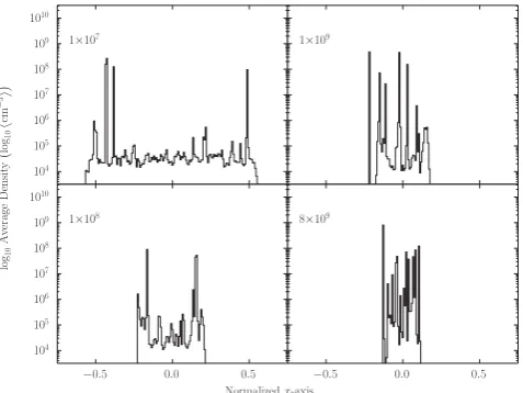
Presented in Fig.5are the axial mean density distributions along the formed linear structures at the final time step. The plot for cloud C is also shown for comparison. It is interesting to see that with increasing initial density, the condensed cores gradually move to-wards the two foci or say the two ends of the final filament structure. This is because the ionizing radiation penetration depth parameter
Figure 5. The axial mean number density profile at the final time steps in four molecular clouds of same mass of 200 M, andγ=2, but different initial densities as shown in the top-left corner in each panel. The densities are in units of cm−3. The times at which the simulations ended are shown in Table3.
decreases with the increase of the initial density; the mode of the evolution of the cloud changes from linear to foci convergence.
3.1.4 E series – effects of varied EUV flux
[image:7.595.69.264.442.546.2]Figure 6. The axial mean number density profile at the final time steps in four molecular clouds of same mass of 200 M,γ=2 and initial density of 100 cm−3, but under the effect of different EUV radiation fluxes as shown in the top-left corner in each panel. The fluxes are in units of cm−2s−1. The times at which the simulations ended are shown in Table3.
increase ofdEUV. The mode of the evolution of the cloud changes
from foci to linear convergence.
Next, we turn to a systematic investigation on the evolutionary features of prolate clouds of an intermediate initial mass of 30 M, a typical initial density around 103cm−3and different initial shapes.
3.2 Evolution of prolate clouds of 30 M
The prolate clouds in this investigation have masses of 30 M, different initial densities of 600 and 1200 cm−3, and varied initial
geometrical shapes defined by the axial ratio parameter 1 ≤ γ ≤ 8. We categorize them into two groups G1 and G2, as listed in Table 4. Their initial major axes are all larger than theiracrit,
which means they are all stable against purely gravitational collapse. There are 19 clouds in each group and are numbered from 1 to 19. The identification for each cloud is notated as G1(No.) and G2(No.), e.g. the fifth cloud in the G2 series is named G2(5). Each of the simulations for the 38 clouds was run with 105SPH particles,
leading to a mass resolution of 3.0×10⁻⁴M
per SPH particle, a higher resolution than required by the convergence tests (10−3M
per SPH particle).
In the following, we present the simulation data and analyse the features of the evolutionary sequence for the two groups of prolate clouds.
3.2.1 G2 series – effects of varied initial geometry
The morphological evolution of the clouds in the G2 group are very similar to each other, so we only describe in detail the evolutionary sequence for the cloud G2(5), which is of an initial axial ratio of 2 and an initial density 1200 cm−3. Then, we have a general
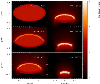
description of the evolutionary features of the whole group. The six panels in Fig. 7describe the evolution of the cross-sectional number density in the mid-plane (x−zandy= 0) of the cloud G2(5). The morphological evolution appears to follow the general picture described by the RDI mechanism. A condensed gas layer at the upper ellipsoidal surface has formed within 0.11 Myr. The density inside the shocked layer increases as it propagates
Table 4. Parameters of two groups of molecular clouds of same mass but different initial densities of 600 and 1200 cm−3. From left to right, columns 1–3 are the number identity, axial ratio and the critical semi major axis defined by equation (2) for both G1 and G2 clouds. Columns 4 and 5 are the major axis anddEUVdefined by equation (3) for the G1 clouds, and columns 5 and 6 are the same parameters for the G2 clouds. All of the semi-major axes and critical semi-major axes are in units of pc and the penetration depth is unitless.
G1 G2
No. γ acrit a600 d10EUV2 a1200 d10EUV2
1 1.000 0.052 0.623 0.713 0.494 0.225
2 1.250 0.060 0.722 0.770 0.573 0.242
3 1.500 0.067 0.816 0.817 0.648 0.257
4 1.750 0.073 0.904 0.860 0.718 0.271
5 2.000 0.079 0.988 0.900 0.784 0.283
6 2.250 0.084 1.069 0.935 0.849 0.294
7 2.500 0.039 1.147 0.969 0.910 0.305
8 2.750 0.093 1.222 1.001 0.970 0.315
9 3.000 0.097 1.295 1.030 1.028 0.324
10 3.250 0.101 1.366 1.057 1.084 0.333
11 3.500 0.104 1.435 1.084 1.139 0.341
12 3.750 0.107 1.503 1.109 1.193 0.349
13 4.00 0.110 1.569 1.133 1.245 0.357
14 4.50 0.116 1.697 1.179 1.347 0.371
15 5.00 0.121 1.820 1.221 1.445 0.384
16 5.50 0.126 1.940 1.260 1.540 0.397
17 6.00 0.130 2.056 1.297 1.632 0.408
18 7.00 0.138 2.278 1.366 1.808 0.430
19 8.00 0.145 2.490 1.428 1.977 0.450
inwards. Att≈0.19 Myr, the highly condensed layer fragments, cre-ating a curved clumpy filamentary structure with condensed cores embedded. The corresponding overhead (x−y) view of the evolu-tion of the cloud displayed in Fig.8further confirms the formation of the filamentary structure and its fragmentation. It is seen that the filamentary structure forms as a high-density ‘spine’ aligned with the semi-major axis att=0.11 Myr. The material in the two hemi-spheres is seen converging to the majorx-axis, and material from negativeyheads towards the positivey-direction, and vice versa. Att=0.15 Myr, this thin and long structure starts fragmentation. Some of the fragments disperse off the major axis, and a broadly zigzag fragment-core structure is left att=0.19 Myr.
The red line in Fig.9describes the axial mean density distribution att=0.19 Myr. It shows distinctive high-density peaks forming at the two ends of the filamentary structure. The penetration depth parameter of cloud G2(5) isdEUV =0.283 per cent as shown in
Table4, which means that EUV radiation-induced shock dominates the evolution of G2(5) and enhances the self-gravity of the cloud G2(5) so that most of remaining condensed gas is driven towards the two foci of the cloud over its evolution (foci convergence).
[image:8.595.306.547.143.369.2]Figure 7. Evolution of the cross-sectional density in the mid-plane for the prolate cloud G2(5) over 0.19 Myr. Time is displayed in the upper right of each panel. The order of time evolution is top to bottom and then left to right.
[image:9.595.92.500.422.656.2]Figure 9. The axial mean number density profile for clouds G1(5) (600 cm−3,γ=2) in solid black and G2(5) (1200 cm−3,γ=2) in dashed red. G1(5) is att=0.22 Myr and G2(5) att=0.19 Myr.
when the gravitational centre changes from one to two. However, in the clouds of initial 3 < γ ≤ 10.0, the core collapsing time decreases from 0.21 to 0.15 Myr withγ. This may be because the initial cloud havingγ >3 becomes more and more elongated; with
γ increasing, the converging gas material has shorter and shorter distance (therefore shorter converging time) to travel to collapse towards their two foci. Therefore, spherical and highly ellipsoidal clouds have shorter core formation than those of the mid-range of axial ratios (this can also be seen in Fig.15).
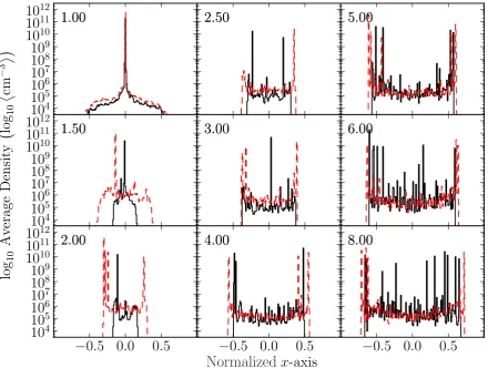
It is also of interest to look at the axial mean density profiles of a set of clouds in the G2 group. The red dashed lines in Fig. 11 reveal the location of the high-density peak(s) triggered by the EUV radiation flux for nine clouds selected from the G2 group (the
axial ratio for each is displayed in the upper left of the panel). An initially spherical cloud G2(1) converges to its gravitational centre to form a single dense peak as shown in the first panel. As axial ratio increases, high-density cores are forming at the two ends of the final structures. The G2 group clouds all havedEUV<0.5 per
cent and therefore all collapse in the mode of foci convergence.
3.2.2 G1 series – effects of varied initial geometry with halved initial density
The clouds in the G1 series have an initial density of half that of the G2 group, 600 cm−3. Their EUV radiation flux penetration
parameters are in the range 0.713≤dEUV<1.428 per cent, larger
than that of all of the clouds in G2 group.
The morphological evolution of G1 group clouds is similar to that of G2 group clouds. Clouds ofγequal or close to 1 form type B or type A BRCs with a single core forming at the its head. Asγ
increases, the clouds evolve into filamentary structures with cores embedded inside. For even higher axial ratios, warm but dense capillary structure appears ahead of the shocked layer as seen in cloud C as well. The axial mean density profiles for nine G1 group clouds are plotted as black solid lines in Fig.11, which describe a coverage of all dynamic features of the G1 series.
As seen from Fig.11, the clouds of 1≤γ <2.0 and 0.713≤
dEUV<0.9 per cent in both groups are spherical or quasi-spherical
and evolve to similar structures with a highly condensed core, except more gas material is evaporated from G1 group clouds compared to the G2 group clouds. This is shown by the narrower density profile when compared with the G2(1–4) clouds. The above feature can be explained by the higher values ofdEUV in G1 clouds, where
more surface material is photoevaporated. However, the overall dynamical evolution of these clouds can still be categorized as shock dominant, as most of remaining material in the cloud converges to the gravitational centre of the BRCs.
[image:10.595.92.499.445.704.2]Figure 11. The axial mean density over thex-axis (normalized to the initial cloud semi-major axis) for nine of the G1 (black solid line) and G2 (red dashed line) series clouds. The number in the upper left of each panel is theγvalue of the clouds.
Clouds of 2≤γ <6.0 and 0.90 ≤dEUV < 1.26 per cent in
the G1 group not only develop highly condensed cores at one or both ends of the final filamentary structure, but also between the two foci, especially the middle core in the cloud G1(9) ofγ =3 has a much higher mean density than the sides cores in the same cloud. The above feature suggests that the EUV radiation-induced shock dominance decreases. As such, the gravitational convergence towards the two foci is gradually weakened and more gas collapses towards the major axis to form a filament, which then fragments into a few dense cores. It appears that their collapse modes are in a transition region between foci convergence and linear convergence. The clouds having axial ratios 6.0≤γ ≤8.00 anddEUV>1.26
per cent all collapse in the mode of linear convergence, and the condensed cores spread over the final filamentary structure. For example, in the cloud ofγ =8.00 anddEUV=1.43 per cent,
con-vergence towards two foci has broken; the high-density cores have similar a mean peak density to the consequence of the fragmentation of the final filamentary structure.
3.2.3 Effects of varied cloud ratio and lower densities
To confirm the correlation observed betweendEUVand the
evolu-tionary destiny of a cloud, two additional sets of simulations were run with prolate clouds of 30 M, but of lower initial densities, 300 and 100 cm−3. Each group has four different clouds of
γ=1.5, 2.0,
2.5 and 4. With these initial conditions, the 300 cm−3clouds have
an ionizing depth parameter of 2.6≤dEUV≤3.6 per cent, and for
the clouds of 100 cm−3, 16≤d
EUV≤22 per cent. In total, eight
simulations were run with the same mass resolution as used in the G1 and G2 series simulations.
The morphological evolution and the axial mean density profiles are qualitatively similar to that of the highly ellipsoidal clouds in the G1 simulations, so we do not present similar plots to Figs10 and11. None of them collapse in the mode of foci convergence. We select a representative from the eight simulations to compare its mode of convergence with that of the G2(5) and G1(5) clouds illustrated in Sections 3.2.1 and 3.2.2, respectively. The cloud with initial density of 100 cm−3,
γ=2 anddEUV=17.8 is chosen, and
will be notated as cloud G0.
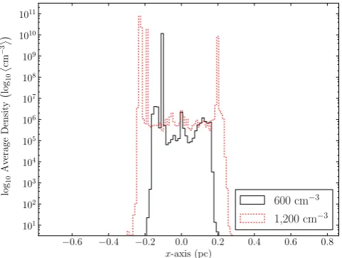
Fig.12 shows a comparison of the axial mean density profile over the normalizedx-axis for three molecular clouds of γ = 2,
M=30 M and different initial densities of 100 (black line for G0), 600 (red for G1(5)) and 1200 (green for G2(5)) cm−3. It is
clearly seen again that the mode of collapse in the three clouds changes from linear convergence in G0, to foci–linear mixture con-vergence in cloud G1(5), then to foci concon-vergence in G2(5), with
dEUVdecreasing from 17.8 to 0.28 per cent.
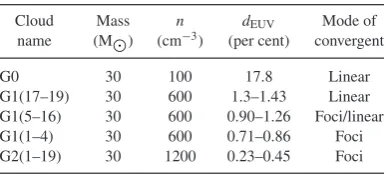
Table5presents a summary on the evolutionary destiny of all the investigated clouds in this series, related to the diagnostic parameter
Figure 12. The axial mean number density distribution for molecular clouds of 30 Mandγ=2 but different initial densities. The legend boxes describe the line style and colour correspondence for the densities of the featured clouds, G0 (100 cm−3), G1(5) (600 cm−3) and G2(5) (1200 cm−3). The evolutionary times of the clouds featured are 0.25, 0.22 and 0.19 Myr for G0, G1(5) and G2(5), respectively.
Table 5. A summary of the evolutionary destiny of the molecular clouds of mass 30 M.
Cloud Mass n dEUV Mode of
name (M) (cm−3) (per cent) convergent
G0 30 100 17.8 Linear
G1(17–19) 30 600 1.3–1.43 Linear
G1(5–16) 30 600 0.90–1.26 Foci/linear
G1(1–4) 30 600 0.71–0.86 Foci
G2(1–19) 30 1200 0.23–0.45 Foci
3.2.4 The location of cores
From the above investigation, it is known that high-density cores formed in clouds of lower dEUV (≤1.25 per cent) tend to locate
around the two ends (foci) of the final filamentary structure. Now investigated are the detailed location profiles of condensed cores along thex-axis using the core-finding program described in Sec-tion 2.3. For this objective, we are only interested in the cores with a peak density (nc) higher than 108cm−3, which can be taken as
the potential seeds for new stars to form (Nelson & Langer1997). In each panel, the short horizontal lines specify the initial extent of the semi-major axis along thex-direction for clouds of theγ and initial density specified in the plot.
Plotted in Fig.13are the distributions of condensed cores in G1 and G2 clouds of differentγ. The derived data of cores from the core-finding process have been further filtered by the peak den-sity,nc(≥108cm−3in all cases described here), and a minimum
mass thresholdmc. The two panels on the left have a selection of
mc≥0.06 M, and the two on the right ofmc≥0.2 M. The
x-displacement parameter is the modulus of thex-axis position of the peak of the core, |xc|. Within each panel, two peak density
regimes are distinguished by white filled circles, indicating a den-sity of 108≤
nc≤1012cm−3, and black filled circles fornc>1012
cm−3, being cores of extremely high density. It is seen from each
panel in Fig.13that extremely high density cores only form in the clouds of lowerγvalues and appear at the focus points.
In the two panels on the left, wheremc≥0.06 M, the upper of
these is for the G2 series of clouds, and the lower for the G1 series. With increasingγ, high-density cores form mainly around the foci of the ellipsoidal cloud in G2, but appear scattered over the whole cloud length in some of the G1 clouds.
The results for the higher core mass criteria (mc>0.2 M) are
presented in the two panels on the right of Fig.13. The upper of these being the G2 series of clouds, and the lower the G1 series. It is seen that the high-mass cores in all clouds of the G2 series are located at the centre or foci along thex-axis. The picture is not so simple in G1 clouds. In clouds ofγ ≤2, high-mass cores appear close to the centre pointx=0. Some clouds ofγ >2 have the high-mass cores at two foci and closer to the middle of thex-axis as well. Some more ellipsoidal clouds have high-mass core(s) either at/around the foci or spread between the foci. A few of the higher
γclouds in G1 have no core(s) with mass higher than 0.2 M. The general picture that is revealed is that the clouds in the G2 and the low-γclouds in the G1 groups have almost all of their cores located around their foci. Clouds of higherγ values in G1 have their condensed cores spread along thex-axis. The different core distributions between these clouds can be explained by the lower
dEUVin the G2 and low-γ G1 clouds compared to the high-γ G1
clouds.
3.2.5 The total core mass and core formation time
In order to evaluate the efficiency of EUV radiation triggered poten-tial star formation in the different prolate clouds of the G1 and G2 groups, we compare the total mass of dense cores and the time for high-density core formation in clouds of differentγin both groups. Plotted in Fig. 14 is the variation of the total mass of high-density cores in a cloud,mtot, withγ for both groups. It is clearly
seen that for each pair of G1 and G2 clouds of the sameγ,mtotfor
the G2 cloud is more than double that of the G1 cloud. G1 group clouds have higherdEUVand therefore lose more material through
photoevaporation. The range ofmtotis 1–4.85 Min the G2 series
and 0.05–2.2 Min the G1 series.
However, the variation ofmtotoverγ in each individual group
is non-monotonic. Taking G2 group as an example, the spherical cloud has highest degree of convergence, so it has the maximum total core mass. When 1< γ ≤1.5, although the cloud becomes an ellipsoid, the two foci are still very close to each other that their effect on gathering gas towards them is similar to one focus cloud. This can be confirmed by the single high-density peak in the corresponding axial mean density distribution (in red lines) in Fig.11. The final structure still keep the morphology of a single BRC as shown in Fig. 7. When γ increases to 1.5, the overall gravitational convergence towards the centre of mass decreases, so the total core massmtotof the high-density core decreases withγ,
to the value of 2.6 M.
When 1.75≤γ ≤2.25, the distance between the two foci in a cloud increases to such a degree that two foci convergence becomes obvious, as shown in the corresponding panels (in red lines) in Fig.11; the morphology of the final cloud is no longer a single BRC but a linear structure as shown in Fig.7. Now there are two gravitational converging centres to accrete gas, so the total core mass shows a sharp increase to 4.2 Min cloud havingγ =1.75, then slightly increases withγ up to 4.85 Min the cloud having
γ=2.25.
Figure 13. x-displacement locations (|xc|) of condensed cores formed in the G1 and G2 cloud series with different criteria on the threshold of core massmc.
nis the initial density of the clouds whose cores are sampled in the corresponding panel. The short horizontal line for eachγexamined denotes the initial semi-major axis of the cloud. The white circles indicate cores of density 108≤n
c≤1012cm−3and the black circles core densities ofnc≥1012cm−3.
Figure 14. The total massmtotof all cores with selection criteria ofnc≥106 cm−3andm
c=0.06 Mat the end of the simulated evolution for all G1 and G2 clouds.
becomes lower and lower and the gas available to be accreted by the two foci gets less and less. Therefore,mtotdecreases withγjust
as shown in Fig.14.
Fig.15shows the variation of the characteristic high-density core formation time (when the highest density reaches≈1013cm−3, as
[image:13.595.61.277.441.610.2]described in Section 2.3),tcore, overγ for the two group clouds.
Figure 15. The earliest core formation time for all clouds in the G1 and G2 series.
[image:13.595.310.549.441.625.2]Figure 16. Fragment-core structures taken from various sources. On the left is the segment of theHerschelimage of M16 at 60µm. In the upper-right panel is a section of aSpitzerpseudo-colour image of part of IC1848E (Chauhan et al.2011). The lower-right panel shows a segment of a fragment-core structure in a Hubble image of Carina nebula in neutral hydrogen, taken from Hubble website.
densities (of the order of 1012cm−3), meaning that the increase in
starting density alone for the G2 clouds relative to the G1 clouds is unlikely to account for the reduction in formation time.
In both series, spherical clouds can be RDI shocked to form con-densed cores in the shortest time of≈0.125 Myr. Asγ increases from 1, the core formation time increases. This is determined to be because, as the single focus splits towards two foci, collection of material, and subsequent gravitational collapse, becomes slower. We take clouds in the G2 set as an example to look at the variation of
tcoreoverγ. It is seen thattcoreincreases from 0.125 to 0.22 Myr in
clouds of 1< γ≤3. For clouds with axial ratio 3< γ, they become increasingly elongated and the shocked gas has a decreasing dis-tance to travel to collapse towards the foci, and then the time needed for high-density core formation decreases withγ. The variation of
tcoreversusγin G1 clouds is observed to follow a similar pattern to
that in G2 clouds.
3.3 The correlation with observation
Many of the fragment-core structures found at HIIboundaries have
their linear axes perpendicular to the direction of the host star(s). A few examples of such structures are presented in Fig.16. The mor-phology of these structures is very similar to that in the simulations we present in this paper. Object A in the left-hand panel of Fig.16 (a 60μmHerschelimage of M16) is a typical linear structure with two condensed ends, whose morphological image is similar to the simulated structures from G2 clouds. Objects B and C in the same panel, as well as the other linear structures in the upper- and lower-right panels in Fig. 16, have similar morphological structures to clouds A, B, C and several clouds in the G1 series. Therefore, it is reasonable to suggest that these fragment-core structures are the outcomes of the interplay between the EUV radiation from nearby stars and its initial prolate molecular cloud.
However, a quantitative comparison on the physical properties between simulation results and observations is not yet possible at this stage, due to lack of the detailed observational data.
3.4 Link to other modelling work
The fragment-core structures found along HIIboundaries and the
perfect HIIbubble structure (Whitworth et al.1994; Deharveng et al. 2009,2012) were taken as the result of the ‘collect and collapse’ (C & C) mechanism (Elmegreen & Lada1977; Dale, Bonnell & Whitworth2007) in the previous theoretical modelling work. By setting a star in the centre of a uniform spherical cloud, C & C simulation can result in a perfect ‘bubble’-like HIIregion with a
fragment-core inner boundary.
Recently, Walch et al. (2012) performed SPH simulations based on the RDI model, by replacing the uniform-density spherical cloud used in the C & C model with a fractal molecular cloud. Their simulations revealed the formation of a similar HIIbubble structure
with a widespread network of fragment-core structure.
Our simulations show that the fragment-core structure sporadi-cally located along an HIIboundary could also be the consequence
of RDI on a pre-existing uniform prolate cloud with its semi-major axis perpendicular to the ionizing radiation flux.
The RDI and C & C mechanisms are equivalent in terms of the physical interaction process between ionization radiation and a molecular cloud, but they are different in terms of the initial conditions of the molecular cloud used and the relative position of the star to the molecular cloud. A uniform spherical cloud with ionizing star in its centre is used in the C & C model, a fractal and spherical molecular cloud with stars at its centre is used in Walch’s RDI model, and a pre-existing prolate cloud with ionizing stars at its one side is used in our RDI model. The details resolved from different models could explain the variety in the structures of HII
regions observed.
4 C O N C L U S I O N S
Simulation results on three high-mass prolate clouds reveal that a plane-parallel EUV radiation can trigger the formation of distinctive fragment-core structure, in comparison with the formation of a high-density spindle when no EUV radiation is present.
Further investigation on both the high- and low-mass clouds finds that the embedded cores can either spread over the final linear struc-ture or accumulate around the two foci of the cloud, dependent on the initial conditions and radiation fluxes. A dimensionless parame-ter of the EUV radiation flux penetration depthdEUVcan be used as
an indicator to the evolutionary destiny of the clouds investigated. In clouds ofdEUV≤0.86 per cent, the collapse of a cloud is through
foci convergence. The high-density cores mainly locate around the two ends (two gravitational foci) of the linear structure with poten-tial to form two well-separated stars or two groups of stars. In clouds of 0.86<dEUV≤1.26 per cent, the mode of the cloud collapse is a
mixture of foci and linear convergence. The high-density cores are found at one or two ends of the linear structure, while some cores with slightly lower centre density are also found between the two foci. In clouds ofdEUV>1.26 per cent, the cloud collapses in the
mode of linear convergence, when the high-density cores spread over the whole linear structure with potential to form a chain of stars.
Data analysis on the total core mass and core formation time in the two groups of low-mass clouds (the G1 group with initial density of 600 cm−3, G2 with that of 1200 cm−3) find that (i) the
total core massmtotin each of the G2 clouds is more than double
that in each corresponding G1 cloud. (ii) In clouds of same initial density,mtotdecreases whileγ is small (there is only one or
two well-separated foci, and finally decreases again afterγ >2.25. (iii) The characteristic core formation timetcoreis shorter in 95 per
cent of the G2 clouds than that in the corresponding cloud in the G1 series. It increases withγwhenγ ≤3, and then becomes a quasi-constant atγ >3 in both cloud groups. (iv) The spherical cloud has the highestmtotand shortesttcorein both groups of clouds, which
implies that EUV radiation triggered star formation in spherical cloud is most efficient.
As the high-density cores are the potential sites for future star formation, we can conclude that, for prolate clouds with their major axis perpendicular to the same incident EUV radiation: (i) in clouds of the same axial ratio, EUV radiation triggered star formation would be more efficient in the cloud with higher initial density; (ii) in a group of clouds with same initial density, EUV radiation triggered star formation is more effective in clouds of intermediate axial ratio 1.75≤γ <3.
The sporadic core-fragment structures found in multiple HII
boundaries may be taken as the result of RDI in pre-existing prolate clouds, such as investigated here.
In our next paper, we will discuss the evolution of a prolate cloud inclined to the direction of the incident ionizing radiation to address the mechanism for the formation of the BRCs with asymmetrical morphologies.
AC K N OW L E D G E M E N T S
TMK acknowledges a University of Kent scholarship. The authors would like to thank the referees for their beneficial comments in the development of the paper.
R E F E R E N C E S
Bastien P., 1983, A&A, 119, 109
Bate M. R., Burkert A., 1997, MNRAS, 288, 1060 Bertoldi F., 1989, ApJ, 346, 735
Bisbas T. G., W¨unsch R., Whitworth A. P., Hubber D. A., Walch S., 2011, ApJ, 736, 142
Boss A. P., 2009, ApJ, 697, 1940 Cai M. J., Taam R. E., 2010, ApJ, 709, L79
Chauhan N., Pandey A. K., Ogura K., Jose J., Ojha D. K., Samal M. R., Mito H., 2011, MNRAS, 415, 1202
Chauhan N., Ogura K., Pandey A. K., Samal M. R., Bhatt B. C., 2011, PASJ, 63, 795
Choudhury R., Mookerjea B., Bhatt H. C., 2010, ApJ, 717, 1067 Cohen M., Staveley-Smith L., Green A., 2003, MNRAS, 340, 275 Curry C. L., Stahler S. W., 2001, ApJ, 555, 160
Dale J. E., Bonnell I. A., Whitworth A. P., 2007, MNRAS, 375, 1291 Deharveng L., Zavagno A., Schuller F., Caplan J., Pomar`es M., De Breuck
C., 2009, A&A, 496, 177
Deharveng L. et al., 2012, A&A, 546, A74
Dyson J. E., Williams D. A., 1997, The Physics of the Interstellar Medium. IoP Publishing, Bristol
Elmegreen B. G., Lada C. J., 1977, ApJ, 214, 725 Esquivel A., Raga A. C., 2007, MNRAS, 377, 383
Fukuda N., Miao J., Sugitani K., Kawahara K., Watanabe M., Nakano M., Pickles A. J., 2013, ApJ, 773, 132
Gritschneder M., Naab T., Walch S., Burkert A., Heitsch F., 2009, ApJ, 694, L26
Habing H. J., 1968, Bull. Astron. Inst. Neth., 19, 421 Haworth T. J., Harries T. J., 2012, MNRAS, 420, 562 Jones C. E., Basu S., Dubinski J., 2001, ApJ, 551, 387 Karr J. L., Noriega-Crespo A., Martin P. G., 2005, AJ, 129, 954 Kessel-Deynet O., Burkert A., 2000, MNRAS, 315, 713 Kessel-Deynet O., Burkert A., 2003, MNRAS, 338, 545 Lefloch B., Lazareff B., 1994, A&A, 289, 559 Lefloch B., Lazareff B., 1995, A&A, 301, 522 McKee C. F., Hollenbach D. J., 1980, ARA&A, 18, 219
Miao J., White G. J., Nelson R., Thompson M., Morgan L., 2006, MNRAS, 369, 143
Miao J., White G. J., Thompson M. A., Nelson R. P., 2009, ApJ, 692, 382 Miao J., Sugitani K., White G. J., Nelson R. P., 2010, ApJ, 717, 658 Morgan L. K., Thompson M. A., Urquhart J. S., White G. J., Miao J., 2004,
A&A, 426, 535
Myers P. C., Fuller G. A., Goodman A. A., Benson P. J., 1991, ApJ, 376, 561
Nelson R. P., Langer W. D., 1997, ApJ, 482, 796 Nelson R. P., Langer W. D., 1999, ApJ, 524, 923 Nelson R. P., Papaloizou J. C. B., 1993, MNRAS, 265, 905 Nelson R. P., Papaloizou J. C. B., 1994, MNRAS, 270, 1 Ogura K., Sugitani K., 1998, Publ. Astron. Soc. Aust., 15, 91 Ojha D. K. et al., 2011, ApJ, 738, 156
Price D. J., 2007, Publ. Astron. Soc. Aust., 24, 159
Rathborne J. M., Johnson A. M., Jackson J. M., Shah R. Y., Simon R., 2009, ApJS, 182, 131
Sandford M. T., II, Whitaker R. W., Klein R. I., 1982, ApJ, 260, 183 Springel V., 2005, MNRAS, 364, 1105
Sugitani K., Ogura K., 1994, ApJS, 92, 163 Sugitani K., Fukui Y., Ogura K., 1991, ApJS, 77, 59 Sugitani K., Tamura M., Ogura K., 1995, ApJ, 455, L39 Tassis K., 2007, MNRAS, 379, L50
Urquhart J. S., Thompson M. A., Morgan L. K., White G. J., 2006, A&A, 450, 625
Walch S. K., Whitworth A. P., Bisbas T., W¨unsch R., Hubber D., 2012, MNRAS, 427, 625
Whitworth A. P., Bhattal A. S., Chapman S. J., Disney M. J., Turner J. A., 1994, MNRAS, 268, 291