Development of a two dimensional stochastic methodology and a computer model to assess response to the nonlinear seismic wave propagation

Rochester Institute of Technology

RIT Scholar Works

Theses

4-18-2019

Development of a two dimensional stochastic

methodology and a computer model to assess

response to the nonlinear seismic wave propagation

Sudhanshu Sengaonkar

1

ROCHESTER INSTITUTE OF TECHNOLOGY

Development of a two dimensional stochastic methodology and

a computer model to assess response to the nonlinear seismic

wave propagation

Submitted by,

Sudhanshu Sengaonkar

A Thesis Submitted in Partial Fulfillment of the Requirement for Master of

Science in Mechanical Engineering

Department of Mechanical Engineering

Kate Gleason College of Engineering

Approved by:

Dr. Alexander Liberson

---Department of Mechanical Engineering

(Advisor)

Dr. Sarilyn Ivancic

---Department of Mechanical Engineering

(Committee Member)

Dr. Jason Kolodziej

---Department of Mechanical Engineering

(Committee Member)

Dr. Agamemnon Crassidis

---Department of Mechanical Engineering

(Department Representative)

Rochester Institute of Technology

Rochester, New York

2

ABSTRACT

Seismic wave propagation in spatially variable soil continuum can be described by partial

differential equations (PDE) with stochastic coefficients. Typical method of analysis in this area

is a spectral analysis approach, where time series is presented by a Fourier expansion or a

Fourier integral transform. This approach has a limited capability being applicable to the linear

problems only.

The novelty of presented method is that it can handle any nonlinear elastic - plastic stochastic

constitutive model. The output of the project is the 2D seismic random wave propagation model

accounting for the spatial variability of soil properties, described by the linear and nonlinear

constitutive models. This model allows accessing the seismic hazard of a region of interest with

account of its specific geological and topographic features. Time dependent ground velocities,

accelerations, stress components and pressure applied to the walls of an engineering structure

(power plant) have been predicted to estimate the seismic lifeline hazard of engineering facilities.

Nonlinear seismic wave propagations are simulated based on a dynamic two dimensional theory

of mechanics of continuum with account of nonlinear Hencky-Nadai constitutive models.

Boundary conditions relate to the acceleration profile given by accelerometer or seismometer,

zero stress components at the ground surface, free surface conditions at the top and non-reflected

(absorbed) boundary conditions at distal boundaries.

This model describes heterogeneous spatially distributed ground soil properties, based on a set of

nonlinear constitutive equations. Mathematical frame is presented by a coupled set of a nonlinear

hyperbolic system of equations, with respect to three components of stress tensor and two

components of a velocity vector. Analytical expressions for relating eigenvalues and eigen

3 based Total Variation Diminishing (TVD) method used to predict ground motion wave

propagations parameters of interest in a time – space domain as a function of a seismic profile,

distance, soil properties. Monte-Carlo simulations areused to model the probability of different

4

ACKNOWLEDGEMENT

I would like to sincerely appreciate the guidance and the opportunity given to me by my

advisor Dr. Alexander Liberson. He has been a great support through completion of my thesis.

He has always ensured that none of my questions go unanswered how many ever times have I

needed his help. Also, I am grateful to him for giving me a chance to work with him on this topic

and develop a deep understanding of the complex concepts of engineering and mathematics.

I would also like to thank my thesis committee members Dr. Sarilyn Ivancic, Dr. Jason

Kolodziej and Dr. Agamemnon Crassidis for the support in evaluating my thesis work.

Lastly, I would like to thank my parents and my brother for giving me this opportunity to

5 TABLE OF CONTENTS

ABSTRACT ... 2

ACKNOWLEDGEMENT ... 4

TABLE OF CONTENTS ... 5

NOMENCLATURE ... 12

1. PROBLEM INTRODUCTION ... 14

2. LITERATURE ... 16

2.1 Related Vocabulary ... 16

2.2 Seismic hazards ... 17

Ground Shaking ... 17

Structural Hazards ... 17

Liquefaction ... 18

Landslides ... 18

Tsunami and Seiche ... 18

2.3 Physics of Seismology ... 19

Seismic Waves ... 19

2.4 Soil behavior ... 22

3. OBJECTIVES ... 24

4. LINEAR MODEL DEVELOPMENT ... 25

6

4.2 Augmented 2-dimensional system in Cartesian coordinates... 28

4.3 Eigen structure of the system ... 29

4.4 Finite-volume numerical scheme ... 29

4.5 Solution propagation ... 31

4.6 Boundary conditions ... 32

4.7 1D testing case ... 35

4.8 2D pure shear dynamic deformation test... 38

4.9 2D harmonic load constant properties ... 42

4.10 2D real load constant properties ... 50

4.11 2D real load multi layered linear soil structure ... 58

4.12 2D nonlinear properties seismic ground motion wave propagation ... 66

4.13 Stochastic seismic wave propagation in nonlinear soil with uncertain properties ... 75

5. CONCLUSION ... 82

6. FUTURE WORK ... 84

7. SOCIETAL CONTEXT... 85

8. ANNEXURE... 86

7

LIST OF FIGURES

FIGURE 1: DISPLACEMENTS DUE TO WAVE (TOP) AND S-WAVE (BOTTOM).

P-WAVE RESULTS IN A VOLUME CHANGE AND SHEARING IN THE MATERIAL

THROUGH WHICH THEY PASS, WHEREAS DUE TO S-WAVES THERE IS PURE

SHEAR. ... 20

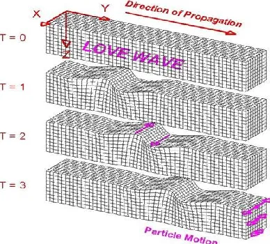
FIGURE 2: LOVE WAVE PROPAGATION ... 21

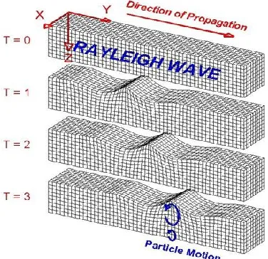
FIGURE 3: RAYLEIGH WAVE PROPAGATION ... 22

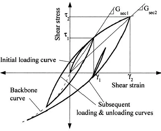
FIGURE 4: CYCLIC STRESS-STRAIN CURVE ... 23

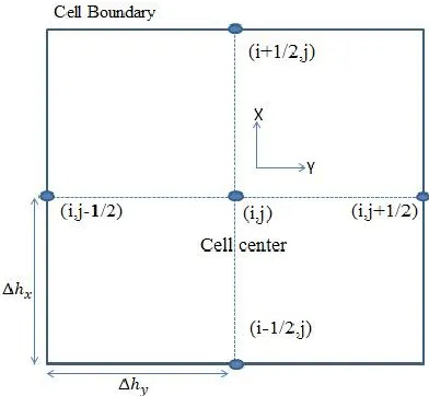
FIGURE 5: SCHEMATIC OF CELL USED IN THE FINITE VOLUME METHOD MESH ... 29

FIGURE 6: PROPAGATION OF FLUXES TO THE CELL BOUNDARIES SCHEMATIC REPRESENTATION ... 31

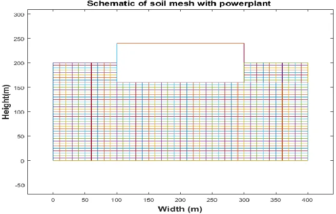
FIGURE 7: MESH OF THE SOIL AND THE POWER-PLANT STRUCTURE ... 32

FIGURE 8: 1D CASE-VELOCITY VS TIME AND NORMAL STRESS VS TIME PLOT... 36

FIGURE 9: 1D_ COMPARISON OF WAVEFORMS OF VELOCITY (U) AND NORMAL STRESS SIGMA VS DISTANCE TO SURFACE FOR MESH SIZE CONSIDERING 20(TOP), 50(MIDDLE), 100(BOTTOM) POINTS ... 37

FIGURE 10: 2D PURE SHEAR TEST_ COMPARISON OF WAVEFORMS OF VELOCITY (U) AND NORMAL STRESS SIGMA VS DISTANCE TO SURFACE FOR MESH SIZE CONSIDERING 10(TOP), 30(MIDDLE), 60(BOTTOM) POINTS ... 40

8 FIGURE 12: COMPARISON OF WAVEFORMS OF HORIZONTAL VELOCITY FOR MESH

SIZE CONSIDERING 10(TOP), 30(MIDDLE), 60(BOTTOM) POINTS ... 44

FIGURE 13: COMPARISON OF WAVEFORMS OF VERTICAL VELOCITY FOR MESH

SIZE CONSIDERING 10(TOP), 30(MIDDLE), 60(BOTTOM) POINTS ... 45

FIGURE 14: COMPARISON OF WAVEFORMS OF NORMAL STRESS IN X DIRECTION

FOR MESH SIZE CONSIDERING 10(TOP), 30(MIDDLE), 60(BOTTOM) POINTS ... 46

FIGURE 15: COMPARISON OF WAVEFORMS OF NORMAL STRESS IN Y DIRECTION

FOR MESH SIZE CONSIDERING 10(TOP), 30(MIDDLE), 60(BOTTOM) POINTS ... 47

FIGURE 16: COMPARISON OF WAVEFORMS OF SHEAR STRESS TAU FOR MESH SIZE

CONSIDERING 10(TOP), 30(MIDDLE), 60(BOTTOM) POINTS ... 48

FIGURE 17: COMPARISON OF WAVEFORMS OF VELOCITY/NORMAL STRESS IN X

DIRECTION AND SHEAR STRESS TAU VS DISTANCE FOR MESH SIZE

CONSIDERING 10(TOP), 30(MIDDLE), 60(BOTTOM) POINTS ... 49

FIGURE 18: GROUND ACCELERATION VS NUMBER OF POINTS IN X DIRECTION

(LEFT), GROUND VELOCITY VS TIME (RIGHT) ... 50

FIGURE 19: REAL DATA-COMPARISON OF WAVEFORMS OF HORIZONTAL

VELOCITY FOR MESH SIZE CONSIDERING 10(TOP), 30(MIDDLE), 60(BOTTOM)

POINTS ... 52

FIGURE 20: REAL DATA-COMPARISON OF WAVEFORMS OF VERTICAL VELOCITY

FOR MESH SIZE CONSIDERING 10(TOP), 30(MIDDLE), 60(BOTTOM) POINTS ... 53

FIGURE 21: REAL DATA-COMPARISON OF WAVEFORMS OF NORMAL STRESS IN X

DIRECTION FOR MESH SIZE CONSIDERING 10(TOP), 30(MIDDLE), 60(BOTTOM)

9 FIGURE 22: REAL DATA-COMPARISON OF WAVEFORMS OF NORMAL STRESS IN Y

DIRECTION FOR MESH SIZE CONSIDERING 10(TOP), 30(MIDDLE), 60(BOTTOM)

POINTS ... 55

FIGURE 23: REAL DATA-COMPARISON OF WAVEFORMS OF SHEAR STRESS TAU

FOR MESH SIZE CONSIDERING 10(TOP), 30(MIDDLE), 60(BOTTOM) POINTS ... 56

FIGURE 24: REAL DATA-COMPARISON OF WAVEFORMS OF VERTICAL VELOCITY/

NORMAL STRESS IN X DIRECTION/ SHEAR STRESS TAU FOR MESH SIZE

CONSIDERING 10(TOP), 30(MIDDLE), 60(BOTTOM) POINTS ... 57

FIGURE 25: REAL DATA-COMPARISON OF WAVEFORMS OF HORIZONTAL

VELOCITY FOR MESH SIZE CONSIDERING 10(TOP), 30(MIDDLE), 60(BOTTOM)

POINTS ... 60

FIGURE 26: REAL DATA MULTIPLE LAYERS-COMPARISON OF WAVEFORMS OF

VERTICAL VELOCITY FOR MESH SIZE CONSIDERING 10(TOP), 30(MIDDLE),

60(BOTTOM) POINTS ... 61

FIGURE 27:REAL DATA MULTIPLE LAYERS-COMPARISON OF WAVEFORMS OF

NORMAL STRESS SIGMA IN X DIRECTION FOR MESH SIZE CONSIDERING

10(TOP), 30(MIDDLE), 60(BOTTOM) POINTS ... 62

FIGURE 28: REAL DATA MULTIPLE LAYERS-COMPARISON OF WAVEFORMS OF

NORMAL STRESS SIGMA IN Y DIRECTION FOR MESH SIZE CONSIDERING

10(TOP), 30(MIDDLE), 60(BOTTOM) POINTS ... 63

FIGURE 29: REAL DATA MULTIPLE LAYERS-COMPARISON OF WAVEFORMS OF

SHEAR STRESS TAU FOR MESH SIZE CONSIDERING 10(TOP), 30(MIDDLE),

10 FIGURE 30: REAL DATA MULTIPLE LAYERS-COMPARISON OF WAVEFORMS OF

VERTICAL VELOCITY/NORMAL STRESS SIGMA IN X DIRECTION/SHEAR

STRESS TAU VS DISTANCE TO THE SURFACE FOR MESH SIZE CONSIDERING

10(TOP), 30(MIDDLE), 60(BOTTOM) POINTS ... 65

FIGURE 31: COMPARISON OF WAVEFORMS OF HORIZONTAL VELOCITY FOR A

MESH SIZE CONSIDERING 10(TOP) /30(MIDDLE) /60(BOTTOM) POINTS IN X AND

Y DIRECTION EACH ... 71

FIGURE 32: COMPARISON OF WAVEFORMS OF NORMAL STRESS IN X DIRECTION

FOR A MESH SIZE CONSIDERING 10(TOP) /30(MIDDLE) /60(BOTTOM) POINTS IN

X AND Y DIRECTION EACH ... 72

FIGURE 33: COMPARISON OF WAVEFORMS OF SHEAR STRESS TAU FOR A MESH

SIZE CONSIDERING 10(TOP) /30(MIDDLE) /60(BOTTOM) POINTS IN X AND Y

DIRECTION EACH ... 73

FIGURE 34: COMPARISON OF WAVEFORMS OF VERTICAL VELOCITY, NORMAL

STRESS IN X DIRECTION, SHEAR STRESS TAU FOR A MESH SIZE CONSIDERING

10(TOP) /30(MIDDLE) /60(BOTTOM) POINTS IN X AND Y DIRECTION EACH ... 74

FIGURE 35: SCHEMATIC OF A MONTE- CARLO SIMULATION. ... 77

FIGURE 36: HISTOGRAM AND SUPERIMPOSED PDFS FOR SAMPLE SIZE NRAND=100

... 78

FIGURE 37: HISTOGRAM AND SUPERIMPOSED PDFS FOR SAMPLE SIZE

NRAND=1000 ... 79

FIGURE 38: HISTOGRAM AND SUPERIMPOSED PDFS FOR SAMPLE SIZE

11

LIST OF TABLES

TABLE 1: SOIL PROPERTIES FOR DIFFERENT LAYERS ... 58

12

NOMENCLATURE

𝜎_𝑖𝑗 -stress tensor

𝜎𝑥, 𝜎𝑦 -normal stress in x and y respectively

𝜎̇ -derivative wrt time

𝜖_𝑖𝑗 -strain tensor

𝜖_𝑘𝑘 -sum of normal components of strain

𝛿_𝑖𝑗 -kronecker delta

𝜆, 𝜇 -lame parameters

𝛾 -shear strain

𝛾_𝑜𝑐𝑡 -octahedral strain

𝜏 -shear stress; also in 𝜏 ℎ𝑥,

𝜏

ℎ𝑦 it is the time step for FV scheme

𝜏_𝑚𝑎𝑥 -maximum shear stress

𝜏_𝑜𝑐𝑡 -octahedral stress G -shear modulus

𝐺𝑚𝑎𝑥 -maximum shear modulus

𝐸 -modulus of elasticity

𝐸̅ -modified modulus of elasticity

𝜌 -density

U -Velocity in x direction

V -Velocity in y direction

𝑢_𝑥 -partial derivative of u wrt x

13

𝜈 -poisons ratio C -p-wave velocity

𝐶_𝑔 - shear wave velocity W -Riemann invariants

14

1.

PROBLEM INTRODUCTION

On March 11th 2011, a tsunami caused by a gigantic earthquake hit the Tohoku Region pacific

coast in Northern Japan. The seismic center was estimated to be about 130 kilometers east of the

Oshika Peninsula of Tohoku, and 24 km underneath the seabed. It extended 500 km along the

coastline with a width of 200 km. The intensity of the earthquake was 9.0 on the Richter scale,

making it the fourth-largest earthquake recorded since 1900. The earthquake created a gigantic

tsunami wave that was about 10 m high at maximum. Once it reached land, it ran up to 40 m

above the sea level and intruded 6 km inland, causing catastrophic damage to many people and

towns along the coastline. About twenty thousand people lost their lives or are still missing, the

major cause of their death being by drowning. And while it is commonly known that several

nuclear power plants were lost, the reduction in electrical generating capacity due to the loss of

fossil power plants was actually larger.[1]

Presented example is the most destructive and disruptive seismic phenomena occurred recently.

Every day there are about fifty earthquakes worldwide that are strong enough to be felt locally

and every few days an earthquake occurs that is capable of damaging structures. In countries

where the earthquake resistant structural design has been enforced, earthquake fatalities have

decreased dramatically. Seismic design of engineering structures is based on the following

engineering disciplines:

- Engineering Seismology, dealing with the measurement prediction and characterization

of ground motions; with account to the site effects

- Geotechnical Engineering, studying nonlinear soil behavior and site response under

15 Although the earthquake did not directly cause structural damage to the power plant but it is

important to be prepared for such disasters. The work presented in this thesis aims at predicting

the waveforms of acceleration, velocity and stresses at a point on the surface and analyzing based

on seismogram data located at a certain distance from the point. This data can be used further by

structural/civil engineers to predict the damage that can be caused to a structure and ways to

16

2. LITERATURE

2.1 Related Vocabulary

Earthquake: Shaking or trembling of the earth that accompanies rock movements

extending anywhere from the crust to 680 km below the Earth’s surface. It is the release of stored

elastic energy caused by sudden fracture and movement of rocks inside the Earth. Part of the

energy released produces seismic waves, like P, S, and surface waves that travel outward in all

directions from the point of initial rupture. These waves shake the ground as they pass by. An

earthquake is felt if the shaking is strong enough to cause ground accelerations exceeding

approximately 1.0 cm/s2.

Epicenter:The point on the Earth’s surface directly above the focus of an earthquake.

Fault: A fracture or zone of fractures in rock along which the two sides have been

displaced relative to each other. If the main sense of movement on the fault plane is up

(compressional; reverse) or down (extensional; normal), it is called a dip-slip fault. Where the

main sense of slip is horizontal the fault is known as a strike-slip fault. Oblique-slip faults have

both strike and dip slip.

Fault plane: The plane along which the break or shear of a fault occurs. It is a plane of

differential movement, that can be vertical as in a strike slip fault or inclined like a subduction

zone fault.

Fault zone: Since faults do not usually consist of a single, clean fracture, the term fault

zone is used when referring to the zone of complex deformation that is associated with the fault

plane.

Focus: The point on the fault at which the first movement or break occurred, directly

17 Locked fault: A fault that is not slipping because frictional resistance on the fault is

greater than the shear stress across the fault (it is stuck). Such faults may store strain for extended

periods that is eventually released in an earthquake when frictional resistance is overcome.

Seismicity: The geographic and historical distribution (the “where?” and “how often?”)

of earthquakes.

Tectonics: Large-scale deformation of the outer part of the Earth resulting from forces in the Earth.

2.2 Seismic hazards

Any naturally occurring event such as earthquake, tornado, hurricane and floods which is

capable of causing deaths, injuries and property damage is termed as natural hazards. Out of

these, the hazards associated with earthquakes are termed as SEISMIC HAZARDS. Following

are the most important seismic hazards that frequently occur:

Ground Shaking

When an earthquake occurs, seismic waves radiate from the source and rapidly travel in all

directions through the earth’s crust. When these waves reach the ground surface, they produce

shaking that lasts few seconds or few minutes in severe cases. The strength and duration depends

on various factors such as characteristics of soil, intensity of earthquake, depth of the hypocenter.

Structural Hazards

This type of hazard usually is the one that comes to mind when one thinks of earthquakes.

Structural damage is the leading cause of death and loss to economy in many earthquakes.

Falling objects such as brick facings and parapets on the outside of a structure or heavy pictures

and shelves within a structure have caused casualties in many earthquakes. Interior facilities such

18 Liquefaction

This type of hazard occurs when soils lose their strength and appear to flow as fluids. The

soil loses the strength to support structures or remain stable. Since it occurs only in saturated

soils, liquefaction is most commonly observed near rivers, bays and water bodies.

Landslides

Strong earthquakes often cause landslides. More often, earthquake induced landslides cause

damage by destroying buildings or disrupting bridges and other constructed facilities. Many of

the landslides induced by earthquakes often occur due to liquefaction but many simply represent

the failures of slopes that were marginally stable under static conditions.

Tsunami and Seiche

Rapid vertical seafloor movements caused by fault rupture during earthquakes can produce

long-period sea waves called tsunamis. Tsunamis travel great distances at high speeds but are

difficult to detect since they usually have less heights (1m) and large wavelength at the point of

generation. As the wave approaches the shore the depth of the sea reduces and so does the speed

of the wave, increasing its height to several times the original height. Sometimes, the shape of

the sea floor in the coastal areas can amplify the wave, producing a nearly vertical wall of water

that rushes far inland and causing devastating damage.

Earthquake induced waves in enclosed bodies of water are called seiches. Typically they are

caused by long period seismic waves that match the natural period of oscillation of the water in a

lake or a reservoir. Another type of seiche can be formed when faulting causes permanent

19

2.3 Physics of Seismology

Seismic Waves

When an earthquake occurs, different types of seismic waves are produced: body waves and

surface waves. Body waves, which travel through the interior of the earth, are of two types:

P-waves and S-waves. Surface waves are of two types: Rayleigh wave and Love wave.

Body Waves

It has been generally accepted that the major part of the ground shaking during an earthquake is

due to the upward propagation of body waves from an underlying rock formation. Although

surface waves are also involved, their effects are generally considered of secondary

importance.[3]

P-Waves

Also known as primary waves/compressional waves/longitudinal waves, involve successive

compression and rarefaction of the materials through which they pass. They are analogous to

sound waves and the motion of individual particle is parallel to the direction of travel. Like

sound waves p-waves can travel through solids and fluids. These types of waves are the first

20 Figure 1: Displacements due to P-wave (top) and S-wave (bottom). P-wave results in a volume change and shearing in the

material through which they pass, whereas due to S-waves there is pure shear.

S-waves

Also known as shear waves/secondary waves/transverse waves, cause shearing deformation

as they travel through the material. The motion of individual particle is perpendicular to the

direction of wave travel. The direction of particle movement can be used to classify the

s-waves further into two types: SV-wave (vertical) and SH-wave (horizontal). Since the

S-waves cause shearing of the material through which they travel they cannot pass through

fluids since fluids cannot resist shear forces. waves are the most damaging to structures.

S-waves are the second to be recorded on a seismogram with a velocity of around 3km/s.

Surface waves

Travelling only through the crust, surface waves are of a lower frequency than body waves,

and are easily distinguished on a seismogram as a result. Though they arrive after body

waves, it is surface waves that are almost entirely responsible for the damage and destruction

associated with earthquakes. This damage and the strength of the surface waves are reduced

21 Love waves

It's the fastest surface wave and moves the ground from side-to-side. Confined to the surface

of the crust, Love waves produce entirely horizontal motion. The velocity is in the range of

2-4.4 km/s in the earth’s crust. These waves are typically faster than Rayleigh waves. The

motion of the waves is in both directions i.e. perpendicular to direction of propagation and

parallel to the earth’s surface.

Figure 2: Love wave propagation

Rayleigh waves

A Rayleigh wave rolls along the ground just like a wave rolls across a lake or an ocean. Because it

rolls, it moves the ground up and down and side-to-side in the same direction that the wave is

moving. Most of the shaking felt from an earthquake is due to the Rayleigh wave, which can be much

larger than the other waves. The velocity is in the range of 2-4.2 km/s. The motion is in both the

directions i.e. in the direction of wave propagation and perpendicular to the direction of wave

22 Figure 3: Rayleigh wave propagation

2.4 Soil behavior

Although the majority of publications consider soil as linear elastic medium, the stress-strain

curve obtained in a laboratory on a soil sample is a typical constitutive elastic – plastic nonlinear

curve. In the (𝜏, 𝛾) plane the behavior is characterized by a hysteresis loop, the surface and

23 Figure 4: Cyclic stress-strain curve

Strain amplitudes induced by major earthquakes are capable of creating significant

non-linearity’s and possibly irrecoverable deformations. The curve is explained by four rules called

the masing models. For initial loading the soil follows the loading curve along the backbone

curve. At the point of stress reversal or unloading (in the above picture corresponding to stress

𝜏₁) the path followed is similar in shape to the backbone curve but that of unloading and

displaced by a certain shear strain which is called the residual shear strain. It follows the shape

until it intersects the backbone curve after which it follows it until a point of loading. This is

followed for the number of loading and unloading cycles.[2] This behavior is called the

hysteretic behavior of soil. In our case we have used the hyperbolic backbone curve equation

proposed by Arefi et al, 2012,[4] which is expressed as

𝜏 = 𝐺𝑚𝑎𝑥𝛾

1+𝛽|𝐺𝑚𝑎𝑥 𝜏𝑚𝑎𝑥𝛾|

24

3. OBJECTIVES

1) To develop a linear 2D seismic wave propagation computer model in a time-space domain

characterized by constant and variable ground properties using MATLAB.

2) To verify the accuracy of a model by comparing results with harmonic load data.

3) To develop a nonlinear 2D seismic wave propagation computer model in a time-space domain

incorporating nonlinear effective stress based soil model.

4) To develop a stochastic counterpart of created deterministic model that accounts for

25

4. LINEAR MODEL DEVELOPMENT

4.1 Governing equations of complete 3D system

It is assumed that the solid is a homogeneous isotropic material. The motion for the elastic

medium can be expressed as (with Einstein summation convention), [5]

𝜌𝜕2𝑢𝑖 𝜕𝑡2 =

𝜕𝜎𝑖𝑗

𝜕𝑥𝑗 + 𝜌𝑓𝑖, 𝑥 ∈ Ω, 𝑡 > 0, 𝑖 = 1,2,3

(2)

Where 𝜌 is the density of the material (taken to be constant), 𝑓𝑖 are components of acceleration due to an applied body force, and the components of stress are given by:

𝜎_𝑖𝑗 = 𝜆(𝜖_𝑘𝑘)𝛿_𝑖𝑗 + 2𝜇𝜖_𝑖𝑗, 𝜖_𝑖𝑗 = 1

2( 𝜕𝑢𝑖 𝜕𝑥𝑗+

𝜕𝑢𝑗

𝜕𝑥𝑖)(general theory of elasticity)

(3)

Here, 𝜖_𝑖𝑗and 𝛿_𝑖𝑗 are the components of the (linear) strain tensor and the identity tensor, respectively, 𝜖_𝑘𝑘 = ∑ 𝜖_{𝑘 𝑘𝑘} = ∇. 𝑢 is the divergence of the displacement, and 𝜆 and 𝜇 are Lame

parameters. The latter are related to Young’s Modulus E and Poisson’s ratio 𝜈 by

𝜇 =

2(1+𝜈)

and 𝜆 = 𝜈𝐸/((1 + 𝜈)(1 − 2𝜈)). Initial conditions for the second-order system in (2) are

𝑢(𝑥, 0) = 𝑢₀(𝑥),𝜕𝑢

𝜕𝑡(𝑥, 0) = 𝑣0(𝑥), 𝑥 ∈ Ω,

(4)

In our work we formulate the governing equations as a first order hyperbolic system in a

conservative form.

𝜕𝑢𝑖 𝜕𝑡 = 𝑣𝑖, 𝜕𝑣𝑖

𝜕𝑡 = 1 𝜌(

𝜕𝜎𝑖𝑗 𝜕𝑥𝑗) + 𝑓𝑖, 𝜕𝜎𝑖𝑗

𝜕𝑡 = 𝜆(𝜖̇𝑘𝑘)𝛿𝑖𝑗 + 2𝜇𝜖̇𝑖𝑗}

𝑥 ∈ Ω, 𝑡 > 0, 𝑖 = 1,2 … … 𝑛𝑑,

(5)

26

𝜖̇𝑖𝑗 = 1 2( 𝜕𝑣𝑖 𝜕𝑥𝑗+ 𝜕𝑣𝑗 𝜕𝑥𝑖) (6)

Initial conditions for displacement and velocity are given by u0(x) and v0(x) as before, and initial

conditions for the components of stress may be derived from (2) applied at t=0. Note that

contrary to what is typically done, we retain the displacements in our formulation of the first

order system. Retaining the displacements in the formulation allows the stress-strain relationship

(2) to be explicitly imposed at the boundary. In addition it will be useful to have the

displacement field when solving fluid-structure interaction problems (to define the fluid-solid

interface for grid generation, for example).

The governing equations, whether written as second-order or first-order system, are hyperbolic

and represent the motion of elastic waves in the solid. For the second order system, the

characteristic wave speeds for a homogeneous material in a periodic or infinite space are +-Cp

and +-Cs, where the pressure and shear wave speeds are given by 𝑐𝑝 = √ 𝜆+2𝜇

𝜌 and 𝑐𝑠 = √ 𝜇 𝜌,

Nevertheless formulation (5) seems to be more appropriate, as it allows the use of

well-developed mathematical tools for studying various wave propagating boundary value problems

based on characteristics theory. Elastic wave propagation measurements in a laboratory

experimental model and a field test site have shown similar propagation characteristics despite

widely different soil compositions and environmental conditions.[6]

For linear elastic model we apply the same procedure that was introduced for scalar waves to

vector wave scattering by a localized elastic inhomogeneity (e.g. Knopoff and Hudson 1964;

Miles 1960; Sato 1984 a, b, 1990; Wu 1989; Wu and Aki 1985).

Applying stochastic analysis the spatial variations in Lame’ coefficients and mass density are

27

𝜆(𝑥) = 𝜆₀+ 𝛿𝜆(𝑥), 𝜇(𝑥) = 𝜇₀+ 𝛿𝜇(𝑥) 𝑎𝑛𝑑 𝜌(𝑥) = 𝜌₀+ 𝛿𝜌(𝑥). (7)

Where variations of Lame’ parameters and density are modeling as normal or lognormal

distributions with a zero mean value. Equations (5) become PDE equations with random

coefficients. Numerical modelling is a useful tool to understand the role of different parameters

28

4.2 Augmented 2-dimensional system in Cartesian coordinates

In the two dimensional case, complete set of equations (5) can be reduced to five equations (8) –

(12)

𝜎𝑥̇ =𝐸̅(𝑢𝑥+ 𝜗𝑣𝑦) (8)

𝜎̇_𝑦 = 𝐸̅(𝑣_𝑦+ 𝜗𝑢_𝑥) (9)

𝜏̇ = 𝐺(𝑢_𝑦+ 𝑣_𝑥) (10)

𝑢̇ = 1

𝜌(𝜎𝑥,𝑥+ 𝜏𝑦) (11)

𝑣̇ =1

𝜌(𝜏𝑥+ 𝜎𝑦,𝑦) (12)

The following notations are used: u, v are velocity components, 𝜎𝑥, 𝜎𝑦, 𝜏 – two dimensional normal and shear stress components, dot above means time derivative, 𝐸, 𝐺, 𝜌 – tensile elastic constant, shear elastic constant and density of a soil accordingly, 𝐸̅ = 𝐸

1−𝜗2 is the modified elastic

constant. Partial derivative of an index free variable by an x or y coordinates is indicated by a

relating subscript, whereas for an indexed variable it is defined by the same comma separated

subscript.

We adopt the following augmented two-dimensional system in matrix form

𝑄̇ + 𝐴𝑄𝑥+ 𝐵𝑄𝑦 = 0 (13)

Where Q – is the vector of conservative variables, and A and B 5x5 matrices

𝑄 = ( 𝜎_𝑥 𝜎_𝑦 𝜏 𝑢 𝑣 ) A= [

0 0 0 𝐸 0 0 0 0 𝜈𝐸 0 0 0 0 0 𝐺 1/𝜌 0 0 0 0 0 0 1/𝜌 0 0]

B=

[

0 0 0 0 𝜈𝐸 0 0 0 0 𝐸 0 0 0 𝐺 0 0 0 1/𝜌 0 0 0 1/𝜌 0 0 0 ]

29

4.3 Eigen structure of the system

We analyze the Eigen structure of matrices A and B, using the MATLAB linear algebra toolbox.

The eigenvalues and eigenvectors of A are found to be

⋀𝑥 = 𝑑𝑖𝑎𝑔(0 𝑐 𝑐𝑔 − 𝑐 −𝑐𝑔) ; 𝑐 = √ 𝐸

𝜌;𝑐𝑔 = √ 𝐺 𝜌;

(14)

𝑊𝑥_{= [(𝜎}

𝑦− ν𝜎𝑥) 𝑢−𝜎𝑥_𝜌𝑐

2 𝑣− 𝜏

𝜌𝑐𝑔 2

𝑢+𝜎𝑥_𝜌𝑐

2 𝑣+ 𝜏

𝜌𝑐𝑔 2 ]

(15)

The Eigen structure of matrix B is characterized by the following vectors

⋀𝑦 = 𝑑𝑖𝑎𝑔(0 𝑐 𝑐_𝑔− 𝑐 −𝑐_𝑔); (16)

𝑊𝑦 _{= [𝜎}

𝑥− ν𝜎𝑦 𝑣−𝜎𝑦_𝜌𝑐

2 𝑢− 𝜏

𝜌𝑐𝑔 2

𝑣+𝜎𝑦_𝜌𝑐

2 𝑢+ 𝜏

𝜌𝑐𝑔 2 ]

(17)

4.4 Finite-volume numerical scheme

Consider now a control volume in x-y-t space of dimensions ℎ_𝑥 = 𝑥_𝑖+1/2− 𝑥_𝑖−1/2 ; ℎ_𝑦 = 𝑦𝑗+1/2− 𝑦𝑗−1/2, 𝜏 = 𝑡𝑛+1−𝑡𝑛, where fractional index relates to the cell edges, and the whole index – to the cell center.

30 A finite volume method for solving (13) reads

𝜎_{𝑥 𝑖,𝑗}𝑛+1 = 𝜎_{𝑥 𝑖,𝑗}𝑛 +E [𝜏

ℎ𝑥(𝑢𝑖+1₂,𝑗− 𝑢𝑖−1₂,𝑗) + 𝜗𝜏

ℎ𝑦 (𝑣𝑖,𝑗+1₂− 𝑣𝑖,𝑗−1₂)]

(18)

𝜎_{𝑦 𝑖,𝑗}𝑛+1 = 𝜎_{𝑦 𝑖,𝑗}𝑛 +E [𝜏𝜗 ℎ𝑥(𝑢𝑖+

1 2,𝑗

− 𝑢_𝑖−1 2,𝑗

) + 𝜏

ℎ𝑦(𝑣𝑖,𝑗+ 1 2

− 𝑣_𝑖,𝑗−1 2

)] (19)

𝜏_𝑖,𝑗𝑛+1 = 𝜏 _𝑖,𝑗𝑛 +G [𝜏

ℎ𝑥(𝑣𝑖+1₂,𝑗− 𝑣𝑖−1₂,𝑗) + 𝜏

ℎ𝑦(𝑢𝑖,𝑗+1₂− 𝑢𝑖,𝑗−1₂)]

(20)

𝑢_𝑖,𝑗𝑛+1 = 𝑢 _𝑖,𝑗𝑛 + 1 𝜌[

𝜏 ℎ𝑥(𝜎𝑥𝑖+

1 2,𝑗

− 𝜎_𝑥𝑖−1 2,𝑗

) + 𝜏

ℎ𝑦(𝜏𝑖,𝑗+ 1 2

− 𝜏_𝑖,𝑗−1 2

)] (21)

𝑣_𝑖,𝑗𝑛+1 = 𝑢 _𝑖,𝑗𝑛 + 1 𝜌[

𝜏 ℎ𝑥(𝜏𝑖+1

2,𝑗

− 𝜏_𝑖−1 2,𝑗

) + 𝜏

ℎ𝑦(𝜎𝑦 𝑖,𝑗+1 2

− 𝜎_{𝑦 𝑖,𝑗−}1 2

)] (22)

The description of scheme (18)-(22) is complete once expressions for the numerical fluxes

relating to the cell edges are provided. Godunov [9] proposed to use the self - similar solution of

the Riemann problem to compute numerical fluxes in the direction normal to the cell faces, the

algorithm which forms the foundation of a contemporary TVD (total variation diminishing)

family of methods, applicable to model propagation of waves of a different physical nature.[10]

The numerical procedure is time marching, monotone, implicit, of second order accuracy by

space and time coordinates.[11]

Below we present the algorithm of calculating a few of flux terms based on a centered cell values

𝑢_𝑖+1 2,𝑗

= 𝑊₂𝑥_𝑖𝑗 + 𝑊₄𝑥

𝑖+1,𝑗 (23)

𝜎_𝑥𝑖+1 2,𝑗

= 𝜌𝑐(−𝑊₂𝑥_𝑖𝑗+ 𝑊₄𝑥_𝑖+1,𝑗) (24)

𝑣_𝑖+1 2,𝑗

= 𝑊₃𝑥_𝑖𝑗+ 𝑊₅𝑥_𝑖+1,𝑗 (25)

𝜏_𝑖+1 2,𝑗

31

4.5 Solution propagation

Figure 6: Propagation of fluxes to the cell boundaries schematic representation

The above figure represents how the flux propagates to the cell boundaries and the advance of

the solution. In the previous section we presented the transformation of the problem to

Riemann[12] invariants with fluxes at the boundaries related to fractional indices and properties

at cell centers related by whole indices. At any time instant the properties at the cell centers are

dependent on the properties of the cell at the previous instant of time and the fluxes along the

boundaries of the cells. They are related by the expressions in equation (18)-(22). The Riemann

variable presented in equation (15) and (17) has the characteristic speed ±𝐶 𝑎𝑛𝑑 ± 𝐶_𝑔 where g represents the shear wave speed. These variables propagate with positive speeds in the positive

direction and similarly in the negative direction. The characteristics carry the information to the

cell boundaries where the fluxes with fractional indices are calculated. The domain of the

problem is accounted for in the finite-volume approach. This ensures the satisfaction of the

physical law over the finite region rather than at a point. The discretization has the quality to

conserve the properties over the finite space. [13]

For example,

𝑊𝑥4(𝑖, 𝑗) = 𝑊𝑥4(𝑖, 𝑗 + 1 2)=

1

2(𝑢𝑖,𝑗+1₂+ 1

𝜌𝑐𝜎𝑥,𝑖,𝑗+1₂) ,

𝑊_𝑥2(𝑖, 𝑗 + 1)=𝑊_𝑥2(𝑖, 𝑗 +1

2)= 1

2(𝑢𝑖,𝑗+1₂− 1

32 Similarly the process repeats for every cell and every property that is normal stress, shear stress and velocities in X and Y directions.

Figure 7: Mesh of the soil and the power-plant structure

4.6 Boundary conditions

(1) Downward

At the depth, the kinematic boundary conditions identify relating flux components as the

measured components of velocities

𝑢_𝑖=1 2,𝑗

= 𝑢₀(𝑡, 𝑦) (27)

𝑣_𝑖=1 2,𝑗

= 𝑣0(𝑡, 𝑦) (28)

Relating stress components are calculated based on a similarity solution for x – propagating

invariants

𝑊𝑥4(𝑖 = 1, 𝑗) = 𝑊𝑥4(𝑖 = 1

2, 𝑗) = (𝑢𝑖=1₂,𝑗+ 1

𝜌𝑐𝜎𝑥,𝑖=1₂,𝑗) 1 2

33

𝜎_𝑥,𝑖=1 2,𝑗

= 𝜌𝑐(2𝑊_𝑥4,𝑖=1 2,𝑗=1

− 𝑢_𝑖=1 2,𝑗

) (30)

𝑊_𝑥5(𝑖 = 1, 𝑗) = 𝑊_𝑥5(𝑖 = 1

2, 𝑗) = (𝑣𝑖=1 2,𝑗

+ 1

𝜌𝑐𝜏𝑖=1 2,𝑗

)1

2

(31)

𝜏_𝑖=1 2,𝑗

= 𝜌𝑐(2𝑊_{𝑥5,𝑖=1,𝑗}− 𝑣_𝑖=1 2,𝑗

) (32)

(2) Free Surface

At the free surface the normal and tangential stress components are assumed to be equal to zero.

This is in accordance with the study by Maria Paola Santisi d’ Avila and Jean-Francois

Semblat.[14]

𝜎_{𝑥,𝑁𝑥+}1 2,𝑗

= 0 (33)

𝜏_{𝑥,𝑁𝑥+}1 2,𝑗

= 0 (34)

Relating velocity components are calculated based on x – propagating invariants

𝑊𝑥2.𝑖=𝑁𝑥,𝑗 = 1

2(𝑢𝑁𝑥+1₂,𝑗− 1

𝜌𝑐𝜎𝑥,𝑁𝑥+1₂,𝑗) (35)

𝑢_𝑁𝑥+1 2,𝑗

= 2𝑊_{𝑥2.𝑖=𝑁𝑥,𝑗} (36)

𝑊_{𝑥3.𝑖=𝑁𝑥,𝑗} =1

2(𝑣 − 𝜏 𝜌𝑐𝑔)𝑁𝑥+

1 2,𝑗

(37)

𝑣_𝑁𝑥+1 2,𝑗

= 2𝑊_{𝑥3,𝑁𝑥,𝑗} (38)

(3) Left Boundary Condition

Non-reflected (absorbed) boundary conditions are implemented, which means that the reflected

(right invariants) are equal to zero. These conditions are supplemented by the left invariants

34

𝑊_𝑦2,𝑗=1 2

= (𝑣 −𝜎𝑦

𝜌𝑐)_𝑖,𝑗=1 2

.1

2= 0 ; 𝑣𝑖,𝑗=1₂ = 𝑊𝑦4,𝑖,𝑗=1₂; (39)

𝑊_𝑦4,𝑗=1 2

= (𝑣 +𝜎𝑦

𝜌𝑐)_𝑖,𝑗=1 2

.1

2 ; 𝜎𝑦,𝑖,𝑗=1 2

= 𝜌𝑐. 𝑣_𝑖,𝑗=1 2

; (40)

𝑊_{𝑦3,𝑖,𝑗=}1 2

= (𝑢 − 𝜏

𝜌𝑐𝑔)_𝑖,𝑗=1 2

.1

2 = 0

(41)

𝑊_{𝑦5,𝑖,𝑗=}1 2

= (𝑢 + 𝜏

𝜌𝑐𝑔)_𝑖,𝑗. 1 2

(42)

𝑢_𝑖,1 2

= 𝑊_{𝑦5,𝑖,𝑗=1}; 𝜏 = 𝜌𝑐_𝑔𝑢_𝑖,𝑗=1 2

(43)

(4) Right Boundary conditions

Non-reflected (absorbed) boundary conditions are implemented, which means that the reflected

(left invariants) are equal to zero. These conditions are supplemented by the right invariants

arriving to the right boundary

𝑊_{𝑦4,𝑖,𝑗=𝑁𝑦+}1 2

= (𝑣 +𝜎𝑦

𝜌𝑐)_{𝑖,𝑗=𝑁𝑦+}1 2

.1

2

(44)

𝑊_{𝑦2,𝑖,𝑗=𝑁𝑦+}1 2

= (𝑣 −𝜎𝑦

𝜌𝑐)_{𝑖,𝑗=𝑁𝑦+}1 2

.1

2

(45)

𝑣_{𝑖,𝑁𝑦+}1 2

= 𝑊_{𝑦2,𝑖,𝑗=𝑁𝑦} ; 𝜎_𝑦 = −𝜌𝑐𝑣_{𝑖,𝑁𝑦+}1 2

; (46)

𝑊_{𝑦5,𝑖,𝑗=𝑁𝑦+}1 2

= (𝑢 + 𝜏

𝜌𝑐𝑔)_{𝑖,𝑗=𝑁𝑦+}1 2

.1

2=0

(47)

𝑊_{𝑦3,𝑖,𝑗=𝑁𝑦+}1 2

= (𝑢 − 𝜏

𝜌𝑐𝑔)_{𝑖,𝑗=𝑁𝑦+}1 2

.1

2

(48)

𝑢_{𝑖,𝑁𝑦+}1 2

= 𝑊𝑦3,𝑖,𝑗=𝑁𝑦 ; 𝜎𝑦 = −𝜌𝑐𝑦𝑢_{𝑖,𝑁𝑦+}1 2

35

4.7 1D testing case

Assume that deformation of the medium is one-dimensional, and only one axial component of

the stress tensor and velocity vector is nonzero. The physical and numerical models are

described by equations (8), (11) and (18), (21) accordingly. We run the scheme (18), (21) with

the following input data:

The total length L=200m; density 𝜌=2000kg/m^3; time of simulation T=5s; speed of pressure waves propagation c=1636𝑚/𝑠; frequency of a propagating wave 𝜔 =𝜋𝐿

𝑐 ; Courant-Friedrichs-Lewy number cfl=0.5. It simply states that the method must be used in such a way that

information has a chance to propagate at the correct physical speeds, as determined by the

eigenvalues of the flux.[10] The linear elastic Young modulus was calculated based on a speed

of sound and density 𝐸 = 𝜌𝑐2.

An exact solution for the one-dimensional case was adopted in a form

𝑈(𝑥, 𝑡) = sin (𝜋𝑥

𝐿) sin(𝜔𝑡) ;

𝜎(𝑥, 𝑡) = −𝜌𝑐 ∗ 𝑐𝑜𝑠 (𝜋𝑥

𝐿) cos(𝜔𝑡);

Boundary conditions, compliant with the exact solution are:

𝑈(0, 𝑡) = 0; 𝜎(𝐿, 𝑡) = 𝜌𝑐 cos(𝜔𝑡).

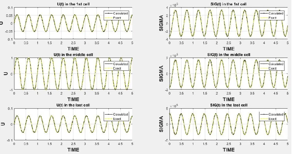
We ran simulations with three different meshes of 20, 50 and 100 cells. Figure 9 presents time

dependent distributions of velocity (left) and normal stress (right) at the first, middle and the last

cells. The plots of exact and numerical solutions are non-distinguishable for all three numerical

36 Figure 8: 1D case-Velocity vs Time and Normal Stress vs Time plot

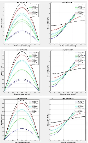
The snapshots of velocity and normal stress waveforms are presented in Figure.9 for three

different meshes at five instances of time: T/5, 2T/5, 3T/5, 4T/5, T for numerical (dash lines) and

exact solutions (solid lines). It appears that space numerical distributions are more sensitive to

the cell count, matching exact solution (lines non-distinguishable) for the 100 cells at cfl=0.5. It

should be noted that cfl =1 results in much more accurate results, but we intentionally use

37 Figure 9: 1D_ Comparison of waveforms of Velocity (U) and normal Stress sigma vs Distance to surface for mesh size

38

4.8 2D pure shear dynamic deformation test

Assume that deformation of the medium is two-dimensional, and only one component of a stress

tensor – shear stress, and both components of a velocity vector are nonzero. The physical and

numerical models are described by equations (10) - (12) and (20) - (22) accordingly. We run the

scheme (20), (21), (22) with the following input data:

The total length of the area L=400m; depth H=400m; density p=2000𝑘𝑔/𝑚3; time of simulation T=100s; speed of pressure waves propagation c=1636𝑚/𝑠; Poisson coefficient 𝜗 = 0.4 ; Shear wave propagation velocity was calculated based on a Poisson correction 𝑐_𝑔 = 𝑐

𝑠𝑞𝑟𝑡(𝐸(1+𝜗)); Frequency of a propagating wave 𝜔 =𝜋𝐿

𝑐 ; Courant-Friedrichs-Lewy number cfl=0.5. The linear elastic and shear moduli have been calculated based on relating velocities of sound and

density 𝐸 = 𝜌𝑐2_{, 𝐺 = 𝜌𝑐} 𝑔2.

An exact solution for the one-dimensional case was adopted in a form

𝑈(𝑥, 𝑦, 𝑡) = cos (𝜋𝑥

𝐻) sin ( 𝜋𝑦

𝐿) cos(𝜔𝑡) ;

(50)

𝑉(𝑥, 𝑦, 𝑡) = sin (𝜋𝑥

𝐿) cos ( 𝜋𝑦

𝐿) cos(𝜔𝑡);

(51)

𝜏(𝑥, 𝑦, 𝑡) =2𝐺

𝜔 𝜋 𝐿cos (

𝜋𝑥 𝐿) cos (

𝜋𝑦

𝐿 ) 𝑠𝑖𝑛(𝜔𝑡);

(52)

Boundary conditions, compliant with the exact solution are:

𝑉(0, 𝑦, 𝑡) = 0; 𝜏(𝐿, 𝑦, 𝑡) = −2𝐺

𝜔 𝜋 𝐿cos (

𝜋𝑦

𝐿 ) 𝑠𝑖𝑛(𝜔𝑡)

(53)

𝑈(𝑥, 0, 𝑡) = 0; 𝜏(𝑥, 𝐿, 𝑡) = −2𝐺

𝜔 𝜋 𝐿cos (

𝜋𝑥

𝐿) 𝑠𝑖𝑛(𝜔𝑡)

(54)

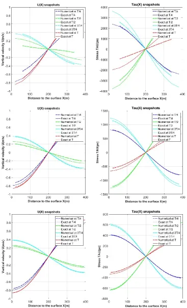
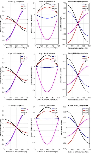
39 T. Numerical solution relating to cfl=0.5 is presented by dash lines, and exact solutions by solid

lines. Evidently, that the finest mesh provides the better match. Similar to the one –dimensional

case, application of cfl =1 results in much more accurate results, but we intentionally use cfl=0.5,

which provides an extra stability margin for the nonlinear cases. Additional plots, including

40 Figure 10: 2D pure shear test_ Comparison of waveforms of Velocity (U) and normal Stress sigma vs Distance to surface for

41 Figure 11: 2D pure shear test_ Comparison of waveforms of vertical velocity, horizontal velocity, shear stress vs Distance to

42

4.9 2D harmonic load constant properties

The physical and numerical models are described by equations (8) - (12) and (18) - (22)

accordingly. We ran the scheme (18)-(22) with the following input data:

The total length of the area L=400m; depth H=200m; density 𝜌 = 2000𝑘𝑔/𝑚3; time of simulation T=10s; speed of pressure waves propagation 𝑐 = 1636𝑚/𝑠; Poisson coefficient

𝜈 = 0.4 ; Shear wave propagation velocity was calculated based on a Poisson correction

𝑐𝑔 = 𝑐

𝑠𝑞𝑟𝑡(𝐸(1+𝜈)); Courant-Friedrichs-Lewy number CFL=0.5. The linear elastic and shear moduli have been calculated based on relating velocities of sound and density 𝐸 = 𝜌𝑐2, 𝐺 =

𝜌𝑐_𝑔2_{. A stability criterion prescribes the “safe” time step as Δ𝑡 =} 𝐶𝐹𝐿 𝑐(1

ℎ𝑥+ 1 ℎ𝑦)

. Three types of meshes

have been employed: 10x10, 30x30 and 60x60 cells. To prove monotonicity of a numerical

scheme the artificial acceleration load in a y-direction has been approximated as a harmonic

function ACCELY=0.2𝜋 ∗4

𝑇cos ( 4𝜋𝑡

𝑇 ) sin ( 𝜋𝑦

𝐿). Since boundary conditions in our model should be specified in a form of either velocity or the stress tensor components, acceleration function

was integrated to obtain velocity profile VELY=0.2 sin (4𝜋𝑡

𝑇 ) sin ( 𝜋𝑦

𝐿). In addition we applied the x – component of velocity assuming that the angle between the wave front and the horizontal

direction is 6o, so that VELX=VELY*tan (6o). Multiple results of parametric analysis on

different meshes are presented in Figures 12 – 17. In this case we do not have an exact solution,

but we can check the monotonicity, coherence, boundary condition satisfaction, convergence.

Figure 12 and 13 present the time distribution of horizontal and vertical components of velocities

accordingly. Each figure contains nine subplots, relating to the mesh 10x10 (upper line), 30x30

43 point, indicated by legend, inside calculation domain. All distributions are monotone and

coherent. Figures 12-16 present time evolution of three stress components, calculated at the same

characteristic points, using the same three computational meshes. It is easy to see that the x

component of normal stress and a shear stress component tend to zero approaching the ground

surface. The small deviation from zero is explained by the fact that the stress components in our

algorithm relate to the cell centers, whereas boundary conditions are applied to the cell side.

The last Figure 17 visualizes the snapshots of the velocity component, normal stress in

x-direction and a shear stress component. All components are monotone, and satisfy to the applied

boundary conditions at the free surface, where the normal stress and shear stress should be

absent, and applied conditions at the depth where both components of velocities are specified.

Convergence on a sequence of meshes is observed based on a fact that the boundary conditions

44

46 Figure 14: Comparison of waveforms of normal stress in X direction for mesh size considering 10(top), 30(middle),

47 Figure 15: Comparison of waveforms of normal stress in Y direction for mesh size considering 10(top), 30(middle),

49 Figure 17: Comparison of waveforms of velocity/normal stress in X direction and shear stress TAU vs Distance for mesh size

50

4.10 2D real load constant properties

The physical and numerical models are described by equations (8) - (12) and (18) - (22)

accordingly. We ran the scheme (18)-(22) with the input data described in the previous section.

For the present case the real acceleration profile applied at the depth of 200 m is used. Black

indicates all 4000 input data points, whereas red color profile corresponds to the uniformly

distributed 400 input point (Figure 18, left). Figure 18, right describes distribution of

velocity𝑉𝐸𝐿 = ∫ 𝐴𝐶𝐶𝐸𝐿(𝜏)𝑑𝜏₀𝑡 . The coarse mesh based distribution of input acceleration and velocity skip a large number of local peaks inherent for the fine mesh, which can result in a

notable inaccuracy.

Figure 18: Ground acceleration vs number of points in X direction (Left), Ground velocity vs Time (Right)

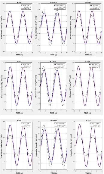
Multiple results of parametric analysis on different meshes are presented in Figures 20–25.

Figures 20 – 24 present time distributions of horizontal and vertical components of velocities,

and three components of a stress tensor accordingly. Each figure contains nine subplots, relating

51 corresponds to the selected characteristic point, indicated by legend, inside calculation domain.

All distributions are non-monotone since the input data is non-monotone. Figures 20-24 present

time evolution of three stress components, calculated at the same characteristic points, using the

same three computational meshes. It is again easy to see that the x component of normal stress

and a shear stress component tend to zero approaching the ground surface. The small deviation

from zero is explained by the fact that the stress components in our algorithm relate to the cell

centers, whereas boundary conditions are applied to the cell side.

The last Figure 25 visualizes the snapshots of all velocity and stress components. All

components satisfy to the applied boundary conditions at the free surface, where the normal

stress and shear stress should be equal to zero, and applied conditions at the depth where both

components of velocities are specified. Convergence on a sequence of meshes is observed based

52 Figure 19: Real Data-Comparison of waveforms of horizontal velocity for mesh size considering 10(top), 30(middle),

53 Figure 20: Real Data-Comparison of waveforms of vertical velocity for mesh size considering 10(top), 30(middle), 60(bottom)

54 Figure 21: Real Data-Comparison of waveforms of normal stress in X direction for mesh size considering 10(top), 30(middle),

55 Figure 22: Real Data-Comparison of waveforms of normal stress in Y direction for mesh size considering 10(top), 30(middle),

56 Figure 23: Real Data-Comparison of waveforms of shear stress TAU for mesh size considering 10(top), 30(middle), 60(bottom)

57 Figure 24: Real Data-Comparison of waveforms of vertical velocity/ normal stress in X direction/ shear stress TAU for mesh

58

4.11 2D real load multi layered linear soil structure

Among the most important effects of seismic waves is the strong dependence of damage on its

location, though the distance from different sites to the oncoming wave is the same. This

phenomenon is due to the variability of site local properties, which alter the characteristics of

seismic motion and cause concentrations of damage during earthquakes. There are two ways of

describing the sedimentary infilling properties: the basin is either composed of distinct

homogeneous geological layers or through properties progressively changing as a function of

depth.[8] We have used a similar model as the latter one by discretizing the soil into a system of

horizontal layers parallel to x-y plane except that the properties for different layers have been

assumed unlike a function of depth. Local site effects have an important effect on the surface

ground motion. The soil profile characteristics from the used site are presented inTable 1. These

are average properties taken from the Geophysical Journal International.[14]

Layer # Thickness (m) Mass density (kg/m3) Elastic modulus (MPa) Poisson ratio

1 20 2000 4.49*103 _0.4

2 30 2200 5.19*103 _0.4

3 50 2500 5.49*103 _0.4

4 100 2900 6.4*103 _0.4

Table 1: Soil properties for different layers

The rest of properties and a seismic load are identical to the ones presented in the previous

section.

The physical and numerical models are described by equations (8) - (12) and (18) - (22)

accordingly. The only difference in the algorithm applied to the multi layered structure is that

solution of the Riemann problem (23) – (26), relating to the cell flux, is generalized, becoming

59 Multiple results of parametric analysis on different meshes are presented in Figures 26–31.

Figures 26 – 27 present time distributions of horizontal and vertical components of velocities,

and three components of a stress tensor accordingly. Each figure contains nine subplots, relating

to the mesh 10x10 (upper line), 30x30 (middle line) and 60x60 (bottom line). Each subplot

corresponds to the selected characteristic point, indicated by legend, inside calculation domain.

All distributions are non-monotone since the input data is non-monotone. Figure 27, 28 and 29

present time evolution of three stress components, calculated at the same characteristic points,

using the same three computational meshes. We can see that the x component of normal stress

and a shear stress component tend to zero approaching the ground surface. The small deviation

from zero is explained by the fact that the stress components in our algorithm relate to the cell

centers, whereas boundary conditions are applied to the cell side.

The last Figure 30 visualizes the snapshots of all velocity and stress components. All

components satisfy to the applied boundary conditions at the free surface, where the normal

stress and shear stress should be equal to zero, and applied conditions at the depth where both

components of velocities are specified. Convergence on a sequence of meshes is observed based

60 Figure 25: Real Data-Comparison of waveforms of horizontal velocity for mesh size considering 10(top), 30(middle),

61 Figure 26: Real Data multiple layers-Comparison of waveforms of vertical velocity for mesh size considering 10(top),

62 Figure 27:Real Data multiple layers-Comparison of waveforms of normal stress SIGMA in X direction for mesh size

63 Figure 28: Real Data multiple layers-Comparison of waveforms of normal stress SIGMA in Y direction for mesh size

64 Figure 29: Real Data multiple layers-Comparison of waveforms of shear stress TAU for mesh size considering 10(top),

65 Figure 30: Real Data multiple layers-Comparison of waveforms of vertical velocity/normal stress SIGMA in X direction/shear

66

4.12 2D nonlinear properties seismic ground motion wave

propagation

It is obvious that soil does not react elastically. Contrary to the conventional modeling, which

assumes linear elastic behavior of the soil, the present approach uses an elastic-plastic model

reproducing a variety of experimentally observed hysteretic soil behavior. Structures which are

located in areas where large nonlinear behavior of soil is observed face not only horizontal and

vertical components of inertial forces by earthquake shaking but can also experience large

differential motions and rotations of their foundations. This needs a systematic approach and

research focusing on the development of advanced numerical simulation models. [15]

Seismologists have had a general realization that nonlinear effects of soil are more common than

what was previously assume. It is of prime importance to create or use the appropriate

mathematical model to predict these effects. Nonlinear soil models track the seismic load in the

stress-strain space by making use of several stress-strain relationships.[16]

Two different basic theories create the foundation of theory of plasticity: incremental theory

(Hencky-Nadai)[17], specifying relationship between increments of deviatoric components of

stress and strain, and deformation theory (Hencky – Nadai - Ilyushin), defining a single effective

stress – effective strain curve, whose shape is governed by the simple uniaxial tension, or a

simple shear deformation test. The latter approach is adopted in the present work, and briefly

described below.

According to Hencky-Nadai, constitutive equations for stress components for 2D case can be

presented in the following form:

𝜀_𝑥= 𝜑(𝜎_𝑥−1

67

𝜀_𝑦 = 𝜑(𝜎_𝑦−1

2𝜎𝑥) (56)

𝛾 = 3𝜑𝜏 (57)

Where parameter 𝜑 is calculated based on a dependence of a united stress strain curve in terms of octahedral stress 𝜏_𝑜𝑐𝑡and octahedral strain 𝛾_𝑜𝑐𝑡

𝜑 =𝛾𝑜𝑐𝑡

𝜏𝑜𝑐𝑡 ; (58)

𝛾_𝑜𝑐𝑡2 ₌2 3[𝜀𝑥

2_{+ 𝜀}

𝑦2− 𝜀𝑥𝜀𝑦+ 3𝛾2] (59)

𝜏𝑜𝑐𝑡2 = 2 3[𝜎𝑥

2_{+ 𝜎}

𝑦2− 𝜎𝑥𝜎𝑦+ 3𝜏2] (60)

Following Arefi et al, 2012, a hyperbolic equation for the backbone curve can be defined as[4]

𝜏 = 𝐺𝑚𝑎𝑥𝛾

1+𝛽|𝐺𝑚𝑎𝑥 𝜏𝑚𝑎𝑥𝛾|

𝛼 (61)

Where, 𝛼 𝑎𝑛𝑑 𝛽 are dimensionless factor. Following Hardin and Drnevich we adopt 𝛼 = 𝛽 = 1. In this case 𝐺_𝑚𝑎𝑥 is interpreted as the tangent shear modulus at 𝛾 → 0 (the largest modulus), and

𝜏_𝑚𝑎𝑥 is the largest tangential stress at𝛾 → ∞.

We need to specify constitutive equations in a form (8) – (10) to apply methodology developed

for the elastic deformation

In a reverse form constitutive equations Hencky-Nadai read

𝜎_𝑥 =4

3𝜑 −1_(𝜀

𝑥+ 1

68

𝜎𝑦 = 4 3𝜑

−1_(𝜀 𝑦+

1 2𝜀𝑥)

(63)

𝜏 =𝜑−1

3 𝛾

(64)

Where 𝜑−1 = 𝐺𝑚𝑎𝑥

1+𝛽|𝐺𝑚𝑎𝑥 𝜏𝑚𝑎𝑥𝛾𝑜𝑐𝑡|

𝛼

To present constitutive equations with respect to the components of stress rates, we differentiate

equations above by time, arriving at the following augmented system of five differential

equations in a matrix form, identical (13)

𝑄̇ + 𝐴𝑄_𝑥+ 𝐵𝑄_𝑦 = 0

A=− [

0 0 0 𝑎11 𝑎13 0 0 0 𝑎21 𝑎22 0 0 0 𝑎31 𝑎32 1/𝜌 0 0 0 0

0 0 1/𝜌 0 0 ]

B=− [

0 0 0 𝑎13 𝑎13 0 0 0 𝑎23 𝑎22 0 0 0 𝑎33 𝑎32 0 0 1/𝜌 0 0 0 1/𝜌 0 0 0 ]

Where

𝑎11 =4

3𝜑 −1₊4

3(𝜑 −1₎

𝛾(𝜀𝑥+ 1 2𝜀𝑦).

2

9𝛾𝑜𝑐𝑡(𝜀𝑥− 𝜀𝑦)

𝑎12 =2

3𝜑 −1₊4

3(𝜑 −1₎

𝛾(𝜀𝑥+ 1 2𝜀𝑦).

2

9𝛾𝑜𝑐𝑡(𝜀𝑦− 𝜀𝑥)

𝑎13 =4

3(𝜑 −1₎

𝛾(𝜀𝑥+ 1 2𝜀𝑦) .

2 3

𝛾 𝛾𝑜𝑐𝑡

𝑎21 =2

3𝜑 −1₊4

3(𝜑 −1₎

𝛾(𝜀𝑦+ 1 2𝜀𝑥).

2

9𝛾𝑜𝑐𝑡(𝜀𝑥− 𝜀𝑦)

𝑎22 =4

3𝜑 −1₊4

3(𝜑 −1₎

𝛾(𝜀𝑦+ 1 2𝜀𝑥).

2

9𝛾𝑜𝑐𝑡(𝜀𝑦− 𝜀𝑥)

𝑎23 =4

3(𝜑 −1₎

𝛾(𝜀𝑦+ 1 2𝜀𝑥) .

2 3

69

𝑎31 =1

3(𝜑 −1₎

𝛾𝛾. 2

9𝛾𝑜𝑐𝑡 (𝜀𝑥− 𝜀𝑦)

𝑎32 =1

3(𝜑 −1₎

𝛾𝛾. 2

9𝛾𝑜𝑐𝑡 (𝜀𝑦− 𝜀𝑥)

𝑎33 =𝜑−1

3 + 1 3(𝜑

−1₎ 𝛾𝛾.

2𝛾 9𝛾𝑜𝑐𝑡 ;

We analyze the Eigen structure of matrices A and B, using the MATALB linear algebra toolbox,

and apply it to the time marching algorithm according to (18) – (22). Boundary conditions and

implementation remain identical to the ones described in (27) – (49). In general the algorithm at

every time step can be interpreted as a generalization of its linear elastic counterpart by

introducing local “quasi-elastic” parameters, different at each cell, and at each time instant. The

algorithm can be described as the following:

1) Initial approach- all zeroes.

2) Calculate 𝜑−1 = 𝐺_𝑚𝑎𝑥(𝑎𝑢𝑡𝑜𝑚𝑎𝑡𝑖𝑐𝑎𝑙𝑙𝑦 𝑎𝑡 𝛾 = 0)

3) Apply boundary conditions, calculate invariants, fluxes, update parameters at each cell

4) Calculate octahedral components at each cell, 𝜑−1 =𝜏𝑜𝑐𝑡 𝛾𝑜𝑐𝑡=

𝐺0

1+𝛽|𝐺0 _𝜏 𝛾𝑜𝑐𝑡|𝛼

5) Go to 3

The input data, pertaining to the nonlinear case, is the following:

L=400m; H=200m; density p=2000𝑘𝑔/𝑚3; 𝐺𝑚𝑎𝑥 = 1600𝑀𝑃𝑎; 𝜏𝑚𝑎𝑥 = 104𝑃𝑎; 𝑡𝑖me of simulation T=10s; Courant-Friedrichs-Lewy number cfl=0.5. Δ𝑡 = 𝑚𝑖𝑛 𝑐𝑓𝑙

(𝑐𝑥 ℎ𝑥+

𝑐𝑦 ℎ𝑦)

. Three types of

meshes have been employed: 10x10, 30x30 and 6x60 cells. Multiple results of parametric

analysis on different meshes are presented in Figures 32 – 35. Figures 32-34 present the time

70 figure contains nine subplots, relating to the mesh 10x10 (upper line), 30x30 (middle line) and

60x60 (bottom line). Each subplot corresponds to the selected characteristic point, indicated by

legend, inside calculation domain. The last two figures visualize the snapshots of the velocity x-

component, normal stress in x-direction and a shear stress component for the nonlinear case and

a relating linear case at 𝜏_𝑚𝑎𝑥 → ∞ . All components satisfy to the applied boundary conditions at the free surface, where the normal stress and shear stress should be absent, and applied

conditions at the depth where both components of velocities are specified. Convergence on a

sequence of meshes is observed based on the fact that the boundary conditions are satisfied

71

72

73

74

75

4.13 Stochastic seismic wave propagation in nonlinear soil with

uncertain properties

Conventionally seismic hazards are analyzed using the technique called Probabilistic Seismic

Hazard Analysis (PSHA). It is based on the total probability theorem. This method gives the

output of the magnitude of earthquake, peak ground acceleration and return period of an

earthquake due to all possible sources close to the site under consideration. The input for this

method is the seismicity data from all the sources which can potentially cause an earthquake at

the site. However, all this can also be obtained by using the Monte-Carlo simulation method or

stochastic modelling. It has been used in several studies by seismologists around the world. It

offers variety of advantages to seismic hazard prediction such as adaptability to different

seismicity models, powerful handling of uncertainty, adaptability to risk analysis and is

conceptually straightforward. The results obtained are also easy to comprehend for a layman.

The only drawback it has is, the computational time to run the simulation.[1