4-19-2019
Transferring Generalized Knowledge from
Physics-based Simulation to Clinical Domain
Mohammed Abdullatif Alawad
Follow this and additional works at:
https://scholarworks.rit.edu/theses
This Dissertation is brought to you for free and open access by RIT Scholar Works. It has been accepted for inclusion in Theses by an authorized administrator of RIT Scholar Works. For more information, please [email protected].
Recommended Citation
i
by
Mohammed Abdullatif Alawad
A dissertation submitted in partial fulfillment of the
requirements for the degree of
Doctor of Philosophy
in Computing and Information Sciences
B. Thomas Golisano College of Computing and
Information Sciences
Rochester Institute of Technology
Rochester, New York
ii
by
Mohammed Abdullatif Alawad
Committee Approval:
We, the undersigned committee members, certify that we have advised and/or supervised
the candidate on the work described in this dissertation. We further certify that we have reviewed
the dissertation manuscript and approve it in partial fulfillment of the requirements of the degree
of Doctor of Philosophy in Computing and Information Sciences.
______________________________________________________________________________
Dr. Linwei Wang Date
Dissertation Advisor
______________________________________________________________________________
Dr. Dana Brooks Date
Dissertation Committee Member
______________________________________________________________________________
Dr.Ifeoma Nwogu Date
Dissertation Committee Member
______________________________________________________________________________
Dr. Qi Yu Date
Dissertation Committee Member
______________________________________________________________________________
Dr. Rui Li Date
Dissertation Committee Member
______________________________________________________________________________
Dr. Daniel Phillips Date
Dissertation Defense Chairperson
Certified by:
______________________________________________________________________________
Dr. Pengcheng Shi Date
iii
Mohammed Abdullatif Alawad
Submitted to the
B. Thomas Golisano College of Computing and Information Sciences Ph.D. Program in Computing and Information Sciences
in partial fulfillment of the requirements for the Doctor of Philosophy Degree
at the Rochester Institute of Technology
Abstract
A primary factor for the success of machine learning is the quality of labeled training data. However, in many fields, labeled data can be costly, difficult, or even impossible to acquire. In comparison, computer simulation data can now be generated at a much higher abundance with a much lower cost. These simulation data could potentially solve the problem of data deficiency in many machine learning tasks. Nevertheless, due to model assumptions, simplifica-tions and possible errors, there is always a discrepancy between simulated and real data. This discrepancy needs to be addressed when transferring the knowl-edge from simulation to real data. Furthermore, simulation data is always tied to specific settings of models parameters, many of which have a considerable range of variations yet not necessarily relevant to the machine learning task of interest. The knowledge extracted from simulation data must thus be gen-eralizable across these parameter variations before being transferred.
In this dissertation, we address the two outlined challenges in leveraging simulation data to overcome the shortage of labeled real data, . We do so in a clinical task of localizing the origin of ventricular activation from 12 lead electrocardiograms (ECGs), where the clinical ECG data with labeled sites of origin in the heart can only be invasively available. By adopting the concept of domain adaptation, we address the discrepancy between simulated and clinical ECG data by learning the shift between the two domains using
a large amount of simulation data and a small amount of clinical data. By adopting the concept of domain generalization, we then address the reliance of simulated ECG data on patient-specific geometrical models by learning to generalize simulated ECG data across subjects, before transferring them to
clinical data. Evaluated on in-vivo premature ventricular contraction (PVC)
to be my advisor in a crucial time is a significant career transformer for me. In a three and a half years, what I learned from her is worthy of a lifetime of education. Without her, this dissertation would not have been possible.
In addition to my advisor, I also would like to thank my committee mem-bers Dr.Rui Li, Dr.Qi Yi, Dr. Ifeoma Nwogu and Prof.Dana Brook for their encouragement and insightful comments. Moreover, I want to thank the pro-gram director Prof.Pengcheng Shi for his valuable guidance throughout my studies. I also would like to thank Dr.Peter Stovicek and his colleagues for providing PSTOV dataset used in this dissertation.
My appreciation also goes to lab mates Prashnna Gyawali, Omar Gharbia, Sandesh Ghimire, Jwala Dhamala, Zhiyuan Li, the rest of CBL members and my friend and program collages outside CBL Rayan Mosli for their inspiring discussions and feedback over the years.
My sincere gratitude also goes to my parents and my siblings especially Mushary for their unlimited and unconditional support over the years. With-out them, I would not have the courage to continue my graduate work.
Last but not least, I want to sincerely thank my fabulous wife Mashael Alduwaisi for her continuous support and understanding. Her presence in my life provided both courage and comfort to pursue my dreams.
1 Introduction 1
1.1 Problem Definition . . . 1
1.2 Research Objectives and Contribution . . . 2
1.3 Dissertation Organization . . . 3
2 Background and Related Work 5 2.1 Machine Learning in Complex Scenarios . . . 5
2.1.1 Introduction . . . 5
2.1.2 Domain Adaptation . . . 7
2.1.3 Domain Generalization . . . 10
2.2 Cardiac Electrophysiology and Electrocardiography . . . 12
2.2.1 Electrophysiology Process and Electrocardiography . . . 12
2.2.2 Cardiac Arrhythmia . . . 14
2.3 Localizing Ventricular Activation . . . 16
2.3.1 Physic-Based Approaches . . . 16
2.3.2 Data-Driven Approaches . . . 17
3 Adapting between Simulation and Clinical Domains 19 3.1 Introduction . . . 19
3.2 Image-based ECG Simulation with Error Quantification . . . . 21
3.2.1 Image-based Patient-specific ECG Simulation . . . 21
3.2.2 Quantification of ECG Simulation Quality . . . 23
3.3 Domain Adaptation with Uncertainty . . . 25
3.3.1 Regression-based Domain Adaptation . . . 26
3.3.2 Classification-based Domain Adaptation . . . 28
3.4 Experiments and Results . . . 30
3.4.1 Data and Data Processing . . . 30
3.4.2 Classification Results . . . 32
3.4.3 Regression Results . . . 36
3.4.4 Emulation of Clinical Procedures . . . 40
3.4.5 Localization of Pacing Sites: Comparison of Data-Driven Approach to Physics-based Electrocardiographic Imag-ing Approach . . . 41
3.5 Discussion . . . 42
3.5.1 Segment Resolution and Prediction Accuracy . . . 42
3.5.2 Data-driven versus Physics-based Methods . . . 42
3.5.3 Accuracy of Simulation Data . . . 46
3.5.4 E↵ect of Extremity Leads on the Similarity Map . . . . 46
3.5.5 Combining Regression and Classification Predictions . . 47
3.5.6 The Feasibility and Limit of Domain Adaptation . . . . 49
3.5.7 Strength and Weakness of Specific Segment Localization 51 3.5.8 Practical Considerations and Other Limitations . . . 51
3.6 Conclusion . . . 57
4 Generalizing Across Subjects 61 4.1 Introduction . . . 61
4.2 Methods . . . 64
4.2.1 Domain Generalization via MMD-VAE . . . 64
4.2.2 Domain adaptation via MMDT . . . 68
4.3 Experiments and Results . . . 69
4.3.1 Computer Vision Benchmark . . . 69
4.3.2 Localizing Ventricle Activation . . . 71
4.4 Discussion . . . 74
4.4.1 The E↵ect of MMD on the Hidden Representations . . . 74
4.4.2 The Role of the First Half of QRS Complex . . . 75
4.4.3 One Model Simultaneously Address Discrepancy and Inter-Subject Variations . . . 75
4.5 Conclusion . . . 76
5 Summary 83 5.1 Conclusion . . . 83
2.1 A conceptional illustration of an asymmetric domain transform
[48] and a symmetric one [78], [48] . . . 8
2.2 (A): An example of a linear classifier (shown as a decision
boundary) trained on labeled source data with four classes. (B): labeled and unlabeled target data introduced to the model which creates a fitting problem to the target domains. (C): Ex-isting SVM-based methods only adapt the features of classes with labels (crosses and triangles). (D): MMDT algorithm ad-justs all points including unlabeled data from the target domain
by utilizing a learned linear transformation. [43]. . . 9
2.3 An interior view of the frontal section of the human heart [64] . 12
2.4 placement of the precordial leads in electrocardiography [41] . . 13
2.5 Schematic diagram of normal sinus rhythm for a human heart
as seen on ECG [6] . . . 14
2.6 Wol↵Parkinson White Syndrome abnormal activation [55] . . . 15
2.7 VT reentry circuit [70] . . . 15
3.1 Mapping function. This modified sigmoid function transforms
⇢i 0.5 to a similar output score i, but it transforms ⇢i <
0.5 to a drastically decreasing output score i. Th red dotted
line shows an example when the input score is 0.5 the output
estimated score will be 0.88 . . . 25
3.2 Illustration of the change in the learned similarity map as the number of clinical data increases (middle panel), in comparison
with examples of clinicalversus simulated ECG data with their
actual correlation coefficients (CC) at selected sites (A, B, C, and D). This provides an example of the agreement between the actual simulation quality at selected sites and the learned
similarity map as more clinical data are used for training. . . . 26
3.3 Representative examples of histograms of features extracted
from simulated versus clinical ECG data showing the
discrep-ancy of distribution between the two datasets. . . 31
3.4 Schematics of the pre-defined 26-segment model. . . 32
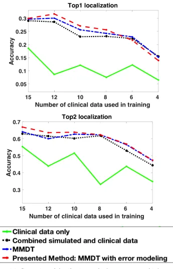
3.5 Comparison of classification results (top-one, top-two hits) among
alternative models on subject 1. Top1 indicate exact segment localization while Top2 combines the exact and neighboring
seg-ment prediction. . . 33
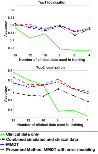
3.6 Comparison of classification results (top-one, top-two hits) among
alternative models on subject 2. Top1 indicate exact segment localization while Top2 combines the exact and neighboring
seg-ment prediction. . . 34
3.7 Comparison of classification results (top-one, top-two hits) among
alternative models on subject 3. Top1 indicate exact segment localization while Top2 combines the exact and neighboring
seg-ment prediction. . . 35
3.8 Comparison of regression results (mean and standard deviation)
among alternative models on each subject. . . 37
3.9 Results of retrospective emulation of the presented scheme of
progressive prediction. This schematic shows the mean reduc-tion in predicreduc-tion error with each added clinical data point,
along with the number of cases (N) tested in each step. . . 38
3.10 Two examples emulating how the presented scheme of progres-sive prediction would guide pace-mapping. Orange dots mark the targets, and yellow dots mark the models predictions in the
3.11 Comparison of localization accuracy between the presented method and the ECGI method in [27] (Subject 1, 2 and 3 respectively). STD(A): standard deviation of localization accuracy associated with di↵erent ECG beats when the same training data are used
(i.e., the same trial), averaged across all 20 trials. STD(B):
standard deviation of localization accuracy associated with the use of di↵erent training data (all 20 trials) for each beat,
aver-aged across all ECG beats from the same pacing site. . . 43
3.12 Schematic of pre-defined 14 segments model. . . 44
3.13 Comparison of classification accuracy when 14 versus 26
seg-ments are used for localizing the activation origin. . . 45
3.14 The e↵ect of keeping or removing extremity leads from the cal-culation of similarity scores on exact segment prediction for
subject 1 and subject 2. . . 48
3.15 Example of the combined regression and classification localiza-tion. The ground truth segment (A) and the predicted segment using the classification model (B). The predicted coordinate using the regression model is located on the far side of ground truth. Here, the clinician could decide the next pacing site to
be toward the predicted segment . . . 49
3.16 Confusion matrix results for subject1 of the 20 trails using 15 clinical pacing site within training. The upper box is a heatmap of the confusion matrix where the bar represents the average number of correct prediction for the specified segment while the lower box is a summary of which segments were easier to
predict which segments are harder to predict. . . 52
3.17 Confusion matrix results for subject2 of the 20 trails using 15 clinical pacing site within training. The upper box is a heatmap of the confusion matrix where the bar represents the average number of correct prediction for the specified segment while the lower box is a summary of which segments were easier to
3.18 Confusion matrix results for subject3 of the 20 trails using 15 clinical pacing site within training. The upper box is a heatmap of the confusion matrix where the bar represents the average number of correct prediction for the specified segment while the lower box is a summary of which segments were easier to
predict which segments are harder to predict. . . 54
3.19 Improvement in accuracy achieved by the presented domain adaptation methods when simulation data from Subject 2 or
Subject 3 are adapted to clinical data from Subject 1. . . 56
4.1 Overview of the presented method that includes two key
ele-ments. First, simulated ECG data from multiple patients are generalized through a MMD-VAE to remove patient-specific anatomical variations. Second, the generalized simulation data are adapted to clinical ECG data of a new patient through the
MMDT domain adaptation method. . . 62
4.2 An overview of the proposed domain generalization model
(MMD-VAE) which consists of three main components. At the heart of the model is VAE that encode then decode input features that extracted prior training the model. It also includes a classifi-cation layer that branch out from the latent space of the VAE. To align distribution from di↵erent source domains, MMD with RBF kernel is utilized at the latent space to ensure both decod-ing and classification encounter such a distribution alignment
which force invariant features to be employed. . . 77
4.3 Comparison of the proposed model, adapting directly
with-out generalization and patient-specific prediction model that utilizes patient-specific simulation data presented in chapter 3 when testing on clinical data from subject1. Top1 indicate ex-act segment localization while Top2 combines the exex-act and
4.4 Comparison of the proposed model, adapting directly with-out generalization and patient-specific prediction model that utilizes patient-specific simulation data proposed in chapter 3 when testing on clinical data from subject2. Top1 indicate ex-act segment localization while Top2 combines the exex-act and
neighboring segment prediction. . . 79
4.5 Comparison of the proposed model, adapting directly without
generalization and patient-specific prediction model that uti-lizes patient-specific simulation data proposed in 3 when test-ing on clinical data from subject3. Top1 indicate exact segment localization while Top2 combines the exact and neighboring
seg-ment prediction. . . 80
4.6 Examples of predicting pre-defined segments using three
di↵er-ent prediction models across three subjects. Label A indicates the ground truth segment which contains the origin of activation while B represents the predicted segment using patient-specific prediction model. Label C and D point out the predictions of a non-patient-specific model where simulated data from other subjects are used. The main di↵erence C and D is the
utiliza-tion of the proposed generalizautiliza-tion component. . . 81
4.7 t-SNE visualization of latent vectors when the training set
con-sist of subject2 and subject3 simulated data. Standard VAE with classification loss shows a separate hidden space between the two subjects. However, utilizing MMD to align the dis-tribution of the two subjects presents increased joined hidden
space. . . 81
4.8 t-SNE visualization of latent vectors when the training set
sist of subject2 and subject3 simulated data. It is hard to con-clude whether class labels appears more separable when align-ing the distribution via MMD. However, our results in table 4.2 shows an improvement of the accuracy which results obtained
3.1 Comparison of localization accuracy between the presented method
and the ECGI method in [27] (Subject 1). . . 58
3.2 Comparison of localization accuracy between the presented method
and the ECGI method in [27] (Subject 2). . . 59
3.3 Comparison of localization accuracy between the presented method
and the ECGI method in [27] (Subject 3). . . 60
4.1 The cross-recognition accuracy % of di↵erent domain
general-ization methods along with the proposed method MMD-VAE
on VLCS data set . . . 69
4.2 ground truth accuracy % L-SVM of patient-specific simulated
data . . . 71
4.3 The cross-recognition accuracy % of di↵erent domain
general-ization methods along with the proposed method on simulated
ECG using 26 segments . . . 71
4.4 The cross-recognition accuracy % of di↵erent domain
general-ization methods along with the proposed method on simulated
ECG using 14 segments . . . 71
1.1
Problem Definition
Machine learning and deep learning have seen significant breakthroughs that is promoting the overall outcome of sectors such as security, finance, natural language processing, and health-care [95]. However, one primary necessity for a successful machine learning solution is a large set of labeled data. In many fields, such labeled data are either costly, difficult, or impossible to acquire. For example, in some clinical tasks, the collection of labeled data may require expensive modalities, invasive procedures, or is physically not possible on the human subjects. To benefit from the advances of machine learning in those disciplines, there is a pressing need to explore and transfer knowledge from alternative sources of labeled data.
Computer simulation attempts to reproduce the behavior of a particular system via mechanistic models. Owing to the advances in mathematical mod-eling, numerical methods, and high performance computing, we can now sim-ulate more and more complex systems that closely replicate real-life chemical, biological or physical processes [8]. These simulation data provide a potential solution to the problem of the scarcity in real data. To leverage the data generated from computer simulation to facilitate learning from limited clinical data, however, involves two primary challenges.
First, simulating complex processes involves assumptions, simplifications, and potential errors inside the simulation model. As a result, the data
gener-ated inherently inhabit what we call adiscrepancy from real data. To be able
to leverage the abundance of simulation data, therefore, we first need to ad-dress and potentially learn this discrepancy when transferring the knowledge to real data to improve the performance of the predictive model.
Second, the generation of simulation data is generally tied to specific set-tings of model parameters. Many of these parameters have a considerable range of variations yet not necessarily relevant to the machine learning tasks of interest. To be able to transfer simulation data based learning to real data tasks , the knowledge extracted from simulation data must be generalizable across the parameters of variations that are irrelevant to the task of interest.
1.2
Research Objectives and Contribution
In this dissertation, we investigate the feasibility of leveraging simulation data to overcome the shortage of labeled real data, addressing the two key chal-lenges outlined above. We do so in a clinical task of localizing the origin of ventricular activation from 12 lead electrocardiogram (ECG): this task is rou-tinely carried out in treatment of cardiac arrhythmia, where the origin of the arrhythmia needs to be localized in the heart before it can be destroyed by in-tervention.Currently, this is either roughly done by clinician expertise, or more
precisely done by atrial-and-error procedure where di↵erent sites in the heart
are electrically stimulated, until locating the site where external stimulation reproduces the ECG morphology of the arrhythmia beats. A machine learn-ing model to directly predict the orgin of arrhythmia from its ECG data can improve the efficiency and accuracy of current practice. However, obtaining a real ECG data set with labeled sites of activation origin in the heart requires invasive procedures with artificial stimulation at multiple locations within the heart of a patient. In comparison, simulated ECG data can be generated at a much higher abundance with a much lower cost by virtually stimulating all possible locations in a computer heart model.
key challenges via the following contributions:
• By adopting the concept of domain adaptation, we address the
discrep-ancy between simulated and clinical data by learning the shift between the two domains using a large amount of simulation data and a small amount of clinical data. To account for potential local errors in a tion model, we devise a novel strategy to quantify the quality of simula-tion data utilizing a small number of clinical data. We then incorporate this quality measure into the process of domain adaptation between sim-ulation and clinical data. This adaptation happens in a patient-specific setting, in which we consider both classifying the origin of ventricular activation into one of 26 predefined ventricular segments, and regressing
the (x, y, z) coordinate of the origin of ventricular activation. Utilizing
previously developed simulation models [94], we modify existing domain adaption algorithms [43, 78] to address descripancy and internal error. This portion of the dissertation were published at the International Sym-posium on Biomedical Imaging ISBI 2018 [2] and IEEE Transaction in bioMedical Imaging TMI [1].
• By adopting the concept of domain generalization, we then address
the reliance of simulation data on patient-specific geometrical models
by learning to generalize simulated ECG data across subjects, before
transferring them to clinical data. We first present a novel domain-generalizing variational auto-encoder that, treating each subject as a domain, learns to remove domain-specific variations from ECG data.
The generalized simulation data from multiple subjects is then
trans-ferred to a small set of clinical data from a new subject via domain adaptation. This not only improves the generalizability of the knowl-edge extracted from the simulation data, but also removes the reliance on patient-specific image-based simulation for each new patient, reduc-ing the overall cost and increasreduc-ing the clinical applicability of leveragreduc-ing simulation data in clinical settings.
1.3
Dissertation Organization
Work
In this chapter, we will be introducing background information to incorporate the overall idea of this research. We start by a general introduction to machine learning to include some basic concept for a reader with no prior machine learning knowledge in Section 2.1.1. Next, we provide a literature review to the main machine learning topic used in this dissertation such as domain adaptation in Section 2.1.2 and domain generalization 2.1.3. To understand the clinical problem, Section 2.2 is a brief introduction where we first explain the Electrophysiological process and cardiac electrography in Section 2.2.1 and then explain the di↵erent types of cardiac arrhythmia in Section 2.2.2. The last subsection of this background will explore the current clinical practice to localize the origin of ventricular activation 2.3.
2.1
Machine Learning in Complex Scenarios
2.1.1 Introduction
Machine learning (ML) has revolutionized the decision-making process in var-ious enterprises when a computer program is involved. The formal definition of ML is the study of the algorithms and statistical models that computer systems use to achieve a particular task without using clear directions effi-ciently. It recognized as a subtopic of a more comprehensive science known
as Artificial intelligence. Based on the type of data used to train a particular model, there are three major types of ML (Supervised learning, unsupervised learning, and semi-supervised learning). When both input and the desired output data is available to train an ML algorithm, supervised learning is a logical choice. However, when the desired output is not available during train-ing, unsupervised learning is used to learn a particular pattern from the data. On the other hand, when some of the training set misses the desired output semi-supervised learning is utilized for that case.
Recent advances in machine learning algorithms have achieved significant success in many Artificial Intelligence tasks. However, such progress is based on the availability of large volumes of data. Unfortunately, large amounts of heterogeneous data that used for inference tend not to follow one distribution for a specific task. This can be defined as a discrepancy, domain shift or drift in the data distribution and caused by many di↵erent reasons. In machine learning, the general topic that focuses on designing a resolution for such a drift is known as domain adaptation which is a sub-field of a more broad topic known as transfer learning. The main idea of domain adaptation is to reduce the domain distribution mismatch when the training and testing samples come from di↵erent domains under one primary assumption which is the availability of labeled or unlabeled test (target) data.
A typical example of such a problem in computer vision is when changing lighting conditions, acquisition devices, or by considering the presence or ab-sence of backgrounds. A more specific example is when a large set of training data obtained via with digital single-lens reflex camera DSLR camera with good lighting is available. However, the main task is to classify of specific objects in images captured from a phone camera with poor lighting condition with the availability of a small labeled data from the same images. Similarly in speech recognition is when learning from one speaker and deploying an application targeted broad public speakers hindered by a di↵erence in back-ground noise, gender or tone. A comparable example can be found in many application that requires learning from data.
not available during the training process. A typical example of such a prob-lem in computer vision can also be in object recognition probprob-lem where the training data are standard image data sets while the test images are yet to be produced before specific training. Here, the main goal is to learn a robust and universal classifier that can generalize well to an unseen domain. In section 2.1.2 and 2.1.3, we introduce a literature review on these two topics since we utilize them to be the answer of the problem defined in section 1.1.
2.1.2 Domain Adaptation
Define a source domain where training data come from asDS and target
do-main where all test data comes from asDT. Transfer learning is a general field
of study that concern on transferring the knowledge from specific a classifier
that performs well in source domainDS to another classifier that doesn’t
per-form well in target domainDT. There are many di↵erent branches of transfer
learning such as multi-task learning, self-taught learning, and sample selection bias. A particular sub-field of transfer learning known as domain adaptation tries to mitigate the degradation of the performance of one classifier for data that are related but have a di↵erent distribution. Besides, this field of study
deals with the case of limited or no labeled data inDT. Our problem proposed
defined in Section 1.1 fits the exact requirements and assumption of domain adaptation.
Domain adaptation is a fundamental problem in machine learning and has gained a lot of attention recently in computer vision, natural language process-ing, and pattern recognition [67]. Many approaches were introduced as a way of solving this problem. The earliest and simplest approach known as feature augmentation methodology [20]. The main goal of that approach is to make a domain-specific copy of the original features of each domain. Each feature of the original domain is mapped onto an augmented space of dimensions. The rationale behind this approach is that both the source and target domain are transformed using these augmented features and then passed to underly-ing supervised learnunderly-ing. This approach was extended to learn heterogeneous data [53] and consider a manifold of intermediate domains [38, 39].
Figure 2.1: A conceptional illustration of an asymmetric domain transform [48] and a symmetric one [78], [48]
Figure 2.2: (A): An example of a linear classifier (shown as a decision bound-ary) trained on labeled source data with four classes. (B): labeled and un-labeled target data introduced to the model which creates a fitting problem to the target domains. (C): Existing SVM-based methods only adapt the features of classes with labels (crosses and triangles). (D): MMDT algorithm adjusts all points including unlabeled data from the target domain by utilizing a learned linear transformation. [43].
was proposed [19] that perform feature level alignment of the representations in the source and target domains.
Multiple algorithms investigated the possibility of modifying classifier pa-rameters (mostly SVM) to improve the classification performance for domain adaptation. Yang et al. proposed adaptive SVM [97] where source classi-fier training on source data and then adapted to a new classiclassi-fier for target data. Another algorithm that learns a target decision function and reduces the mismatch in the domain distribution using maximum mean discrepancy was proposed [7]. Besides, other algorithms focused on improving SVM for domain adaptation via selecting the best kernel. Adaptive multiple kernel learning is one of these algorithms where it learns a kernel function based on various base kernels [25]. A novel algorithm was introduced that jointly learn the matrix of feature transformation, and the parameter of an SVM classifier known as max-margin domain transform (MMDT) method was pre-sented to [43]. The key behind their approach is ”to simultaneously learn both the projection of the target features into the source domain and the classifier parameters themselves, using the same classification loss to jointly optimize both [43]” see Figure 2.2.
problems such as dictionary-based solution, land-mark notion, and deep learn-ing algorithms. For example, the dictionary-based approach is based on an idea that a high dimensional image or features can be coded in a few represen-tative atoms. Dictionary-based solution pioneered by [63] and then extended to handle domain shift problem in [60, 72, 82]. The landmark notion which is a subset of labeled data instances in the source domain that is mostly similar to target domain also used in domain adaptation [36, 37]. When a large train-ing set is available, a deep neural network is known to achieve state of the art performance in most of the problem. Several hierarchical deep learning model were introduced in domain adaptation [14, 35, 88]. Cheng et al. [14] in-troduced marginalized autoencoder for domain adaptation while Tzeng et al. introduced convolution neural network CNN architecture to exploit unlabeled and sparsely labeled target domain data.
Although there are a variety of approaches out there to solve the domain shift problem, selecting an appropriate method might seem complicated for any new challenge. In this research, we carefully weigh the assumption behind every algorithm and the type of approach. For example, dictionary-based were avoided because such an approach doesn’t use the valuable information in the source data. Also, deep neural networks type of works were also avoided because patient-specific data is considered very limited whereas deep network solution requires a large set of data. However, we looked at the approach type and how that is related to our data type and the weakness of every type so we can build on it to reach the best solution possible.
2.1.3 Domain Generalization
set of exemplar classifiers using one positive training sample and all negative training sample with a specific assumption such that positive samples should have a similar likelihood. More recently, Niu et al. [62] extended multiple in-stances of learning by creating one classifier per class per latent domain and integrated them to learn a more robust model.
Uncovering the domain-invariant features is the more common solution in the literature. Muandet et al. [58] minimizes the divergence across dif-ferent domains to obtain a domain invariant projection using a kernel-based optimization. Fang et al. [29] introduced Unbiased Metric Learning (UML) algorithm to learn a less biased distance metric among source domains then evaluated the proposed model on weakly labeled web images. More recently, an auto-encoding structure was employed to uncover invariant features. Ghi-fary et al. [32] introduced a multi-task auto-encoder for domain generalization by encoding with a common layer and decoding with domain-specific layers to reveal the invariant features among the domains. Recently Li et al. [52], employed a generative adversarial autoencoder and extracted the invariant features by alighting sources distribution and match with arbitrary prior at the latent space within the autoencoding structure to learn a generalized la-tent space among all domains. Their proposed model achieved state of the art result on the standard benchmark in computer vision data set on shallow structures.
2.2
Cardiac Electrophysiology and
Electrocardiog-raphy
2.2.1 Electrophysiology Process and Electrocardiography
Located in the ribcage between the right and left lungs, the human heart is a small cone-shaped muscular pump responsible for supplying the metabolic needs of the body by pumping blood to and from all necessary tissues. Anatom-ically speaking, the heart is divided into two main halves (right and left) separated by a septum muscle 2.3. Each half is divided into two chambers atrium and ventricle. A coordinated contraction of these chambers results in a successful pump of the blood throughout the body. These contractions are stimulated by electrical activity which starts from the sinoatrial (SA) node. This node, which is located in the right atrium, generates an electrical impulse that spreads to the atrioventricular (AV) node, located between the atria and the ventricles. After a small delay at the AV node, the electrical impulse prop-agates to the bundle of His, the bundle branches and Purkinje fibers, causing contraction of the ventricles. This normal rhythm repeats 60-100 times per minute in a resting state for most humans.
[image:28.612.128.526.463.628.2]The most popular non-invasive cardiac electrophysiology (EP) imaging
method is the standard 12-lead electrocardiography (ECG) which was pio-neered by Einthoven [26]. This conventional method is used to acquire body-surface potential dynamics to understand the cardiac conduction system. The reason this method is so popular because it is a non-invasive technique that translates the electrical impulse generated by the polarization and depolariza-tion of cardiac tissue into a wave-form. The standard 12-lead ECG uses six precordial leads on the anterior thorax and three leads placed on the right and left arm and left leg (to represent ground) 2.4.
[image:29.612.208.411.464.627.2]The ECG signal consists of 6 main segments as shown in Fig. 2.5. First, P wave which corresponds to the atrial depolarization while PR segment which represents the activation propagation through the AV node and Purkinje fibers. The most important segment is the QRS complex because it represents the depolarization of ventricular myocardium. This followed by ST-segment when action potential of all ventricular myocytes remains in the plateau and all the regions of the ventricles are in a depolarized state. Finally, T wave represents the last stage of cardiac contraction which is the repolarization of the ventricles. Since ECG represent a global summation of the electrical activ-ity within the heart, accurate inference of single action potential is a complex data interpretation problem. Thus, many research was dedicated to solving such an issue that was reviewed in Section 2.3.
2.2.2 Cardiac Arrhythmia
Any disruption to the regular pattern will eventually a↵ect the ability of the heart to e↵ectively contract and pump blood to the rest of the body. This disruption is generally known as arrhythmia, and there are many types re-lated to such a condition. Cardiac Arrhythmia can be defined as a group of conditions where the normal electrical activation cycle is interrupted. This revealed clinically in two distinct ways: tachycardia or fibrillation. Tachy-cardia is commonly known as a fast and uncontrolled heart rhythm in which the heart is shivers instead of contracting which a↵ect its ability to elevate blood to the rest of the body. Fibrillation can be defined as chaotic electric conduction of the heart which causes the heart to fibrillates [57]. Because of the di↵erent initiation mechanism between these two types, the main focus of this research will be on tachycardia. Tachycardia could originate anywhere in the heart. Some of these origins are generally known such as Wolf Parkinson White Syndrome (WPW) which a condition that might lead to tachycardia figure 2.6. In WPW, there is an extra pathway between the atria and the ventricles which can be obliterated directly.
[image:30.612.192.430.475.619.2]Unfortunately, some types of tachycardia have an unknown origin which makes them harder to treat. For example, scar-related ventricular tachycardia (VT), which is a significant cause of sudden death [85], involves electrical short
circuit formed by delicate strands of surviving tissue inside the myocardial scar as shown in figure 2.7. The treatment for such a problem is
interven-tional procedure known as ablation procedure that aims to cut o↵ the short
[image:31.612.175.447.513.596.2]circuit. Premature ventricular contraction (PVC) is another arrhythmia that causes tachycardia or fibrillation due to an extra heartbeat initiated mostly by Purkinje fibers in the ventricles. Generally, PVC is a benign abnormality in the heart and doesn’t require an invasive procedure. However, a frequent PVC does require similar ablation procedure to ablate the exact site within the ventricular.
Figure 2.6: Wol↵Parkinson White Syndrome abnormal activation [55]
2.3
Localizing Ventricular Activation
Localizing the origin of abnormal ventricular activation is of therapeutical im-portance in the treatment of many ventricular arrhythmias, such as premature ventricular contraction (PVC) and scar-related ventricular tachycardia [66,86]. Because the origin of ventricular activation largely determines the QRS mor-phology of 12-lead ECG [66], one current technique involves physically stim-ulating multiple myocardial sites until finding the site at which pacing
repro-duces the QRS morphology of the arrhythmia (i.e., the pace-matched site).
This practice – known as pace-mapping – is of a trial-and-error nature and
relies on a clinicians ability to interpret ECG data rapidly. Two main funda-mentally di↵erent computational techniques were used to solve this problem noninvasively. The first one is a data-driven approach that relies on machine learning to predict the origin of activation while the second one is a physics-based approach known as electrocardiographic imaging (ECGI). In this sec-tion, a review of both techniques will be presented with how both di↵er from each other.
2.3.1 Physic-Based Approaches
The Electrocardiographic inverse problem can be defined as the computation of epicardial potentials from body surface potentials. The most common ap-proach to solving such a problem is known as Electrocardiographic imaging (ECGI). ECGI can be defined as a functional imaging modality designed to noninvasively reconstruct epicardial potentials, electrograms, and isochrones from electrocardiographic body surface potentials. The inverse problem is known as to be ill-posed in the sense that small disruption in the data such as measurement noise or geometrical errors can cause large unbounded errors in the solution. Variety of ECGI methods comes from using di↵erent regular-ization methods to overcome this property. The most common regularregular-ization method is Tikhonov which imposes constraints on the magnitudes or deriva-tives of the computed epicardial potentials.
for the localization of the origin of ventricular activation in human. The application contexts are varied from localizing pacing sites [27, 80], PVC [49, 89] and scar-related VT [80, 92]. In [27], an ECGI method based on spline parameterization and transmural regularization was applied to localize the origin of ventricular activation on the same data set used in this research.
2.3.2 Data-Driven Approaches
A distinctive approach to ECGI is to utilize ECG data available from pa-tients and is known as a data-driven prediction model. SippensGroenewegen et.al [83] demonstrated that the QRS pattern of ECG allows discrimination among 38 di↵erent LV and RV segments of ectopic activations. The main idea of this approach is to apply machine learning approaches described in Section 2.1.1. This can be achieved by training a supervised prediction model on available ECG data with the known origin of activation as labels. The most popular types of data-driven approaches is a population-based solution in which machine learning is trained on ECG data collected from a large co-hort of patients. For example, Yokokawa et al. [99] pioneered this idea where a support vector machine (SVM) was used to localize the origin of activa-tion into ten predefined segments of the left ventricle (LV). Sapp et al. [79] followed a di↵erent strategy where they predicted the 3D coordinate of the origin of ventricular activation from 12-lead ECG. Deep learning models were recently proposed to account for inter-subject variations when learning to pre-dict the origin of ventricular activation from ECG data [15] [71]. However, these methods rely heavily on the population data, and the large anatomical and physiological variations in ECG data across individuals remain a challenge which leads to a limited accuracy.
and Clinical Domains
3.1
Introduction
Relying on pace-mapping data only to build a customized prediction model for each patient is a fundamental problem because it needs a sufficient number of locations to be paced. The abundance of simulation data, however, potentially provides knowledge about ECG originating from all possible locations on a ventricle, without requiring any pace-mapping to be carried out on a patient to train a model. Such significant advantage has motivated [45,69] to create a simulation based prediction model to localize the origin of ventricle activation as reviewed in Section 2.3.2. However, the accuracy of this type of model can be a↵ected by the discrepancy between the simulated and real ECG data due to assumptions, simplifications, and potential errors in the simulation model. In this chapter, we associate the above challenge with a common machine-learning scenario where there is limited data for training in the domain of in-terest (target domain) but an abundance of data in a related domain (source domain) [67]. Domain adaptation reviewed in Section 2.1.2 is a sub-field of transfer learning that addresses this challenge by considering the data distri-butional shifts between the source and target domain. Significant progress has been made in domain adaptation, especially in the field of computer vi-sion [67]. For example, in [78], a feature transformation matrix between the source and target domains was learned using metric learning. Subsequently,
a max-margin domain transform (MMDT) method was presented to jointly learn the matrix of feature transformation and the parameter of an SVM classi-fier [43]. Among existing works in domain adaptation, however, little attention is given to potential errors that may be non-uniformly distributed within the source data. We argue that, in the application context of this study, there is a potential presence of errors that vary across the simulation data, which needs to be quantified and incorporated into domain adaptation.
Specifically, using domain adaptation, we transfer the knowledge from sim-ulated ECG data to minimize the need for pace-mapping data in predicting the origin of ventricular activation. To account for potential errors in simulation data, we have devised a novel strategy to measure the quality of simulation data utilizing a small amount of clinical data. In a classification setting, we incorporate simulation errors into the SVM-based MMDT algorithm [43] and use it to localize the origin of ventricular activation into one of 24 predefined ventricular segments. In a regression setting, we incorporate simulation er-rors into the metric learning algorithm presented in [78] and use it to predict the 3D coordinate of the origin of ventricular activation. This allows us to introduce a scheme to improve the model with each added clinical ECG data, guiding the clinician progressively closer to the target site in real time.
We evaluate the presented method on three PVC patients in localizing a total of 75 pacing sites from 12-lead ECG [5]. Then, we compare the results with three alternative approaches to patient-specific modeling: a model trained only on clinical ECG data, a model trained on combined simulation and clin-ical data without considering domain shift, and a model trained on combined simulation and clinical data with domain adaptation but without addressing potential simulation errors. In this comparison, we investigate the e↵ect of using a varying number of clinical ECG data (4-15) for training. Further, we retrospectively emulate the proposed scheme of progressive prediction on the three patients. Finally, we compare the localization accuracy of the presented method with that obtained by a physics-based approach, known as electro-cardiographic imaging (ECGI), on the same patients [27]. Our results show that the presented method has the potential to provide real-time guidance for localizing the origin of ventricular activation within a small number of pacing sites. We make the following key contributions in this chapter:
• We introduce the concept of domain adaptation to transfer knowledge
order to localize the origin of ventricular activation from 12-lead ECG data.
• We devise a novel method to quantify and incorporate non-uniformly
distributed simulation errors to improve the accuracy of domain adap-tation.
• We introduce and emulate a strategy to progressively guide clinicians to
the origin of ventricular activation in real time. This emulation study were adopted from [87]
• We demonstrate the efficacy of incorporating knowledge from simulation
data while addressing the discrepancy between simulated and clinical data through a comprehensive comparison study.
• We compare the performance of the presented data-driven approach to a
physics-based approach in localizing the origin of ventricular activation on the same dataset, with an in-depth discussion of the di↵erences in performance
3.2
Image-based ECG Simulation with Error
Quan-tification
The presented method consists of two main elements. First, using a patient-specific model, a large set of ECG data is simulated from ventricular activation originating at various locations of the ventricles. Second, using a small amount of clinical data, the quality of the simulated ECG data is measured according to its origin of ventricular activation.
3.2.1 Image-based Patient-specific ECG Simulation
Image-based Personalized Anatomical Models
From cardiac tomographic scans (e.g., CT or MRI) of a patient, a 3D
bi-ventricular model is first customized to the patient. a 3D fiber structure of the patient-specific ventricular model is constructed to allow anisotropic conduction. Fiber orientations at the epicardial and endocardial surfaces are mapped from a canine ventricular fibrous model established in [59]. Fiber orientations inside the myocardium are then interpolated from those on the surface, assuming a linear counterclockwise rotation [61].
Because ECG data are a↵ected by the anatomical shape of the torso and the position of surface electrodes [11], a patient-specific torso model is also extracted from the tomographic scans of a patient (subject). We assume the torso to be an isotropic and homogeneous volume conductor.
Personalized Cardiac Electrophysiological Modeling
On the patient-specific ventricular model, activation sequences originating at di↵erent ventricular locations are simulated using the macroscopic
mono-domainAliev-Panfilov model [4]:
@u
@t =r(Dru) cu(u a)(u 1) uz
@z
@t =✏(u, z)( z cu(u a 1))
(3.1)
where u stands for the transmembrane potential (TMP), z for the recovery
current, andDfor the di↵usion tensor. ✏,c, andaare parameters that control
local TMP shape. This model is solved numerically on the patient-specific ventricular model using the mesh-free method as detailed in [94]. A large set of simulation data is generated using each node in the ventricular mesh as the origin of ventricular activation. On average, we consider a ventricular mesh
with a spatial resolution of⇠5-mm. This is the size of a typical ablation lesion
Simulation of Patient-specific ECG Database
On the patient-specific heart-torso model, the relationship between the TMP
and the surface ECG is governed by thequasi-static electromagnetic theory:
kr2 tk(r) =r( Di(r)ru(r)), 8r2⌦h (3.2)
tr2 t(r) = 0, 8r2⌦t/h (3.3)
whereDiis the intracellular conductivity tensor, kis the bulk conductivity, t
is the torso conductivity, tk is the extracellular potential in the myocardium,
tis the body surface potential,⌦h is the domain of the ventricular mesh, and
⌦t/h is the domain between the ventricular surfaces and body surface. These
equations are solved on the 3D patient-specific heart-torso model using the combined Boundary-Element and Meshfree strategy as described in [94].
Twelve-lead ECG can be extracted from the simulated body-surface ECG maps, producing a simulated database of 12-lead ECG with known origin
of ventricular activation. Because the Aliev-Panfilov model is unitless, the
simulated ECGs are scaled in both amplitude and time to a physiologically
meaningful range. The amplitude is scaled by 110 90 to bring the
Aliev-Panfilov model output (0 1) to the physiological range of TMP ( 90 20
mV). For temporal scaling, a mean ratio is calculated between QRS durations in simulated and clinical ECG data, which is then applied to all simulated ECGs.
3.2.2 Quantification of ECG Simulation Quality
A general discrepancy exists between simulated and clinical data due to as-sumptions and simplifications involved in simulation models. This discrepancy, however, may vary spatially. As a result, simulated ECG data originating from certain ventricular locations may be less similar to clinical ECG data than to data originating from other ventricular locations. In our dataset, simulated ECG data originating within the septum are in general observed to be less sim-ilar to their clinical counterparts, compared with ECG data originating from other ventricular locations. Therefore, we propose to model this spatially non-uniform quality of simulation by utilizing a small amount of available clinical ECG data obtained during pace-mapping.
We denote the simulated data (source domainDS) as {xsi}Ni=1 with labels
where the number of simulated dataN is significantly larger than the number
of clinical data M. We measure the quality of the simulated ECG data as a
function of the origin of the ventricular activation in the following three steps:
1. Measure the quality of simulated ECG data using available clinical
data : Correlation coefficients between a paced ECG and the target ECG
from the ventricular tachycardia (VT) are a primary metric used to iden-tify the pace-matched site in conventional pace-mapping [22]. We therefore base the quantification of simulation quality on this metric. Given a pair
of simulated xsj and clinical ECG data xtj originating from the same
loca-tion, we measure their similarity using the Pearson correlation coefficient:
⇢j = |cov(xsj,xtj)/( (xsj) (xtj))|. This yields a partial map that shows how
the quality of the simulation data varies in space at limited locations where clinical ECG data are available.
2. Learn the spatially-varying similarity map across the ventricles: To es-timate the quality of the simulation data at locations where clinical ECGs are
not available, we train a regression model for the similarity measure⇢(x, y, z)
as a function of the spatial coordinate (x, y, z). We use support vector
regres-sion (SVR) model with the radial basis kernel [24]. Trained with⇢j at limited
spatial locations obtained in Step 1, it generates the similarity measure across the ventricles.
3. Scale the similarity map to emphasize the penalty for large errors: We intend to utilize the similarity map to recognize and penalize inaccurate simu-lation data in domain adaptation. We argue that simusimu-lation data of reasonable
quality (e.g.,⇢(x, y, z) 0.5) should be treated similarly, whereas a drastically
increasing penalty should be applied as the quality decreases below that range (e.g.,⇢(x, y, z) <0.5). We thus scale ⇢(x, y, z) with a modified sigmoid
func-tion: (x, y, z) = 1/(1 +e 10⇢(x,y,z) 0.3), which can be visualized in Fig. 3.1.
Evaluating (x, y, z) on each node in the cardiac mesh yields us the quality
measure{ s
i}Ni=1 for all simulated ECG data.
0 0.2 0.4 0.6 0.8 1
Estimated input score (
ρ
j
)
0 0.2 0.4 0.6 0.8
[image:41.612.165.460.127.364.2]Estimated output score (
Figure 3.1: Mapping function. This modified sigmoid function transforms
⇢i 0.5 to a similar output score i, but it transforms⇢i<0.5 to a drastically
decreasing output score i. Th red dotted line shows an example when the
input score is 0.5 the output estimated score will be 0.88
more clinical ECG data were incorporated for training.
3.3
Domain Adaptation with Uncertainty
Figure 3.2: Illustration of the change in the learned similarity map as the number of clinical data increases (middle panel), in comparison with examples
of clinicalversus simulated ECG data with their actual correlation coefficients
(CC) at selected sites (A, B, C, and D). This provides an example of the agreement between the actual simulation quality at selected sites and the learned similarity map as more clinical data are used for training.
3.3.1 Regression-based Domain Adaptation
Regression-based domain adaptation has not been well investigated, except in a theoretical study in [17]. Here, we present a distance-based approach to first learn an optimal distance metric between the simulated and clinical domain, and we then use the learned distance metric in combination with the k-nearest-neighbor (kNN) method to predict the coordinates of the activation origin of ventricular activation from ECG data.
To learn the distance metric between a source and target domain, Saenko et al [78] presented an approach based on the concept of Mahalanobis
dis-tance as described in [21]. Given data in the source domain xs
i and target
domain xt
j, their Mahalanobis distance can be measured by dW(xsi,xtj) =
q
(xs
i xtj)TW(xsi xtj), parameterized by a positive-definite matrixW. To
learn W from training data, dW(xsi,xtj) is regularized to be close to a given
and dissimilarity constraints [21]:
min
W KL(p(x;W0)||(p(x;W))
s.t. dW(xsi,xjt)u yis=yjt
dW(xsi,xtj) l yis6=yjs
(3.4)
where KL is the Kullback-Leibler divergence, andp(x;W) = Z1 exp ( 12dW(x, µ))
is a multivariate Gaussian, with Z being the normalizing constant and W 1
the covariance of the distribution. W0, per the standard definition of
Maha-lanobis distance, is often taken as the covariance matrix of the dataset which
consist both source and target domains. The distance between W0 and W
is minimized by minimizing the Kullback-Leibler divergence between the two multivariate Gaussian [78]. The constraints specify that two data points
shar-ing the same label should have a dW smaller than a relatively small value
of u; otherwise, their dW should be larger than a relatively large value of l.
In practice, for example, u can be assigned as the 5th percentile value of all
Euclidean distances between the source and target data, and l as the 95th
percentile value.
While the similarity/dissimilarity between two data points is in a binary fashion in the setting of classification, it is in a continuous fashion in the set-ting of regression. Here, we argue that the dissimilarity between the ECG data originating from two ventricular locations should be proportional to the distance between the two origins. Therefore, we modify the
dissimilar-ity lower bound of l to be a function of the distance between two origins:
l(dstij) = (B A)(dstij mindst)
(maxdst mindst) +dstij, where dstij is the Euclidean distance between
a source origin (coordinateyis) and a target origin (coordinateytj) of interest,
dst includes Euclidean distances between every pair of source and target data,
andB andA are pre-defined ranges of lower bound in terms of the percentile
values indst. Here, we use 80th and 95th percentiles. In this way, the closer
the pair is in the origin of activation, the smaller the lower bound will be for their dissimilarity measure.
For source and target ECG originating from the same location, the
simi-larity upper bound uholds with the exception that we also take into account
the simulation quality: if si betweenxsi andxtj is lower than a certain
optimization problem:
min
W KL(p(x;W0)||(p(x;W))
s.t. dW(xsi,xtj)u ysi =ytj, si ✏
dW(xsi,xtj) l(dstij) yis6=yjt
(3.5)
where✏= (N1005 + 0.5) (x, y, z) andN is the number of source data. This is
solved as described in [21].
Progressive Prediction for Real-time Guidance: The ultimate con-text in which we envision the application of the proposed regression model is to provide real-time, continuous guidance in the process of pace-mapping We thus present a scheme in which, at the beginning of the pace-mapping procedure, an initial prediction of the location of the origin of ventricular acti-vation will be obtained using only the simulation data. The clinician will pace the predicted location and examine the morphology of the generated clinical 12-lead ECG. The model will be updated by the newly obtained 12-lead ECG data using the domain adaptation regression technique described above. A new prediction will be made and new pace-mapping data will be collected at the predicted site. This process will continue until the clinician finds a pace-matched site of interest. As more pace-mapping data become available for adapting the model from the simulated data, the presented model is expected to guide the clinician progressively toward the target site.
3.3.2 Classification-based Domain Adaptation
The classification setting involves localizing the origin of ventricular activation into one of several predefined anatomical segments of the ventricles – a problem frequently considered in previous studies [100]. In this setting, we use a classic domain adaptation technique known as the MMDT [43]. It simultaneously
learns a linear transformation W between the source and target domain in
source and transformed target data, formulated for a K-class problem as:
min
W,✓k,bkJ(W,✓k, bk) =
1
2||W||
2 F + K X k=1 " 1
2||✓k||
2 2
+CS
ns
X
i=1
⇣ ysi,
xsi
1 ,
✓k
bk
!
+CT
nT
X
i=1
⇣ yit,W·
xti
1 , ✓k bk !# (3.6)
where the affine hyperplane ✓k and o↵set bk are parameters of the SVM, and
k= 1,2,· · ·, K. ⇣() is the hinge loss with the corresponding parameters CS
andCT. In the standard MMDT, a predefined value ofCS andCT is used for
hinge losses across all source and target data, respectively. Here, we propose that the parameter controlling hinge losses from the source domain vary with
each simulated ECG dataset. Specifically, we multiply CS by the quality
measure s
i that is associated with each individual xsi as defined in section
3.2.2. This gives us a modified cost function:
min
W,✓k,bk
J(W,✓k, bk) =
1
2||W||
2 F + K X k=1 " 1
2||✓k||
2 2
+CS
ns
X
i=1
s i.⇣ ysi,
xsi
1 ,
✓k
bk
!
+CT
nT
X
i=1
⇣ yti,W.
xti
1 , ✓k bk !# (3.7)
In this way, a high-quality simulation ECG signal with si ⇡ 1 will be
una↵ected during the optimization, whereas a low-quality ECG signal with
0< s
i <1 will have a reduced e↵ect on the optimization of SVM parameters,
until close to having no e↵ect as si approaches 0. Following [43], equation
(7) is solved by an iterative procedure. In each iteration, SVM parameters are first estimated using both source data and target data transformed by the
3.4
Experiments and Results
In this section, we first describe the simulated and clinical data used in the experiments, as well as the data processing procedure. Next, we compare the performance of the presented method with three alternative patient-specific prediction models in terms of both classification and regression settings. Then, we present results from retrospectively emulating the use of the presented regression method in guiding ablation procedures. Finally, we compare the presented method with an alternative physics-based approach on the same dataset.
3.4.1 Data and Data Processing
The presented method is evaluated on 12-lead ECG data collected during endocardial pacing from three PVC patients, made available through the Ex-perimental Data and Geometric Analysis Repository (EDGAR) database [5].
For each patient, there is a mean of 25±6 ECG data points from distinct sites
of endocardial pacing with known coordinates. From each pacing site, a mean
of 28±8 ECG beats are available.
Patient-specific heart-torso geometry models are also available for each patient, from which the simulated 12-lead ECG is generated as described in
section 3.2.1. On average, 1637±35 ECG data are simulated for each patient,
corresponding to origins of ventricular activation evenly distributed
through-out the 3D myocardium at a resolution of 4.9±0.8 mm.
QRS integrals are extracted from each beat of the clinical ECG data and simulated ECG data. To capture the morphology of the QRS complex, we define features in the form of incremental integrals at 10-ms intervals until reaching a maximum of 120-ms. This results in a 12-dimensional feature vector on each ECG lead and, across 12 leads, a 144-dimensional feature vector. Fig.3.3 provides two representative examples of histograms of the extracted
ECG features in simulated versus clinical data: Even though the amount of
clinical data is limited, the shift in data distribution between the two domains is visible, underscoring the need for domain adaptation techniques.
Figure 3.4: Schematics of the pre-defined 26-segment model.
of the origin of ventricular activation are used.
3.4.2 Classification Results
In the classification setting, the presented model (referred to as MMDT with error modeling) is compared with three alternative patient-specific modeling approaches: a standard SVM trained on clinical data only, a standard SVM trained on combined simulation and clinical data without considering domain adaptation, and an SVM trained with the standard MMDT method for domain adaptation but without considering simulation errors. All four models are trained and tested using the same software package [13]. For the standard SVMs in the first two models, the parameter C for hinge losses is tuned using 5-fold cross-validation. Parameter C from the second model, tuned on simulation
data, is then used asCT for the two MMDT-based models withCS set to be
0.05.
repeats 20 times for each specified training data set size to obtain a measure of mean accuracy with the associated variance.
For each given model, the percentage of time that the prediction of the
origin of ventricular activation is correct (i.e., that the origin is localized into
the correct segment) is reported as the top-one hit. We have observed that, when the prediction of the origin of ventricular activation is incorrect, the predicted segment tends to lie immediately adjacent to the actual (correct) segment. Thus, we also report the percentage of time that the origin of ven-tricular activation is localized into the correct segment or into the segment immediately adjacent to the correct segment (top-two hit). Figs. 3.5,3.6 and 3.7 shows the mean localization accuracy of each model for the three subjects. As shown, a model trained exclusively on clinical data has a reasonable accuracy when the number of training data is not too low (solid green line). However, this accuracy quickly drops as the number of clinical data decreases. By incorporating simulation data without considering the domain shift be-tween simulation and clinical data (black dotted line), the classification ac-curacy shows a general improvement. However, the amount of improvement varies from subject to subject, which might be related to varying levels of agreement between simulation and clinical data. Note that the amount of improvement is significant when the number of clinical data is small. With modeling approaches that include domain adaptation (blue dotted line) and domain adaptation that accounts for the non-uniform simulation errors (the presented method; red dotted line), we see further improvements in accuracy. The presented method, in general, achieves the highest accuracy except in occasional cases. The improvement margins that these two methods yield, however, again vary from case to case.
3.4.3 Regression Results
In the regression setting, similarly, the presented method is compared with the following three models: a standard KNN using clinical ECG data only, a standard KNN using simulation data only, and a KNN based on the optimal distance metric learned between simulated and clinical domain using equation
(5) but without removing data with low simulation quality ( s
i <✏) from the
similarity constraint. For all KNNs, no kernels are used and the number of
Figure 3.9: Results of retrospective emulation of the presented scheme of progressive prediction. This schematic shows the mean reduction in prediction error with each added clinical data point, along with the number of cases (N) tested in each step.
the training set.
The comparison study is carried out in a similar setting to that described in section IV-B, repeated as the number of clinical data used in training decreases and repeated for random splitting of training and test data in each case. The regression accuracy is reported in terms of the Euclidean distance between the predicted and actual origin of activation. Fig. 3.8 shows the mean prediction error as a function of the number of clinical data used in training for each of the three subjects.
Similar to the observation in the classification setting, when only clinical data are available for training (red bar), the mean prediction error increases substantially as the number of clinical data decreases. The incorporation of simulation data results in a moderate reduction in the prediction error when the number of clinical data is small (blue bar). However, when the number of training clinical data is not low, the prediction error is significantly higher. This demonstrates that the di↵erence between simulated and clinical data may have a more significant e↵ect on regression than on classification. Introducing domain adaptation results in a further reduction in prediction error in most of the cases (green bar), although the error is still higher or similar to that obtained by using clinical data only. This indicates that domain adaptation is able to address the shift between simulation and clinical data, but only to a limited extent.
simulated and clinical data in a regression setting.
Similar to the observation in the classification setting, the performance improvement of the presented method is not as good when the number of clinical data for training is low. This again may be attributed to the difficulty in obtaining a good estimate of the simulation error when the number of clinical data is limited.
3.4.4 Emulation of Clinical Procedures
Next, we utilize the available pace-mapping data on each patient to retro-spectively emulate how th
![Figure 2.1: A conceptional illustration of an asymmetric domain transform [48]and a symmetric one [78], [48]](https://thumb-us.123doks.com/thumbv2/123dok_us/24283.1885/24.612.182.442.144.386/figure-conceptional-illustration-asymmetric-domain-transform-and-symmetric.webp)
![Figure 2.3: An interior view of the frontal section of the human heart [64]](https://thumb-us.123doks.com/thumbv2/123dok_us/24283.1885/28.612.128.526.463.628/figure-interior-view-frontal-section-human-heart.webp)
![Figure 2.4: placement of the precordial leads in electrocardiography [41]](https://thumb-us.123doks.com/thumbv2/123dok_us/24283.1885/29.612.208.411.464.627/figure-placement-precordial-leads-electrocardiography.webp)
![Figure 2.5: Schematic diagram of normal sinus rhythm for a human heart asseen on ECG [6]](https://thumb-us.123doks.com/thumbv2/123dok_us/24283.1885/30.612.192.430.475.619/figure-schematic-diagram-normal-sinus-rhythm-human-asseen.webp)
![Figure 2.6: Wol↵ Parkinson White Syndrome abnormal activation [55]](https://thumb-us.123doks.com/thumbv2/123dok_us/24283.1885/31.612.175.447.513.596/figure-wol-parkinson-white-syndrome-abnormal-activation.webp)