Southern Region Engineering Conference 11-12 November 2010, Toowoomba, Australia SREC2010-F2-1
Analysis of Data to Develop
Models for Spray Combustion
Jason Clarke, Andrew P. Wandel
Computational Engineering and Science Research Centre Faculty of Engineering and Surveying
University of Southern Queensland Toowoomba, 4350, Australia
E. Mastorakos
Department of Mechanical Engineering Cambridge University
Cambridge, CB1 2PZ, UK
Abstract— Modern combustion systems are being designed to operate closer to the lean combustion limit in order to improve fuel economy, reduce operating noise and reduce the production of pollutants. However, this increases the chances of misfiring occurring, particularly when the fuel is injected into the combustion chamber in liquid form and heat is required to vaporise the fuel so that it is available for combustion. Modelling of this process is required to aid in the development of new combustion systems; the Conditional Moment Closure (CMC) model is well suited for such modelling. However, the behaviour of key terms in the CMC transport equation—the conditional scalar dissipation, mixture fraction probability density function (PDF) and conditional source term—is not understood well for this case. Note that the conditional source term only appears when one of the key reactants changes state to become a gas. A Direct Numerical Simulation (DNS) study was performed to collect data on successful and unsuccessful combustion when the fuel is fully comprised of liquid droplets in cold air and spark power is used to evaporate the fuel and ignite the mixture. The data from the DNS are being used to develop models for the three key terms required for CMC modelling.
Keywords-spray combustion; DNS; CMC;
I. INTRODUCTION
In the motor industry today, almost all petrol engines have adopted the use of injectors to supply fuel to the combustion chamber. The use of injectors has allowed a much greater ability to control the parameters of spark assisted spray ignition than carbureted engines. Some parameters which may be adjusted are: droplet size, droplet density, spray pattern, spark intensity and duration. The advent of fuel injection has also meant that the mixing of fuel and oxygen now takes place in the combustion chamber.
Increasingly, governments and social pressure have required engines to become more efficient. For the best chemical efficiency, fuel and air should be burnt at the stoichiometric mixture (the amount of fuel and air is such that both are consumed completely—there is no excess of either): for octane fuels, the air-to-fuel ratio (mair/mfuel) should be 14.7. However, traditionally, the mixture has been rich, or an air-to-fuel ratio in the range of 12.5–13.3, to reduce the chance of engine misfires. This, however, leads to unwanted pollutants, such as HC, CO and NOx.
Modelling spark-assisted spray ignition exactly using Direct Numerical Simulations (DNS) would assist in further understanding the parameters which lead to the cleanest burning of fuel and would allow the design of injection systems which develop those parameters. However, the current processing power of computers has not allowed the usage of DNS for gaseous combustion systems for volumes larger than the order of 1 cm3 [1], therefore Computational Fluid Dynamics (CFD) is required to model real applications. However, because little is known about the evaporation of droplets in combustion systems, models for CFD must be developed [2].
Modelling of gaseous phase combustion is simpler than droplet combustion because the fuel is already present in the correct phase. In spray combustion, however, the droplets must first be evaporated by an area of localised high temperature (which may be created by the spark energy or compression of the gas), and must continue to be evaporated by the flame front in order to continue releasing fuel to the system [3]. Literature published on the modelling of turbulent combustion of two phase systems has been restricted to the last couple of decades as the processing power required to perform numerical simulations has become available.
While there have been numerous studies into spray combustion using DNS [3, 4, 5, 6], no large-scale studies have been performed using the Conditional Moment Closure (CMC) model [2]. This is because there is limited understanding of the behaviour of the key coefficients in the CMC equation in the presence of evaporation. While some effort has been made using 2-D DNS in an autoignition configuration [7], this is of limited value because of the artificial nature of 2-D DNS.
The current study aims to reduce the gap in knowledge by analysing 3-D DNS to generate models for the key coefficients in the CMC transport equation so that large-scale modelling may be performed for sprays.
II. THEORY
dependent variables), are evaluated by substituting the average values for the variables. The errors are caused by ignoring the correlation between these variables, which are generally significant compared to the corresponding averages. The CMC model overcomes this difficulty by using conditional averages, whereby variables are averaged for a specified value of the mixture fraction. This effectively averages over a smaller region of space than a conventional CFD cell, therefore is more accurate and also often causes the correlations to become negligibly small. For homogenous, two phase systems, the form of CMC is:
2
2
Y Z Y Z
N Z W Z S Z
t Z
∂ ∂
= + +
∂ ∂ (1)
where:
• = mixture fraction, or proportion of the mixture that was originally fuel;
• = mass fraction of fuel (mass of fuel normalised by total mass);
• = conditional scalar dissipation (equivalent to viscosity);
• = conditional chemical source term (gain/loss due to chemical reactions);
• = conditional generation due to droplet evaporation.
It is expected that will vary significantly from its behaviour in a single-phase system, so requires further modelling, as will P(Z), the mixture fraction probability density function (PDF), which is required to obtain averages via:
( )
1
0
Y =
∫
Y Z P Z dZ . (2)The additional source term for spray combustion, , also requires modelling. The other term in the CMC equation, , may be modelled by using the conditional averages of mass fraction and temperature in the Arrhenius reaction formula.
Wandel et al. [3] performed a DNS study on a small, three-dimensional control volume in order to investigate the characteristics (droplet size and spacing) that would lead to full combustion of a fine mist of fuel. The control volume was cubic, with 128 nodes along each edge, with the following characteristics:
• Two directions (y and z) were periodic (droplets which flow out of the boundary re-enter through the opposite boundary);
• One direction (x) was “partially non-reflecting” (the gradient at the boundary is zero, droplets do not re-enter);
• Droplets were uniformly distributed throughout the y
and z directions, and between and in the x
direction, where L is the cube’s side length;
• The spark was centred in the control volume, and deposited energy for a predetermined period of time. The quantities required for the CMC model were calculated from this study and analysed for the current work.
III. DNSDATA AND CURVE FITS
When the flow initially consists of cold air with the fuel solely contained in droplets dispersed throughout the air, there are three main regimes (“zones”) that may be observed in a successful burn when a spark is turned on, then off:
• Initial stage (<7 µs): Little fuel vapour exists, combustion is almost non-existent, there is a rapid release of fuel to the system as the spark evaporates fuel.
• Intermediate stage (7–165 µs): The spark is either still on, or there is a strong residual effect from the spark and the droplet evaporation rate becomes steady-state. • Final stage (>165 µs): No residual effect from the
spark exists, droplet evaporation is steady-state for the remaining droplets (many are completely evaporated), flame propagation is strong.
For the purposes of fully characterising the data, another stage was introduced. This stage occurs before the initial stage, and for this very brief period, all quantities approximate the initial conditions before the spark begins evaporating fuel. This stage will be referred to as zone 0.
The initial droplet density was such that the equivalence ratio in the droplet region was two. When averaged over the entire computational domain, this was the stoichiometric ratio. The combustion took place over 2.80ms.
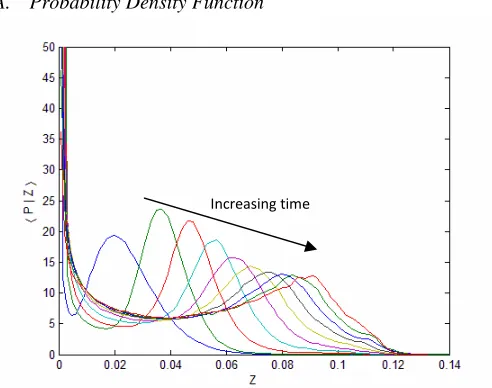
[image:2.595.310.556.433.627.2]A. Probability Density Function
Figure 1. The Probability Density Function over the length of the combustion.
Fig. 1 shows the PDF of the mixture fraction, P(Z), throughout the control volume. As the fuel evaporates, large regions develop that become rich, owing to the high equivalence ratio inherent in the initial distribution. The variation in mixture fractions is due to the presence of localised high mixture fractions (such as the zone around the droplet in which the mixture fraction is high due to evaporation of the droplets), and areas where fuel is sparse (such as the spacing between the droplets). However, the fuel rapidly diffuses away from the droplets, as indicated by the probability of locations
having an equivalence ratio of 2 being insignificant (the stoichiometric mixture fraction was ). Initially, the mixture fraction PDF shows that most fuel was still unavailable to the system as the droplets were yet to evaporate. However, as combustion progresses, more fuel is available to the system, which is shown by the progression of the secondary peak up to .
It is evident the functions are not self-similar and seem to be a function of time. In this state, P(Z) is difficult to characterise. The functions can be made self similar by considering the Favre PDF, defined as where is the conditional density and is the mean density. The mixture fraction was also normalised by the mean mixture fraction: . The approach of normalising the quantities by a mean quantity will be adopted throughout the analysis as average values are quite readily predicted at any point during the combustion and this should make any model generally applicable for any case.
Fig. 2 shows the Favre PDF for the four distinct zones of combustion. Zone 0 refers to combustion at very small values of time, before significant changes are made to the probability density function by the evaporation of fuel. Initially, the distribution takes the form of a β-function PDF, with the errors in the location of the δ-function near Z = 0 being due to the rapidly increasing mean mixture fraction. However, the error will be negligible as zone 0 represents a very small period in time in comparison to the length of the combustion.
The plot of the zone 1 PDF shows the effect of the spark evaporating droplets to release fuel to the system. A Gaussian peak can be seen to form at in addition to the β-function PDF, which still dominates the behaviour for . Further analysis reveals a secondary Gaussian peak at . The function to describe the behaviour for zone 1 is a composite function of the form:
(3) where An is a constant, is a β-function PDF and is a Gaussian PDF. The formula for a β-function PDF is:
(
)
(
)
( ) ( )
1 1
1
; , n n
n
Z a b Z
B Z
b a b a b a
α β
α β
α β
α β
− −
Γ + − −
=
− Γ Γ − − (4)
with α and β the shape parameters while is the range where . A Gaussian PDF is solely a function of the mean, µ, and standard deviation, σ :
( )
[
]
2
2 2
1 exp 2
n n
Z
G Z µ
σ πσ
−
= −
(5)
For zone 1, the coefficients of the Gaussian PDFs are:
while the shape parameters for the β-function PDF are:
The resulting fit is shown in Fig. 2. Some error is evident around the primary peak which may also be due to the normalisation of the abscissa, while the composite PDF does not predict the interface between the β-function PDF and secondary Gaussian PDF for . In addition, there is some transient development around the secondary peak which is not completely captured by the primary Gaussian PDF. The degree to which these errors will affect the recreation of the probability density function will be seen in further analysis.
while the shape parameters for the β-function PDF are:
In zone 2, the system becomes more stable and the secondary Gaussian function has more effect on the final function. The mean mixture fraction is relatively stable during this period, so the peak near Z = 0 is reasonably accurately predicted, while there are some errors for .
In zone 3, the system becomes stable and therefore the Favre averaged PDFs during this time are self-similar. Again, the composite function (3) is used to characterise the zone with:
while the shape parameters for the β-function PDF are:
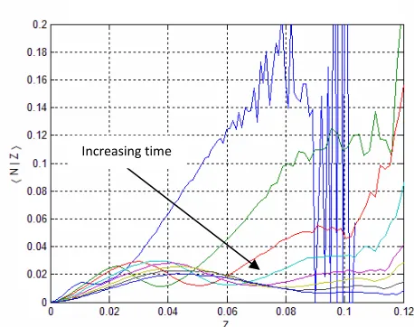
Figure 3. Conditional scalar dissipation versus mixture fraction for the length of the combustion.
B. Conditional Scalar Dissipation
A plot of conditional scalar dissipation over the length of the combustion is shown in Fig. 3. The scalar dissipation is defined as where is the diffusitivity and is the gradient of Z. The scalar dissipation is large for large values of Z because this corresponds to areas immediately adjacent to the droplet surfaces, which provide the source of Z. Throughout combustion, a peak progressively shifts from low values of Z to high values of Z, which indicates the development of the flame front, which eventually stabilises.
The large fluctuations in the data for large values of Z
(particularly Z > 0.09 for the first instant in Fig. 3) are due to statistical errors, corresponding to low values of probability. Because there were few nodes with large values of Z, the sample sizes were low for the conditional averages at these high values. Where no samples were available, the conditional average was set to zero. Therefore, as a general rule, values of
Z corresponding to will be neglected.
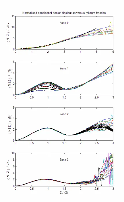
Again, the data is not self-similar and seems to be a function of time. This is rectified by normalising the conditional scalar dissipation by the mean scalar dissipation.
The plots of conditional scalar dissipation versus mixture fraction for each of the four zones of combustion are shown in Fig. 4. Zones 0, 2 and 3 are, for most values of Z, self-similar. The conditional scalar dissipation undergoes a transition in zone 1 where a peak and trough form progressively. While a single polynomial was used to model zone 0, three cubic splines were used for the remaining zones.
The fit for zone 0 is shown on Fig. 4. For clarity, large values of , which correspond to erroneous values of , are omitted. The value of corresponds to a probability of . This is a higher probability than the target previously set of , but has been deemed to be appropriate given that the data becomes erratic at values of larger than this.
The fit for zone 0 is a second-order polynomial which is forced to pass through the origin. The function is:
( )
20 3282 0 2706
n n n
f Z = . Z + . Z (4)
which is quite good for values of Z which have significant probability.
The curves for zone 1 are dependent on time and the first two cubic splines were constructed to pass through the maxima and minima with the gradient forced to be zero. The function for the position of the maxima with respect to time is:
2 max
0.1267 0.0169
1.0, 4.935
0.0547 1.2681, 4.935
n n n n n t Z t t Z t t − + + ≤ = − + ≥ (5) (5)
where is the time normalised by the spark duration.
The function for the value of the maxima is shown below.
3 2
max 0.208 1.624 4.216 1.338, 2.73
0.0495 2.4351, 2.73
n n n n
n n
N Z t t t t
N t t
− + − ≤ = − + ≥ (6)
The function for the Z position of the minima with respect to time is shown in Eq. (7).
2 min
0.3634 0.1320
1.65, 4.935
0.0307 1.5105, 4.935
n n n n n t Z t t Z t t − + + ≤ = − + ≥ (7)
The functions for the value of the minima are shown below.
min 5 4 3 2
0.064n 0.67n 2.78n 5.65n 5.52n 141451
N Z
t t t t t
N = − + − + −
(8)
min 4 3 2
0.0003n 0.0076n 0.052n 0.138n 1.074
N Z
t t t t
N = − + − +
(9)
Equation (8) is used when and Eq. (9) is used
when .
The first two cubic splines for up to the local minima can be fully characterised because four pieces of information are known: the position of the minima and maxima, and the gradient (zero) at the minima and maxima. Given the general form of the spline polynomial,
Eq. (10) can be solved to find the spline coefficients:
SREC2010-F2-1 7 where ( ) is the position of the minima or maxima, and
[image:7.595.89.521.116.817.2]The fit for the first two cubic splines describing zone 2 is shown in Eq. (11). The third spline needed to characterise the tail of the curves is a function of time and is thus too lengthy to show here.
3 2
3 2 5
3
3.86 5.36 0.755 , 1 8.63 34.4 42.7 14.7, 1
n n n n
n n n n
N Z Z Z Z Z
N Z Z Z Z
− + + ≤ = − + − ≤ ≤ (11)
The curves describing zone 3 are shown below.
3 2
3 2
2
4.71 5.94 0.797 , 0.91 4.49 17.8 21.3 5.82, 0.91 1.74
1.53 5.31 5.41, 1.74
n n n n
n n n n
n n n
Z Z Z Z
N Z
Z Z Z Z
N
Z Z Z
− + + ≤
= − + − ≤ ≤
− + >
(12)
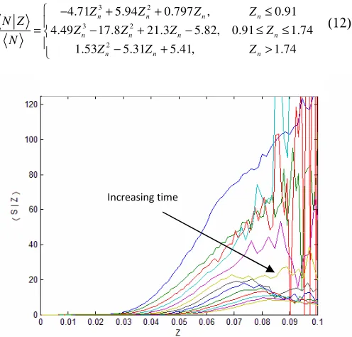
Figure 5. Conditional generation due to droplet formation versus mixture fraction over the life of the combustion.
Figure 6. The fit for conditional generation due to droplet formation at zone 0.
C. Conditional generation due to droplet formation
A plot of the conditional generation due to droplet formation, , versus mixture fraction for the length of combustion is shown in Fig. 5. This term refers to the contribution of the droplet evaporation to the gaseous phase of
the mass fraction of fuel. As can be seen from Fig. 5, the rate of generation due to droplet evaporation eases with time. This is because at the initial stage, the fuel vapour pressure is minimal, and there is a strong source of energy present in the form of the spark. The spark quickly evaporates the surrounding droplets and thus the generation is quite high. During the intermediate stage of combustion, the spark is deactivated, but combustion becomes self-sustained due to the advancement of the flame front. Again, evaporation is quite high and fuel is still being released to the system as a gas. However, the rate of evaporation becomes somewhat lower as the fuel is mixed through the air creating locations with relatively high mixture fraction but no droplets. In the final stage of combustion, the flame front is still providing energy for the evaporation of droplets, but the amount of droplets present to evaporate is small as most fuel has been expended in previous stages of the combustion.
Fig. 6 shows the fit for conditional generation due to droplet formation at zone 0. The equations describing the fit are shown in Eq. (13). Note that in this instance is not normalised.
5 3 4 2
0, 0.025
6.68 4.30
0.025 0.045 917 6.49,
1125 42.2, 0.04
1
5
0 10
Z
S Z Z Z
Z S Z Z Z ≤ − = ≤ ≤ + − − × >
× (13)
The fits to describe the conditional generation due to droplet formation for zones 1 to 3 is shown in Fig. 7. The fit for each curve is described with a composite function comprising an error function for low values of Z and linear fits for high values of Z. The error function fit is constant for all values of time while the gradient and position of the straight line varies with time.
Figure 7. The fits for normalised conditional generation due to droplet formation for zones 1 to 3.
The error function is defined as:
{
}
0.7 1 erf (38.9[ 0.0477]) .
S Z
Z
S = + −
[image:8.595.41.289.198.435.2] [image:8.595.312.555.458.632.2] [image:8.595.42.279.479.654.2]The coefficients of the straight lines are functions of time. Using a straight line of the form S Z S =m Z
(
−c)
, the values of and are shown below.3 2
3 2
2 60 58 6 458 0 1364 0 0001 0 0021 0 0172 0 0247
n n n
n n n
m . t + . t . t +
c . t . t + . t + .
= − −
= −
(15) (16) As can be seen, the error is greatest at the start of zone 1, and the fit becomes more accurate at the end of the combustion.
D. Chemical Source Term
The chemical source term can be approximated by an Arrhenius equation and is a function of the conditional mass fractions of fuel and air, and the conditional temperature. Because the CMC model solves for the mass fractions as well as temperature, can be calculated as the combustion proceeds.
IV. CONCLUSION
Modelling of combustion systems with the presence of droplets is very complicated because of the interaction of the evaporating liquid with the gaseous phase. The usage of a spark to evaporate the fuel and ignite the mixture exacerbates this complexity because the behaviour of the system is different to autoignition (which is the limiting behavior once the spark is deactivated). Because of this complex behavior which is not well understood, Direct Numerical Simulation (DNS) data have been analysed to provide models for terms and coefficients in the Conditional Moment Closure (CMC) model when droplets are present. Specifically, the
development of the mixture fraction probability density function (PDF), conditional scalar dissipation and conditional generation of fuel due to evaporation have been studied. Successful parameterisation of all the regimes due to the spark activation/deactivation has been performed. Future work includes: extension of the models to different initial conditions, validation of the models by simulating the DNS and implementation of the models to engineering-scale combustors.
REFERENCES
[1] Yoo, C. S., Sankaran, R. & Chen, J. H., “Three-dimensional direct numerical simulation of a turbulent lifted hydrogen jet flame in heated coflow: flame stabilization and structure”, Journal of Fluid Mechanics, vol. 640, pp. 453 – 481, 2009.
[2] Klimenko, A. Y. & Bilger, R.W., “Conditional moment closure for turbulent combustion”, Progress in Energy and Combustion Science, vol. 25, pp. 595 – 687, 1999.
[3] Wandel, A. P., Chakraborty, N. & Mastorakos, E., “Direct numerical simulations of turbulent flame expansion in fine sprays”, Proceedings of the Combustion Institute, vol. 32, pp. 2283 – 2290, 2009.
[4] Kim, I. S. & Mastorakos, E., “Simulations of turbulent non-premixed counterflow flames with first-order conditional moment closure”, Flow, Turbulence and Combustion, vol. 76, pp. 133 – 162, 2006.
[5] Wang, Y. & Rutland, C. J., “Direct numerical simulation of ignition in turbulent n-heptane liquid-fuel spray jets”, Combustion and Flame, vol. 149, pp. 353 – 365, 2007.
[6] Massebeuf, V., Bedat, B., Helie, J., Lauvergne, R., Simonin, O. & Poinsot, T. (2006), “Direct numerical simulation of evaporating droplets in turbulent flows for prediction of mixture fraction fluctuations: application to combustion simulations”, Journal of the Energy Institute, vol. 79, pp. 212 – 216, 2006.