This is a repository copy of Energy analysis and shadow modeling of a rectangular type salt gradient solar pond.
White Rose Research Online URL for this paper: http://eprints.whiterose.ac.uk/116444/
Version: Accepted Version
Article:
Aramesh, M, Kasaeian, A, Pourfayaz, F et al. (1 more author) (2017) Energy analysis and shadow modeling of a rectangular type salt gradient solar pond. Solar Energy, 146. pp. 161-171. ISSN 0038-092X
https://doi.org/10.1016/j.solener.2017.02.026
© 2017 Elsevier Ltd. This manuscript version is made available under the CC-BY-NC-ND 4.0 license http://creativecommons.org/licenses/by-nc-nd/4.0/.
[email protected] https://eprints.whiterose.ac.uk/ Reuse
Unless indicated otherwise, fulltext items are protected by copyright with all rights reserved. The copyright exception in section 29 of the Copyright, Designs and Patents Act 1988 allows the making of a single copy solely for the purpose of non-commercial research or private study within the limits of fair dealing. The publisher or other rights-holder may allow further reproduction and re-use of this version - refer to the White Rose Research Online record for this item. Where records identify the publisher as the copyright holder, users can verify any specific terms of use on the publisher’s website.
Takedown
If you consider content in White Rose Research Online to be in breach of UK law, please notify us by
1
Energy Analysis and Shadow Modeling of a Rectangular
1
Type Salt Gradient Solar Pond
2
3
Alibakhsh Kasaeian
1, Mohamad Aramesh
1,Fathollah Pourfayaz
14
Dongsheng Wen
2,35
6
1Faculty of New Science and Technologies, University of Tehran, Tehran, Iran.
7
2School of Chemical and Process Engineering, University of Leeds, Leeds, UK
8
3School of Aeronautic Science and Engineering, Beihang University, Beijing, PR China.
9
10
Abstract
11
In calculating the total solar energy input into a salt gradient solar pond, the current method was
12
incapable for use in long time periods and the calculation was imprecisefor sunny and shaded
13
areas.The existing relations of solar pond energy analysis can be used for momentary
14
calculations but it is very time-consuming forlong time periods. The shading effect inside the
15
pond affects significantly theenergy storage performance of the pond, especially in small ones.To
16
solve the first problem, the mean values of variable parameters during the time periods is
17
proposed in this work and the ‘first mean value theorem for definite integrals’ is used for
18
deriving the averageof those parameters. For the second problem,a rectangular pond with vertical
19
walls is investigated, and the exact sunny areas in different depths of the pondare calculated at
20
different time conditions. The experimental data of a previously worked paper is used for
21
validation. The energy efficiency of the low convective zone of the experimental pond is
2
calculated theoretically, and the results show that the theoretical and experimental values are in
23
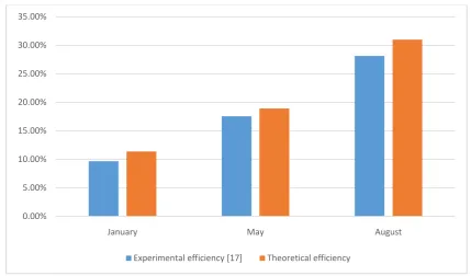
good agreement with each other. The experimental data and theoretical results for the energy
24
efficiency are 9.68% and 11.38% for January, 17.54% and 18.92% for May and 28.11% and
25
30.94% for August,respectively. Therefore, the modified relations can be a good reference for
26
predicting a pond performance before its construction.
27
28
Keywords: Salt gradient solar pond; Energy analysis; Shadow effect.
29
30
1. Introduction
31
With increasing concerns of carbon emission and global warming, there is an urgent need to
32
developalternative energy sources to replace fossil fuels in the long term[1]. Developing
33
renewable energy technologies,especially solar-based,has received intensive interest in the last a
34
few decades[2, 3]. Among present technologies for various applications of solar energy, salt
35
gradient solar pond is a promising optionfor solar energy storage due to its unique characteristics
36
such as low cost and high capability for long-term energy storage[4-6]. Many studieshave been
37
conductedon the energy analysis of solar pond in different conditions for the purpose of
38
optimization[7], which is briefly reviewed below.
39
Jafarzade[8] studied the thermal behavior of a small salt gradient solar pond with wall shading
40
effect in 2004.The effect of vertical walls of a square pond on the reduction of the sunny area
41
was included in the model, and theresult reported an overall efficiency of 10% for the pond. In
42
2006 Karalikick et al. [9] presented an experimental and theoretical investigation of temperature
43
distributions in an insulated solar pond during both daytime and night time. Theoretical
3
temperature distributions were compared withvarious cases, such as inside the pond, underneath
45
the pond and in the side walls.
46
In 2008 Karakilicik et al.[10] presented an experimental and theoretical investigation of
47
exergyperformance of a solar pond. The exergy efficiencies were less than the energy
48
efficiencies for each zone of the pond due to the exergy destructions in the zones and losses to
49
the surroundings. Bozkurt et al. [11]presented a heat storage performance investigation of an
50
integrated solar pond with a collector system in 2012. It was concluded that to increase
51
thesystem performance, the zone thicknesses, sunny areas of the pond, number of the collectors
52
and salt gradient system should be modified to achieve higher efficiency and stability of the
53
pond.In the same year, Bozkurt et al. [12]compared the performance of an integrated and a
54
nonintegrated solar pond experimentally, and revealed a higherenergy efficiency for the
55
integrated system.
56
In 2013 Karakilcik et al.[13] presented an experimental investigation of the energy distribution
57
and energy efficiency of a small rectangular solar pond due to shading effect on each zone, and
58
found that the efficiency of the solar pond was decreasedby increasing the shading area.Atiz et
59
al.[14] in 2014 studied the turbidity effect on the exergy performance of solar ponds under
60
various weather conditions and concentrations. The results showed that the exergyefficiency
61
wassignificantly decreased by increasing the turbidities of the zones. In the same year, Bozkurt et
62
al.[15] presented a theoretical analysis for a solar pond at different geometries for the Adiyaman
63
region in Turkey.The energy efficiency of the solar pond was increased by an increase in the size
64
of the pond. In 2015, Bozkurt et al.[16] presented a new performance model to determine the
65
energy storage efficiency of a solar pond.The heat losses of the solar pond were determined by
66
using the Heat 2 software. The experimental and the theoretical heat storage performance of the
4
lower convective zone of the solar pond were determined, and the results showed that the
68
presented model could predict the efficiency of the pond with a good accuracy.In 2015, Bozkurt
69
et al.[17]investigated the effect of the sunny area ratios on the thermal efficiency of a solar pond
70
model. The results showed that with an increase of sunny area ratio, the performance of the solar
71
pond was increased. Another research by Bozkurt et al.[18] in 2015 studied the performance of a
72
magnesium chloride saturated solar pond. The maximum energy and exergy efficiencies
73
werefound to be respectively 27.41% and 26.04% for the heat storage zone in August.
74
In all previous studies, the existing equations could be used for the momentary time intervals, but
75
a massive amount of calculations was needed to analyze the energy behavior of solar ponds
76
during a specific period. Moreover, in the previous works, the walls` shading effect was either
77
neglected or was not considered precisely. In this study, the energy analysis of solar pondsis
78
modified for the first time, to eliminate the mentioned drawbacks of previously used methods.
79
The average value of variable parameters are implemented in the modified method, which can be
80
used to calculate the pond performance for a much longer period, yet with much less
81
calculations. .In addition, accurate correlations are presented for rectangular ponds to obtain the
82
exact sunny areas inside the pond in different time and locations. The presented energy analysis
83
method shows better accuracy than the former methods in predicting the behavior of a pond.
84
85
2. Energy Analysis
86
In the correlations for calculating the amount of solar energy entering the pond at different pond
87
depths, various parameters are dependent on the sun incident angle. It is very time consuming in
88
considering the changes of this angle during a day and different seasons in order to find the total
89
amount of the entered energy. A simplification of these correlations can lead to less amount of
5
calculations. In next sections, the principles of this study will be described and then modification
91
of the relations will be discussed.
92
2.1. Principles 93
The equation that is being used widely to calculate the energy entering the pond in any depth is
94
given by [19, 20]:
95
(1)
= ℎ( )
where is the total solar energy flux reaching pond surface ( ), is the fraction of the incident
96
solar radiation that enters the pond, is the sunny area of solar pond at the desired depth of
97
( ), and ℎ( ) is the ratio of the solar energy reaching to that depth. The value of can be
98
measured during the desired period or can be inquired from meteorological stations.
99
The parameters of , and ℎ are dependent on the incident angle of solar irradiance to the pond.
100
Therefore Eq. (1) can calculate entering energy to the pond only in short periods of time in which
101
the incident angle can be considered as a constant. On the other hand, for rectangular solar ponds,
102
the azimuth angle can also affect the sunny areas inside the pond, as a change in azimuth angle
103
changes the walls shading. In the previous studies, which considered the shading effect, solar
104
pond direction is assumed to be in a way that the azimuth angle become equal to zero and the
105
shading is limited to only one of the walls [13, 17, 21]. By considering the changes in the
106
azimuth angle during the day, this assumption is valid only for short periods of time. In order to
107
solve the mentioned problems, the equations of those three parameters must be modified. In the
108
first case, the equations must be modified to calculate the solar energy entering the pond at
109
different time intervals. For the second case, the equations must be modified so that the exact
110
sunny area of the pond at different depths and time intervals could be calculated.
6
To calculate the amount of energy entering the pond at any time intervals, Eq. (1) can be written
112
in the integral form as followings:
113
, = ℎ( )
,
,
(2)
And by taking out the parameters that are independent of the incident angle from the integral:
114
, = ℎ
,
,
(3)
In these equations, is time dependent, and it is calculated by multiplying solar irradiance,
115
(which is usually given in / or ⁄ℎ . ) into the time of calculations. Since the
116
analytical solution of the three parameters in the integral is so complicated, a numerical solution
117
could be a wiser option. On the other hand by considering a mean value for any of the three
118
parameters in the desired period, the value of , in that period can be calculated using the
119
mean values of those parameters. Therefore, in this case, Eq. (1) can be transformed to Eq. (4):
120
= ̅ ℎ( ) (4)
where ̅, and ℎ are the mean values of , and ℎ in the specified period,respectively. For the
121
purpose of finding the mean values of these parameters, the method of first mean value theorem
122
for definite integrals can be used. Based on this theorem, the mean value of a function in a
123
particular range of its variable is equal to the area under the function curve divided by length of
124
variable range [22]:
125
7
Based on this method, modified equations of the mentioned parameters are presented in this
126
paper. In the next sections, parameters of ,ℎ and will be discussed, respectively.
127
128
2.2. Modifying equation 129
By considering previous studies, the value of is given by [19, 20]:
130
= 1 − 0.5 sin ( − )sin ( + )+tan ( − )tan ( + ) (6)
where is the incident angle and is the refraction angle. According to the complex relation of
131
, the analytical integration of this parameter needs complicated mathematical processes.To find
132
a relation forthe integration of parameter, this parameter can be plotted for all possible values
133
of incident angle (0 to 90 degrees), and an equivalent polynomial can be achieved for it, using
134
curve fitting methods. To do the fitting, it is needed to eliminate , which is a function of ,
135
from Eq. (6). The relation between these two parameters can be written using theSnell's Lawas
136
followings[23]:
137
sin( ) = sin( ) (7)
where and are refraction indexes of first and second media.Here these media are air and
138
water and their refraction indexes are equal to 1.0000 and 1.3330, respectively. Thus, the relation
139
between the two angles would be as followings:
140
sin( ) =1.00001.3330 sin( ) = 0.75 sin( ) (8)
Furthermore:
8
= sin (0.75 sin( )) (9)
Therefore, value of can be replaced with sin (0.75 sin( )):
142
= 1 − 0.5 sin ( − sin (0.75 sin( )))sin ( + sin (0.75 sin( )))+tan ( − sin (0.75 sin( )))tan ( + sin (0.75 sin( ))) (10)
It must be noted that in common solar ponds, the operating fluidsare water anddifferent solutions
143
of salt and water. Some exceptions may use other fluids, thus, in such cases the value of the
144
refraction angle must be calculated using Eq. (7) and the proper value must be used in further
145
equations. Also this value changes with increase of salt concentration, but this difference is small
146
and can be generally neglected. So it can be assumed that the value of the refraction anglein all
147
the layers of the pond is equal to that of the pure water.
148
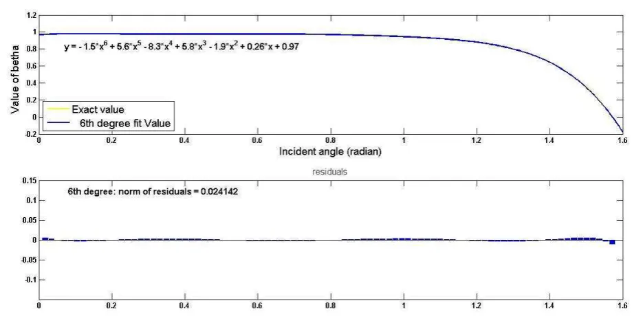
Using Eq. (10), values of have been plotted based on values of (in radian), and its curve has
149
been fitted using MATLAB software. Fig. 1 shows the curve fitting results.
150
[image:9.595.65.525.446.681.2]151
Fig. 1. The difference between values of using the original equation and the fitted equation in
152
all incident angles.
9
The fitted equation of this parameter, which can calculate the value of with less than 1% error,
154
is as followings:
155
= −1.5 + 5.6 − 8.3 + 5.8 − 1.9 + 0.26 + 0.97 (11)
where is in radian form. Hence, the integral of this parameter can be calculated using following
156
equation:
157
= −143 +1415 −5088 +2920 −1930 + 0.13 + 0.97 + (12)
The parameter of is the integral constant and value of it is not a concern in definite integrals.
158
Therefore, the mean value of can be calculated using Eqs. (5) and (12). It must be noted that
159
according to the definition of the incident angle, if this angle reaches to zero in the desired
160
interval, the mean value must be calculated using the equation below:
161
̅ =∫ , + ∫ ,
, − 0 + , − 0
(13)
162
2.3. Modifying ℎ equation 163
Value of ℎ can be calculated by Eq. (14)[19, 20]:
164
ℎ = 0.36 − 0.08 ( ) (14)
where is the desired depth (m). Considering theSnell's Law and the logarithm function
165
characteristics:
10
ℎ = 0.36 − 0.08[ ( ) − ( ( (0.75 ( ))))]
= 0.36 − 0.08 ( ) + 0.08[ ( ( (0.75 ( ))))] (15)
167
Eq. (15) calculates the value of ℎ as a function of the incident angle. Analytical integration of
168
this equation results in complex numbers. Likewise, the parameter of , integral of this
169
parameter can be calculated using curve fitting methods. It must be noted that the second term in
170
the right-hand side (−0.08 ln( )) is not a function of the incident angle. Thus, for every depths,
171
this parameter can be considered as a constant value. Using MATLAB software and Eq. (15), the
172
fitted equation ofℎ − (−0.08 ln( ))is as followings:
173
ℎ + 0.08 ( ) = 0.0104 − 0.0156 − 0.0132 − 0.0019 + 0.3601 (16)
Then, the relation of ℎ can be written as Eq. (17):
174
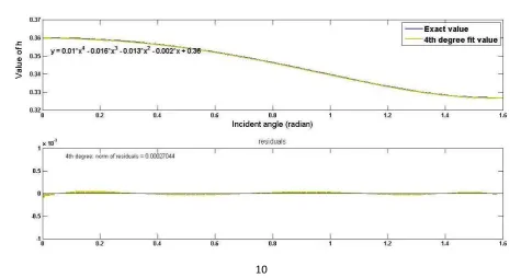
[image:11.595.59.525.506.760.2]ℎ = 0.0104 − 0.0156 − 0.0132 − 0.0019 + 0.3601 − 0.08 ( ) (17)
Fig. 2 shows the accuracy of Eq. (16) for calculating the value of ℎ − (−0.056 ln( )).
175
11
Fig. 2. The difference between values ofℎ + 0.08 ln( ) using the original equation and the
177
fitted equation in all incident angles.
178
Eq. (17) is the result of adding the same constant value to both sides of Eq. (16). Therefore, the
179
accuracy of Eq. (17) is the same with Eq. (16) and theerror percentage for calculating theℎ
180
parameterusing Eq. (17) will be less than 0.02%. In the fitting processes for both parameters of
181
and ℎ, the incident angle was taken in the radian form, so this parameter in the polynomial
182
equations must be used in the radian form too. Also, the values of the incident angle have been
183
shown in the radian form in Figs. 1 and 2. Integration of Eq. (17) results in the following
184
equation:
185
ℎ = 0.0020 − 0.0040 − 0.0043 − 0.0010
+ (0.0400 − 0.08 ( )) +
(18)
Similar to Eq. (12), it is not needed to calculate the integral constant in Eq. (18). Therefore, the
186
mean value of ℎ can be calculated using Eqs. (5) and (18). As it was mentioned before, if there is
187
zero incident angle in the interval, the mean value of ℎ can be calculated as followings:
188
ℎ =∫ ℎ
, + ∫ ℎ,
, − 0 + , − 0
(19)
189
2.4. Calculating exact sunny areas 190
The sunny area of the pond influencesthe solar energy absorbance [17]. By taking into account
191
the shading of the pond walls, this area is less than the pond cross section. Therefore, to increase
192
the accuracy of the calculations, the shading effect must be studied. In this study rectangular
12
ponds with vertical walls have been investigated. In this type of ponds, the azimuth angle is
194
effective on the walls shading as well as the incident angle. Thus in the next sections firstly the
195
incident and azimuth angles will be discussed and then the proper relations for calculating the
196
sunny areas for this type of ponds will be presented.
197
198
Solar angles 199
In previous studies on the rectangular ponds, only one of the pond’s walls were considered to be
200
effective on the shading [8, 13, 17, 21]. This situation would occur only in a short periods
201
because the direction of the solar incident to the pond will vary with the changes in the azimuth
202
angle during the day and various shaded areas will be expected. Thus, to calculate the sunny
203
areas, the effects of the bothincident and azimuth angles must be considered. These angles are
204
dependent on time and location. The value of the incident angle can be calculated using Eq.
205
(20)[23]:
206
cos( ) = sin( ) sin( ) cos( ) − sin( ) cos( ) sin( ) cos( )
+ cos( ) cos( ) cos( ) cos( ) + cos( ) sin( ) sin( ) cos( ) cos( )
+ cos( ) sin( ) sin( ) sin( )
(20)
where is the declination angle, is the latitude, is the tilt angle of the pond’s surface, is the
207
surface azimuth angle and is the hour angle. Solar ponds are not tilted, and their surface is
208
horizontal, so the tilt angle is equal to zero. Therefore, the incident angle can be calculated using
209
the equation below:
210
13
The solar azimuth angle for horizontal surfaces can be found using the following equation [23]:
211
= ( ) ( ) ( )( ) −( ) ( ) (22)
where ( ) is the sign function of the hour angle. Fig. 3 schematically describes , , and
212
angles.
213
214
[image:14.595.138.461.282.619.2]215
Fig. 3. Schematics of the tilt, surface’s azimuth, solar azimuth and incident angles[23]
216
14
Here it has been assumed that one of the pond walls is facing to the south, so based on Fig. 3,
218
only the solar azimuth angle effects on shadow creation. In other circumstances, the summation
219
of the solar and surface azimuth angles must be used for calculations.
220
As it can be seen in Eqs. (21) and (22), the effective angles on the incident and azimuth angles
221
are , and . The angle that represents the latitude, can be determined by the location of the
222
pond. The other two angles can be calculated by their relations. Eq. (23) shows the relation for
223
the declination angle[24]:
224
= 23.44 360365.25− 80 (23)
where is the day number and for the latitudes below 66.5 degrees, this parameter can be defined
225
using Table 1. [25]:
[image:15.595.177.417.456.753.2]226
Table 1. Number of days in a year
227
Month Date Day number
January 1st 1
February 1st 32
March 1st 60
April 1st 91
May 1st 121
June 1st 152
15
August 1st 213
September 1st 244
October 1st 274
November 1st 305
December 1st 335
228
Also, the hour angle can be calculated using following equation[24]:
229
=86400360 ( − 43200) (24)
where is the local solar time in seconds. To calculate solar local time the equation below can be
230
used [23]:
231
− = 4( − ) + (25)
where standard time is equal to the clock time in the standard local meridian of the pond's
232
location, is the standard local meridian longitude, is the longitude of the pond's location,
233
and is the equation of time. It should be mentioned that all the time units in Eq. (25) are in
234
minutes. To use the value of in Eq. (24), conversion to the second unit must be considered. The
235
value of in minutes can be calculated using Eq. (26) [24].
236
= −0.017188 − 0.42811 ( ) + 7.35141 ( ) (26)
where is the representation of the day number in angle and is defined as followings[24]:
16
=360365 (27)
Therefore through Eqs. (23) to (27) and considering the latitude of pond's location, the incident
238
angle can be calculated by Eq. (21), and the solar azimuth angle can be foundusing Eq. (22).
239
The azimuth angle determines the shape of the shadow and incident angle specifiesits size. This
240
is shown schematically in Fig. 4.
241
[image:17.595.63.510.276.423.2]242
Fig. 4. Effect of the azimuth angle on the shape of the shadow
243
244
In this figure, the red rectangle represents the solar radiation area, and the black rectangle
245
represents the solar pond's cross section. The gray surfaces are shaded areas, and the white
246
surfaces are the sunny areas. Hypothetical solar radiation area moves towards left or right by the
247
changes in the value of azimuth angle.It can be concluded from Eqs. (21) to (27) that both
248
incident and azimuth angles are functions of time. Therefore to calculate sunny areas inside the
249
pond, calculations must be performed during the desired period. This can be considered for other
250
parts of this paper since incident angle was introduced as a reference for former calculations
251
while incident angle itself is a function of time.
17
By defining the basics, calculation of sunny areas in the ponds with rectangular cross sections
253
will be discussed in the next section.
254
Solar ponds with rectangular cross section and vertical walls 255
To find sunny areas in these types of ponds, trigonometric and geometric relations must be
256
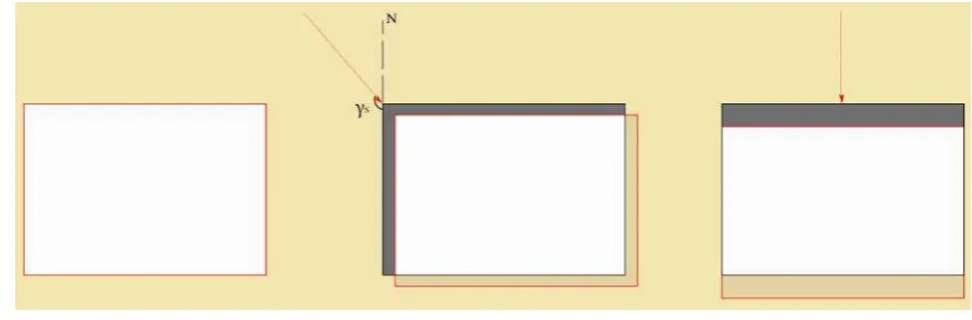
considered. Fig. 5 reveals the relations between the created shadow and azimuth and incident
257
angles. It must be noted that the refraction angles of azimuth and incident angles cause creating
258
the shadow and the refraction angles will be used in calculations. Also, the size of the shadow
259
inside the pond in different depths is only affected by incident refraction angle. Moreover,
260
azimuth refraction angle just determines the shape of the shadow.
261
18
Fig. 5. Effects of azimuth angle on shape of the shadow
263
In Fig. 5, coordinate axes which represent geographical orientations are shown with blue color,
264
sunlight beam is shown by red color, sunny area in the depth of ′ is demonstrated by white color
265
and shadow area in that depth is indicated by gray color. Considering geometric relations, ratios
266
of , and , which form solar radiation vector, remain constant and can be described as
267
followings:
268
= ′′ , = ′ , =′ ′′ (28)
Therefore for any desired depth such as ′, and can be calculated considering solar radiation
269
vector components. The ratios between these components are dependent to the refraction angles
270
of incident and azimuth angles:
271
= = ⇒ = (29)
= = ⇒ = ⇒ = (30)
Using Eqs. (29) and (30), for any given depth of the pond, shadow thickness can be determined
272
in and directions respectively. To calculate the sunny area, the shadow area must be
273
subtracted from the cross section of the pond. Considering as length of the pond (north to south
274
direction) and as width of the pond (east to west direction), due to Fig. 5, following equation,
275
can be written:
19
= ( × ) − ( − ) + ( − ) + ( × )
= − ( + − ) = + − −
(31)
Using Eqs. (29) and (30), Eq. (31) can be rewritten as followings:
277
= + ( ) − − (32)
This parameter is a function of incident refraction angle and depth of the pond. Hence, it needs
278
two averaging steps to find the mean value in the desired layer and in desired time interval.
279
According to the complicated relations of this parameter, numerical methods are proper ways for
280
calculation of the mean values.
281
Thereupon calculation of sunny areas, as well as other parameters in energy relations, were
282
discussed. Using mean values of these parameters in Eq. (4), the solar energy entering the pond
283
can be calculated precisely which will be discussed in next section.
284
285
3. Results and Discussion
286
In this section, before investigating the modified relations, the shading effect will be studied. To
287
do so, dimensions of an experimental salt gradient solar pond constructed in Adiyaman, Turkey,
288
have been considered [17, 21, 26]. The dimensions are mentioned in Table 2.
289
290
291
Table 2. Characteristics of the experimental pond [17, 21, 26].
20
Pond’s depth Pond’s length Pond’s width UCZ thickness NCZ thickness LCZ thickness
1.5 m 2 m 2 m 0.1 m 0.6 m 0.8 m
293
294
Also, four different location and time condition combinations have been assumed which are
295
shown in Table 3.
296
297
[image:21.595.69.527.142.177.2]298
Table 3. Location and time conditions
299
Condition City (latitude)
Day’s
number-Date
(Declination
angle)
Time
(hour
angle)
Refraction
angle
Azimuth
angle
Con. 1 Tehran (+35.6961º) 217-August 6
th
(16.57º)
8
(-60º) 56.2479º -47.2507º
Con. 2 Tehran (+35.6961º)
217-August 6th
(16.57º)
12
(0º) 19.1261º -2.7046º
Con. 3 Tehran (+35.6961º)
35-feburary 4th
(-16.39º)
8
21
Con. 4 Singapore (+1.3000º) 217-August 6
th
(16.57º)
8
(-60º) 69.9493º 39.9614º
[image:22.595.39.521.85.700.2]300
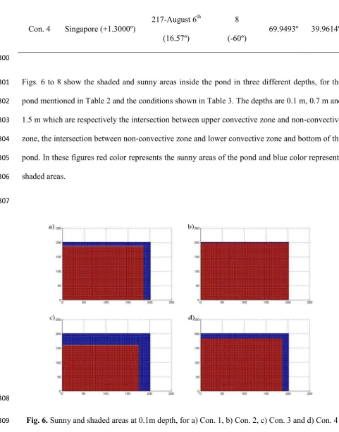
Figs. 6 to 8 show the shaded and sunny areas inside the pond in three different depths, for the
301
pond mentioned in Table 2 and the conditions shown in Table 3. The depths are 0.1 m, 0.7 m and
302
1.5 m which are respectively the intersection between upper convective zone and non-convective
303
zone, the intersection between non-convective zone and lower convective zone and bottom of the
304
pond. In these figures red color represents the sunny areas of the pond and blue color represents
305
shaded areas.
306
307
308
Fig. 6. Sunny and shaded areas at 0.1m depth, for a) Con. 1, b) Con. 2, c) Con. 3 and d) Con. 4
[image:22.595.103.485.397.658.2]22 310
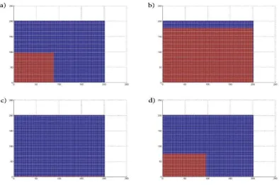
Fig. 7. Sunny and shaded areas at 0.7m depth, for a) Con. 1, b) Con. 2, c) Con. 3 and d) Con. 4
311
23
Fig. 8. Sunny and shaded areas at 1.5m depth, for a) Con. 1, b) Con. 2, c) Con. 3 and d) Con. 4
313
Figs. 6 to 8 show that the shadow created inside the pond can have a significant effect on the
314
energy absorbed inside the pond. For a better understanding of shadow effects, the sunny areas
315
of each case in all of the considered conditions have been calculated and are presented in terms
316
of sunny volume ratios in Table 4. These ratios show the sunny volume of the pond to its total
317
volume.
318
319
Table 4. Sunny volume ratios of the pond in all considered cases and conditions
320
Parameter Con. 1 Con. 2 Con. 3 Con. 4
Sunny area volume 0.3285 0.6013 0.2987 0.7213
321
According to the direct effect of sunny areas in energy relations, these values show that
322
neglecting the shading effect can lead to high errors in calculations.
323
In the next part of results, the accuracy of modified equations will be studied. For this purpose,
324
one of the previous experimental studies on solar pond energy analysis will be considered as a
325
reference. Karaklick et al.(2006) presented an experimental study on a salt gradient solar pond in
326
the city of Adiyaman in Turkey. Experimental data of this pond are given in three different
327
studies [17, 21, 26]. Dimensions of the pond have been mentioned in Table 2, and the
energy-328
related data are shown in Table 5.
329
24
Table 5. Experimental data for heat stored in LCZ layer and solar irradiance
331
parameter August May January
. ( ) 252.65 160.31 18.7
( ⁄ ) 690 713 175
332
The LCZ layer efficiency has been calculated using following equation [26]:
333
= .
, (33)
where is the thermal efficiency of LCZ layer, . is the amount of energy which is
334
stored in LCZ layer and , is the amount of solar radiation heat which enters this layer
335
and can be calculated using modified relations in this article. Using those relations and
336
experimental data, the energy efficiency of LCZ layer has been calculated theoretically. The
337
theoretical and experimental results are shown in Table 6.
338
339
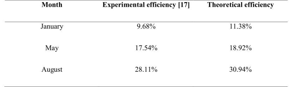
Table 6. Comparison of theoretical and experimental energy efficiencies of LCZ layer
340
Month Experimental efficiency [17] Theoretical efficiency
January 9.68% 11.38%
May 17.54% 18.92%
August 28.11% 30.94%
[image:25.595.57.522.581.721.2]25
These results are shown graphically in Fig. 9.
342
[image:26.595.82.512.136.388.2]343
Fig. 9. Graphical comparison of theoretical and experimental energy efficiencies of LCZ layer
344
The results reported inTable 6 and Fig. 9 show that the theoretical efficiencies are in good
345
agreement with the experimental values. Therefore, this method can predict the values of energy
346
entering the pond or energy efficiencies of different layers with a good accuracy.
347
348
4. Conclusion
349
In this paper, a modified modelingmethod for calculating solar energy entering a salt gradient
350
solar pond and its layers was presented. In the former studies there are two primary limitations:
351
1. Existing parameters in equations are dependent on the solar incident angle, which varies with
352
time, and the relations can calculate energies only in short periods of time.
353
0.00% 5.00% 10.00% 15.00% 20.00% 25.00% 30.00% 35.00%
January May August
26
2. The shading effectinside the pound, which has a significant impact on the value of energy
354
entering the pond, wasneglected or calculated insufficiently.
355
The present study deals with the first issue by using mean values of the parameters during the
356
considered time interval. The expressions for parameters of (i.e., the fraction of solar radiation
357
which enters the pond) and ℎ (i.e., the fraction of total solar energy which reaches to desired
358
depth) were presented. Then, to deal with the second issue, rectangular solar ponds with vertical
359
walls were considered, and proper equations for calculating exact values for sunny areas were
360
presented.
361
The results from modified equations were compared with a published experimental study and
362
good agreement was found. . The theoretically predicted efficiencies for LCZ layer had 1.7%,
363
1.38% and 2.83% differences with experimental data for the months of January, May and August
364
respectively. Therefore, this method can be used to predict the amount of energy entering the
365
pond or energy efficiency for different layers of it with a good accuracy. For practical
366
applications,these governing parameters can be easily calculated before building a specified solar
367
pond and the dimensions of it can be optimized to reach a designed outcome.
368
369
Refrences 370
371
[1] A.M.K. Vandani, M. Bidi, F. Ahmadi, Exergy analysis and evolutionary optimization of boiler 372
blowdown heat recovery in steam power plants, Energy Conversion and Management, 106 (2015) 1-9. 373
[2] A. Sakhrieh, A. Al-Salaymeh, Experimental and numerical investigations of salt gradient solar pond 374
under Jordanian climate conditions, Energy Conversion and Management, 65 (2013) 725-728. 375
[3] R. Boudhiaf, M. Baccar, Transient hydrodynamic, heat and mass transfer in a salinity gradient solar 376
pond: A numerical study, Energy Conversion and Management, 79 (2014) 568-580. 377
[4] Z. Hongfei, J. Hua, Z. Lianying, W. Yuyuan, Mathematical model of the thermal utilization coefficient 378
27
[5] M. Husain, P.S. Patil, S.R. Patil, S.K. Samdarshi, Combined effect of bottom reflectivity and water 380
turbidity on steady state thermal efficiency of salt gradient solar pond, Energy Conversion and 381
Management, 45 (2004) 73-81. 382
[6] H. Kurt, F. Halici, A.K. Binark, Solar pond conception — experimental and theoretical studies, Energy 383
Conversion and Management, 41 (2000) 939-951. 384
[7] M. Husain, S.R. Patil, P.S. Patil, S.K. Samdarshi, Simple methods for estimation of radiation flux in 385
solar ponds, Energy Conversion and Management, 45 (2004) 303-314. 386
[8] M.R. Jaefarzadeh, Thermal behavior of a small salinity-gradient solar pond with wall shading effect, 387
Solar Energy, 77 (2004) 281-290. 388
[9] M. Karakilcik, K. Kıymaç, I. Dincer, Experimental and theoretical temperature distributions in a solar 389
pond, International Journal of Heat and Mass Transfer, 49 (2006) 825-835. 390
[10] M. Karakilcik, I. Dincer, Exergetic performance analysis of a solar pond, International Journal of 391
Thermal Sciences, 47 (2008) 93-102. 392
[11] I. Bozkurt, M. Karakilcik, The daily performance of a solar pond integrated with solar collectors, 393
Solar Energy, 86 (2012) 1611-1620. 394
[12] I. Bozkurt, M. Karakilcik, I. Dincer, Energy efficiency assessment of integrated and nonintegrated 395
solar ponds, International Journal of Low-Carbon Technologies, 9 (2012) 45-51. 396
[13] M. Karakilcik, I. Dincer, I. Bozkurt, A. Atiz, Performance assessment of a solar pond with and without 397
shading effect, Energy Conversion and Management, 65 (2013) 98-107. 398
[14] A. Atiz, I. Bozkurt, M. Karakilcik, I. Dincer, Investigation of turbidity effect on exergetic performance 399
of solar ponds, Energy Conversion and Management, 87 (2014) 351-358. 400
[15] I. Bozkurt, A. Atiz, M. Karakilcik, I. Dincer, Performance Analysis of a Solar Pond, in: I. Dincer, A. 401
Midilli, H. Kucuk (Eds.) Progress in Exergy, Energy, and the Environment, Springer International 402
Publishing, Cham, 2014, pp. 783-790. 403
[16] I. Bozkurt, S. Mantar, M. Karakilcik, A new performance model to determine energy storage 404
efficiencies of a solar pond, Heat Mass Transfer, 51 (2015) 39-48. 405
[17] I. Bozkurt, M. Karakilcik, The effect of sunny area ratios on the thermal performance of solar ponds, 406
Energy Conversion and Management, 91 (2015) 323-332. 407
[18] I. Bozkurt, S. Deniz, M. Karakilcik, I. Dincer, Performance assessment of a magnesium chloride 408
saturated solar pond, Renewable Energy, 78 (2015) 35-41. 409
[19] I. Bozkurt, Reply to “Erroneous equations used to assess the performance of a solar pond” by 410
Morteza Khalilian, Energy Conversion and Management, 114 (2016) 399. 411
[20] M. Khalilian, Erroneous equations used to assess the performance of a solar pond, Energy 412
Conversion and Management, 114 (2016) 394-398. 413
[21] I. Dincer, M.A. Rosen, EXERGY: Energy, Environment and Sustainable Development, Elsevier Science, 414
2012. 415
[22] R.C. James, G. James, The Mathematics Dictionary, Springer Netherlands, 1992. 416
[23] W.A.B. John A. Duffie, Solar Engineering of Thermal Processes, 4th Edition, New York, 2013. 417
[24] A.V. da Rosa, Fundamentals of Renewable Energy Processes (Third Edition), Academic Press, Boston, 418
2012. 419
[25] S.A. Klein, Calculation of monthly average insolation on tilted surfaces, Solar Energy, 19 (1977) 325-420
329. 421
[26] M. Karakilcik, I. Dincer, M.A. Rosen, Performance investigation of a solar pond, Applied Thermal 422
Engineering, 26 (2006) 727-735. 423
![Fig. 3. Schematics of the tilt, surface’s azimuth, solar azimuth and incident angles[23]](https://thumb-us.123doks.com/thumbv2/123dok_us/7727385.161996/14.595.138.461.282.619/fig-schematics-surface-azimuth-solar-azimuth-incident-angles.webp)