Characterising particulate random media from near-surface backscattering: A machine learning approach to predict particle size and concentration

This is a repository copy of

Characterising particulate random media from near-surface

backscattering: A machine learning approach to predict particle size and concentration

.

White Rose Research Online URL for this paper:

http://eprints.whiterose.ac.uk/147117/

Version: Published Version

Article:

Gower, A.L. orcid.org/0000-0002-3229-5451, Gower, R.M., Deakin, J. et al. (2 more

authors) (2018) Characterising particulate random media from near-surface

backscattering: A machine learning approach to predict particle size and concentration.

EPL, 122 (5). 54001. ISSN 0295-5075

https://doi.org/10.1209/0295-5075/122/54001

[email protected] https://eprints.whiterose.ac.uk/ Reuse

This article is distributed under the terms of the Creative Commons Attribution (CC BY) licence. This licence allows you to distribute, remix, tweak, and build upon the work, even commercially, as long as you credit the authors for the original work. More information and the full terms of the licence here:

https://creativecommons.org/licenses/

Takedown

If you consider content in White Rose Research Online to be in breach of UK law, please notify us by

LETTER • OPEN ACCESS

Characterising particulate random media from

near-surface backscattering: A machine learning

approach to predict particle size and concentration

To cite this article: Artur L. Gower et al 2018 EPL 122 54001

View the article online for updates and enhancements.

Related content

Ultrasound techniques for characterizing colloidal dispersions

R E Challis, M J W Povey, M L Mather et al.

-Equivalence between three scattering formulations for ultrasonic wave propagation in particulate mixtures

R E Challis, J S Tebbutt and A K Holmes

-Coherent backscattering of

electromagnetic waves in random media

A. Sheikhan, P. Maass and M. Reza Rahimi Tabar

-June 2018

EPL,122_{(2018) 54001} www.epljournal.org

doi: 10.1209/0295-5075/122/54001

Characterising particulate random media from near-surface

backscattering: A machine learning approach to predict particle

size and concentration

Artur L. Gower1, Robert M. Gower2, Jonathan Deakin1, William J. Parnell1andI. David Abrahams3

1 _{School of Mathematics, University of Manchester - Oxford Road, Manchester, M13 9PL, UK} 2 _{LTCI, T´el´ecom Paristech, Universit´e Paris-Saclay - 75013, Paris, France}

3 _{Isaac Newton Institute for Mathematical Sciences - 20 Clarkson Road, Cambridge, CB3 0EH, UK}

received 6 April 2018; accepted in final form 23 June 2018 published online 18 July 2018

PACS 42.25.Dd– Wave propagation in random media PACS 43.20.Fn– Scattering of acoustic waves PACS 05.10.Ln– Monte Carlo methods

Abstract _{– To what extent can particulate random media be characterised using direct wave} backscattering from a single receiver/source? Here, in a two-dimensional setting, we show using a machine learning approach that both the particle radius and concentration can be accurately measured when the boundary condition on the particles is of Dirichlet type. Although the methods we introduce could be applied to any particle type. In general backscattering is challenging to interpret for a wide range of particle concentrations, because multiple scattering cannot be ignored, except in the very dilute range. Across the concentration range from 1% to 20% we find that the mean backscattered wave field is sufficient to accurately determine the concentration of particles. However, to accurately determine the particle radius, the second moment, or average intensity, of the backscattering is necessary. We are also able to determine what is the ideal frequency range to measure a broad range of particles sizes. To get rigorous results with supervised machine learning requires a large, highly precise, dataset of backscattered waves from an infinite half-space filled with particles. We are able to create this dataset by introducing a numerical approach which accurately approximates the backscattering from an infinite half-space.

open access Copyright cEPLA, 2018

Published by the EPLA under the terms of the Creative Commons Attribution 3.0 License (CC BY). Further distribution of this work must maintain attribution to the author(s) and the published article’s title, journal citation, and DOI.

Under close inspection, many materials are composed of small randomly distributed particles or inclusions. So it is no surprise that the need to measure particle properties, such as their average size and concentration, spans many physical disciplines. For quick non-invasive measurements, waves, either mechanical, electromagnetic or quantum, are the preferred choice. However, measuring a broad range of particle concentrations and sizes is still an open challenge. For high concentrations the wave undergoes multiple scat-tering, which requires specialised methods to compute and interpret. And further, measuring a wide range of parti-cle sizes means a wide range of frequencies needs to be considered.

The type of wave used depends on the type of particle: acoustic waves are used to measure liquid emulsions [1], sediment on the ocean floor [2] and polycrystalline ma-terials [3]. Microwaves are vital in remote sensing of

ice [4]; optics for aerosols [5] and cellular components, both micrometer [6] and nanoscale [7] structures, among many other applications. In all these applications, there are cases when transmission experiments are impractical, because either the material is too opaque or, for example, has an unknown depth. The next natural choice is to use reflected, orbackscattered, waves.

Here we ask: can one source/receiver measure the prop-erties of a random particulate medium? And is it possible to do so without measuring the backscattering for a range of scattering angles, and without knowing the depth of the medium?

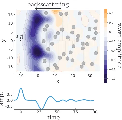
Figure 1 illustrates a backscattered wave in time mea-sured at one point in space. We consider only elastic scat-tering, and scattered waves that have the same frequency as the incident wave. We show that, with this simple setup, it is possible to recover a wide range of

Artur L. Goweret al.

w

a

v

e

am

p

l

it

u

d

e

x

backscattering

Fig. 1: (Colour online) The snapshot above is of a plane-wave pulse being backscattered by the grey particles, in the region

x >0, after timet= 20 (non-dimensional). The incident pulse originated at the linex=xR, then travelled towards the

parti-cles and was then backscattered. The blue line graph shows the amplitude measured at (xR,0) over time, where around time

t= 25 the backscattered waves begin to arrive. The particles occupy 10% of the volume and around 150 particles were used for these simulations.

tions and particle radiuses, even including particles with a sub-wavelength radius. We also identify which part of the backscattered signal is sensitive to the concentration and particle radius. To achieve these goals, we use learning curves from supervised machine learning, and, in doing so, we also show how to accurately predict particle radius and concentration from backscattered waves. Supervised machine learning in similar contexts has already shown great promise [8,9]. See [9] for a summary of machine learning applications in remote sensing.

The long-term goal is to develop a device, as simple as possible and with little prior information, that can deter-mine the statistical properties of the particles for a broad range of random media. To do so will require theoretical predictions, experiments and simulations of backscattered waves. A supervised learning approach can then easily combine data from these different sources to produce an algorithm that predicts particle statistics. Here we take the first step towards this goal, by using simulated data, as it is the most accurate for a broad range of media.

The most common approach to determine particle prop-erties from backscattering, to date, is to adjust the param-eters of a mathematical model until it fits the measured backscattering [2,10]. Ideally, these two approaches could be combined to produce an accurate method valid for a large range of parameters.

Simulating near-surface backscattering. – We consider a simple setting with Dirichlet boundary conditions, that is, where the scalar wave-field w= 0 on the boundary of the particles, which for acoustics corre-sponds to zero pressure, for elasticity correcorre-sponds to zero displacement and for electromagnetism corresponds to zero electric or magnetic susceptibility, depending on the polarisation. This case is particularly challenging for many of the current theoretical approaches, as they can lead to unphysical results, even for low frequency and low concen-tration, as we demonstrate below. We restricted ourselves to two dimensions to lighten the computational load, which is qualitatively similar to three dimensions [11]. In the conclusion we discuss extensions to three dimensions. Consider an incident plane wave eik(x−xR₋t)_{, wherekis}

the wave number of the background medium, and we have non-dimensionalised by taking the phase velocity of the background to be 1. We non-dimensionalise because the theory applies to many different applications. The total wave w = eik(x−xR−t)_{+u satisfies the two-dimensional}

scalar wave equation, whereu is the backscattered wave from the particles within the half-spacex >0 and (xR,0)

is the receiver position, such as shown in fig. 1. If the receiver is close to the particles, then near-field effects will dominate and many realisations will be needed to calculate the statistical moments. To avoid this, we choose xR =

−10. We useafor particle radius,nfor number of particles

per unit area (concentration) and φ = a2_{πn for volume} fraction, and consider a wide range of media:

1%≤φ≤21%, 0.2≤a≤2.0 and 0≤k≤1, (1)

for instance, these values are typically used in emulsions, suspensions, and for atmospheric aerosols.

For random media it is convenient to use the moments ofu. That is, if Λ represents one configuration of particles, thenu=u(Λ) depends on Λ and its ensemble average is

u= u(Λ)p(Λ)dΛ, wherep(Λ) is the probability of the particles being in the configuration Λ, then the central moments are

un=(u− u)n1/n. (2)

We will now associate each medium with a fixed particle radius, concentration and set of momentsuand (2).

There are many specialised methods to determine these moments [12–16]. Those that accurately calculate uj

for a broad frequency range require u, and a com-mon approximation of u is to assume that u ≈

eik∗x inside the random media, for some effective wave

number k∗. For small volume fraction φ and direct

backscattering [17,18] this approximation leads to u ≈ −iφ(πa2_k2₎−1

nJn(ka)/Hn(ka)ei(nπ−kx),whereJn and

Hn are a Bessel and Hankel function of the first kind.

Characterising particulate media from backscattering

Fig. 2: (Colour online) The backscattering of the incident wave e−0.1(x−xR−t)2 _{from particles of radius a= 0.2 occupyingφ=} 20% of the volume. Left: backscattering from five different configurations. Right: the moments of 756 configurations. The height of the black line is u the mean response, while the total thickness of the green and red regions are the secondu2

(standard deviation) and fourthu4 (kurtosis) moment.

a result of strong scatterers, withw = 0 on their bound-aries, completely reflecting waves at low frequencies for any particle volume fraction. This can be seen by inves-tigating the effective properties [19,20]. The consequence is that series expansions ofufor small volume fractions do not converge for scatterers withw= 0 on their bound-aries. For other strong scatterers with w ≈ 0 on their boundaries, this series converges very slowly.

It may be possible to accurately describe backscattering from strong scatterers with integral methods that are valid for any volume fraction [21,22]. Though, we note, that methods derived from Lippmann–Schwinger–type equa-tions are not formally valid for scatterers with discon-tinuous material properties [23], such as strong acoustic scatterers.

To accurately determine all the moments over the range (1), we use a numerical approach based on the multipole method [24] to calculate u(Λ) for each con-figuration Λ, from which we determine the un with

a Monte Carlo method1_{. In all our convergence tests,} truncation errors and benchmarks were within 1% accu-racy for each simulation. In the supplementary material Supplementarymaterial.pdf(SM) we explain how to re-produce our results, including high-performance software to simulate the backscattering [26] and implement the ma-chine learning. The data used in this paper is also publicly available [27].

Approximating the backscattering from an infinite halfspace, with a limited computational domain, is chal-lenging. To overcome this challenge we calculate the backscattering of the incident time pulse e−0.1(x−xR−t)2_,

which, for wave numbers 0≤ k ≤1, results in less than 1% Gibbs phenomena, and receive the backscattering at (xR,0). By only receiving the signal for t ≤ 98, we can

exclude from the simulation all particles that would take more thant= 100 for their first scattered wave to arrive at the receiver (xR,0). That is, we need only simulate

par-ticles that are near the surface, which is why we call this

near-surface backscattering. See fig. 2 for the incident time

1_{The alternative would be to piece together different theoretical}

methods, whose range of validity is not clear [25].

Fig. 3: (Colour online) An overview of the moments of the direct backscattering of the incident wave shown in the top right. Each graph shows−1< y <0.35, while thex-axis shows time 9.5≤t≤98. Each column has the same volume fraction

φ, while each row has the same particle radiusa, except in the top right which is shown to the same scale as the moments, but with time−9.5≤t≤78 and−0.35< y <1.0.

pulse and foru,u1 andu4, where we includeu4as it is known to be sensitive the micro-structure [16,28].

In total we simulated the moments of 205 different media, evenly sampled from (1), which required 83000 backscattering simulations —each corresponding to one configuration Λ. For the larger simulations up to 7600 particles were used. To estimate the quality of the calcu-lated moments, we used the standard error of the mean. See fig. 3 for an overview of the simulated moments.

Learning from backscattering. – With a high-quality data set of backscattered waves, we can now use supervised machine learning to generate amodel

that best fits the radius and a separate model that best fits the concentration. To test these models, we use them to predict the concentration and the radius of yet unseen media using only backscattered waves as input. Our supervised machine learning method of choice is kernel ridge regression [29,30], because when using continuous kernels it can fit any continuous function [31]. This allows us to establish whether the radius or the concentration are continuous functions ofu or u2 or both. In other words, we can determine which moments are needed to predict the radius and concentration. We present the results for concentration, instead of volume fraction, because it can be accurately predicted from justu.

Ourtrainingset consists of the simulated backscattered moments of 205 different media. Using this training set we

traina model, that is to say, we use kernel ridge regression applied to the training set to generate a model. The hy-perparameters of the ridge regression were selected using a 7-fold cross-validation. To determine thepredictive power

of our model, we generate atest setwith 81 randomly cho-sen media with radius 0.2 ≤a≤2.0 and volume fraction 1%≤φ≤21%. Every medium of the test set is distinct

Artur L. Goweret al.

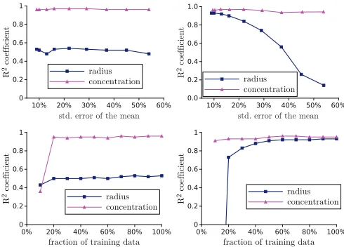
Fig. 4: (Colour online) This figure shows that to accurately predict concentration requires onlyu, but to accurately pre-dict the particle radius requires also second momentu2. The

top two models were trained using only the mean u, while the bottom two were trained using the mean u and second momentu2. The best prediction for the concentration gives

R2 = 0.98, which results from using low wave numbers, dis-cussed later.

from the training set. To measure the goodness of fit, we use theR2_{coefficient with respect to the mean of the test} set. If R2 _{= 0, then the model has the same predictive} power as the mean of the test set, while R2 _{= 1 shows} that the model has perfect prediction. Finally we tested two continuous kernels, the Gaussian (or radial basis) and the Ornstein-Uhlenbeck kernel. Both kernels gave simi-lar scores through cross-validation, though the Ornstein-Uhlenbeck kernel had a slightly better R2 _{coefficient on} the test set, so we only report these results.

Results. – We train two models using onlyu, one to predict the concentration and one to predict the radius, see the top graphs of fig. 4. The top left and top right graphs show the scatter plot of the concentration and ra-dius of the test set against the predicted concentration and radius, respectively. The prediction for the concen-tration is almost perfect, with R2 _{= 0.96. On the other} hand, the prediction for the radius is almost meaningless withR2_{= 0.53.The failure of the first moment ualone} to predict the radius is significant, as it indicates that the radius is not a continuous function ofu.

To accurately predict the radius, the second moment was necessary. Indeed, training a model on the first and second moment resulted in an accurate prediction of the radius withR2= 0.93, see the bottom right panel of fig. 4. To show that our results, such as the top right panel of fig. 4, are not due to insufficient data, and likely ex-tend beyond our data set, we examine the learning curves. A learning curve shows theR2 _{coefficient as the quality} of the data is increased. For example, if it was possi-ble to predict the radius from onlyu, then the model’s R2_{coefficient would increase when improving the training} data’s quality. Contrary to this, if theR2_{coefficient does}

Fig. 5: (Colour online) This figure shows how increasing the maximum wave number does not lead to better predictions of particle radius when measuringu. That is, for each point (x, y) on the graphs, we limit the incident wave numbers of the training and test set to 0≤k ≤x, which results in y=R2. On the left (right) we used a model trained on only u (u andu2).

Fig. 6: (Colour online) This figure shows how well the particle radius and concentration are predicted,R2, when changing the quality of the training data. The test set was fixed with a relative standard error of the mean of 10%. The top two graphs increase the number of simulations per medium, resulting in a change of the relative standard error of meanuon thex-axis. The bottom graphs increase the number of media, shown as a percentage of the full training data on thex-axis. The model on the left (right) was trained using onlyu(uandu2).

not increase, or if there is no clear trend, then the model cannot predict the radius, no matter the quality of the training data.

Characterising particulate media from backscattering

converges to R2 _{= 1. In contrast, the concentration is} accurately predicted fromueven when using either 30% of the number of training media, having large standard errors of the mean, or using only wave numbersk ≤0.1. In fact limiting 0≤k≤0.1 leads to anR2= 0.98 for the concentration.

Finally, from fig. 5, we see that the learning curve sat-urates around a maximum wave number of 0.8. This in-dicates that 0 < k < 0.8 is the ideal range to measure particles in the range 0< a <2.

Conclusions. – Our results indicate that the first di-rect backscattered momentudoes not carry information about a broad range of particle radiuses, for strong scatter-ers. However, the second momentu2does carry this in-formation. On the other hand, the particle concentration can be accurately predicted from justu. We also demon-strated that only incident wave numbers 0 < k < 0.8 are needed to accurately measure particles with radius 0 < a < 2. This implies that neither theory, simula-tion or experiments need go beyondka= 1.6, at least for strong scatterers. This also means that we are able to ac-curately recover radiuses that are 20 times smaller than the smallest incident wavelength.

In this study we did not consider limitations in spatial and temporal resolution, which, of course, are important in practice. However, before specialising to one particular scenario,i.e., typical acoustics and light scattering exper-iments, we need to know what is possible to measure or not in an ideal setting. Studies like these are therefore a vital first step. Another important step is to quantify how uncertainties in the measurements affect the prediction of the particle properties. This can be achieved by using Guassian process regression [32], which is, in a sense, a Bayesian version of kernel ridge regression.

Ultimately, our machine learning model could be em-bedded into a device to predict particulate properties. Though our model is initially trained on simulated data, our training procedure is simple enough that the model can be updated using real data. This step of adapt-ing models trained on simulated data to real applications has been applied to challenging problems such as robotic grasping [33], facial recognition [34], 3D pose inference [35] and optical flow estimation [36] to name a few. These applications have advanced in strides by using simulated data, and we see a similar potential for characterising ran-dom media, such as this work.

Both the simulation (near-surface backscattering) and machine learning approach we have presented could be ap-plied to characterise any type of particulate material from wave backscattering. To extend our approach, to 3D and other types of particles, computational efficiency is im-portant. Simulating the backscattered moments would be faster if the multilevel Monte Carlo methods [37] and fast multipole methods [38] were used. For instance, it may be possible to measure the physical properties of the parti-cles, as well as the size and concentration. Another avenue

to create more backscattering data is to piece together dif-ferent theoretical models, which could then be validated with the numeric approach we introduced: near-surface backscattering in time.

∗ ∗ ∗

ALG, WJP and IDA are grateful for the funding provided by EPSRC (EP/M026205/1, EP/L018039/1). RMG is grateful for funding provided by the FSMP at the INRIA - SIERRA project-team. JD would like to ac-knowledge the receipt of an EPSRC CASE studentship from the School of Mathematics and Thales UK.

REFERENCES

[1] Challis R. E., Povey M. J. W., Mather M. L. and

Holmes A. K.,Rep. Prog. Phys.,68(2005) 1541. [2] Thorne P. D. and Hurther D., Cont. Shelf Res., 73

(2014) 97.

[3] Hu P. and Turner J. A., J. Acoust. Soc. Am., 137 (2015) 321.

[4] Winebrenner D. P., Tsang L., Wen B.andWest R., IEEE J. Ocean. Eng.,14(1989) 149.

[5] Torres O., Bhartia P. K., Herman J. R., Ahmad Z.

and Gleason J.,J. Geophys. Res.: Atmos.,103(1998) 17099.

[6] Almasian M., Leeuwen T. G. and Faber D. J.,Sci. Rep.,7(2017) 14873.

[7] Yi J., Radosevich A. J., Rogers J. D., Norris S. C. P., Apolu l. R., Taflove A.andBackman V., Opt. Express,21(2013) 9043.

[8] Rupp M., Tkatchenko A., Mller K.-R. and von

Lilienfeld O. A.,Phys. Rev. Lett.,108(2012) 058301. [9] Noia A. D. and Hasekamp O. P., Neural Networks

and Support Vector Machines and Their Application to Aerosol and Cloud Remote Sensing: A Review, in Springer Series in Light Scattering (Springer, Cham) 2018, pp. 279–329.

[10] Weser R., Wckel S., Wessely B. and Hempel U., Ultrasonics,53(2013) 706.

[11] Galaz B., Haat G., Berti R., Taulier N., Amman J.-J.and Urbach W.,J. Acoust. Soc. Am.,127(2010) 148.

[12] Martin P. A., J. Acoust. Soc. Am., 129 (2011) 1685.

[13] Mishchenko M. I., Travis L. D.andLacis A. A., Mul-tiple Scattering of Light by Particles: Radiative Trans-fer and Coherent Backscattering (Cambridge University Press) 2006.

[14] Snieder R.,Phys. Rev. E,66_{(2002) 046615.}

[15] Garnier J. and Slna K., Arch. Ration. Mech. Anal., 220_{(2016) 37.}

[16] Sheng P.,Introduction to Wave Scattering, Localization and Mesoscopic Phenomena, inSpringer Ser. Mater. Sci., Vol.88(Springer Science & Business Media) 2006. [17] Foldy L. L.,Phys. Rev.,67(1945) 107.

[18] Gower A. L., Smith M. J., Parnell W. J.and Abra-hams I. D.,Proc. R. Soc. A,474(2018) 20170864. [19] Parnell W. J. and Abrahams I. D., Waves Random

Complex Media,20(2010) 678.

Artur L. Goweret al.

[20] Martin P. A., Maurel A. and Parnell W. J.,

J. Acoust. Soc. Am.,128(2010) 571.

[21] Cobus L. A., Tiggelen B. A. v., Derode A.andPage J. H.,Eur. Phys. J. ST,226(2017) 1549.

[22] Kristensson G.,J. Quant. Spectrosc. Radiat. Transfer, 164(2015) 97.

[23] Martin P.,SIAM J. Appl. Math.,64(2003) 297. [24] Martin P. A.,Multiple Scattering: Interaction of

Time-Harmonic Waves with N Obstacles, in Encyclopedia of Mathematics and its Applications Series, Vol.107 (Cam-bridge University Press) 2006.

[25] Tourin A., Fink M.andDerode A.,Waves in Random Medias,10(2000) R31.

[26] Gower A. L.andDeakin J., jondea/multiplescattering. jl: Version 0.1 (December 2017).

[27] Gower A. L.andDeakin J.,Backscattering from ran-domly placed Dirichlet particles (version 1.0.0).

[28] Ammari H., Garnier J., Jing W., Kang H., Lim M., Slna K. andWang H.,Mathematical and Statisti-cal Methods for Multistatic Imaging, Lect. Notes Math., Vol. 2098 (Springer International Publishing, Cham) 2013.

[29] Boser B. E., Guyon I. M.andVapnik V. N.,A training algorithm for optimal margin classifiers, inProceedings of the Fifth Annual Workshop on Computational Learning Theory COLT ’92 (ACM, New York, NY, USA) 1992, pp. 144–152.

[30] Aizerman M. A., Braverman E. A.andRozonoer L., Theoretical foundations of the potential function method in pattern recognition learning, inProceedings of Automa-tion and Remote Control, no. 25 (1964) pp. 821–837. [31] Micchelli C. A., Xu Y.andZhang H.,J. Mach. Learn.

Res.,6(2006) 2651.

[32] Rasmussen C. E. andWilliams C. K.,Gaussian Pro-cess for Machine Learning(MIT Press) 2006.

[33] Peng Xue Bin, Andrychowicz Marcin, Waremba

Wojciech and Abbeel Pieter, arXiv:1710.06537 [cs.RO] (2018).

[34] Zhao J., Xiong L., Karlekar Jayashree P., Li J., Zhao F., Wang Z., Sugiri Pranata P., Sheng-mei Shen P., Yan S.andFeng J.,Dual-agent gans for photorealistic and identity preserving profile face synthe-sis, in Advances in Neural Information Processing Sys-tems 30, edited byGuyon I., Luxburg U. V., Bengio S., Wallach H., Fergus R., Vishwanathan S. and

Garnett R.(Curran Associates, Inc.) 2017, pp. 66–76. [35] Rad M., Oberweger M.and Lepetit V., arXiv:1712.

03904 [cs.CV] (2018).

[36] Mayer N., Ilg E., Fischer P., Hazirbas C., Cremers D., Dosovitskiy A. and Brox T., to be published in Int. J. Comput. Vis.(2018),https://doi.org/10.1007/ s11263-018-1082-6.

[37] Giles M. B.,Acta Numer.,24_{(2015) 259.}