This is a repository copy of Carbon concentration declines with decay class in tropical forest woody debris.
White Rose Research Online URL for this paper: http://eprints.whiterose.ac.uk/113330/
Version: Accepted Version
Article:
Chao, K-J, Chen, Y-S, Song, G-ZM et al. (4 more authors) (2017) Carbon concentration declines with decay class in tropical forest woody debris. Forest Ecology and
Management, 391. pp. 75-85. ISSN 0378-1127 https://doi.org/10.1016/j.foreco.2017.01.020
© 2017 Elsevier B.V. This manuscript version is made available under the CC-BY-NC-ND 4.0 license http://creativecommons.org/licenses/by-nc-nd/4.0/
eprints@whiterose.ac.uk
Reuse
Unless indicated otherwise, fulltext items are protected by copyright with all rights reserved. The copyright exception in section 29 of the Copyright, Designs and Patents Act 1988 allows the making of a single copy solely for the purpose of non-commercial research or private study within the limits of fair dealing. The publisher or other rights-holder may allow further reproduction and re-use of this version - refer to the White Rose Research Online record for this item. Where records identify the publisher as the copyright holder, users can verify any specific terms of use on the publisher’s website.
Takedown
If you consider content in White Rose Research Online to be in breach of UK law, please notify us by
Carbon concentration declines with decay class in tropical forest woody debris 1
2
Kuo-Jung Chaoa*, Yi-Sheng Chenb, Guo-Zhang Michael Songc, Yuan-Mou Changd, 3
Chiou-Rong Sheueb, Oliver L. Phillipse & Chang-Fu Hsiehf 4
5
aInternational Master Program of Agriculture, National Chung Hsing University,
6
Taichung 40227, Taiwan 7
bDepartment of Life Sciences, National Chung Hsing University, Taichung 40227,
8
Taiwan 9
cDepartment of Soil and Water Conservation, National Chung Hsing University,
10
Taichung 40227, Taiwan 11
dDepartment of Ecoscience and Ecotechnology, National University of Tainan, Tainan
12
70005, Taiwan 13
eSchool of Geography, University of Leeds, Leeds, LS2 9JT, UK
14
fInstitute of Ecology and Evolutionary Biology, National Taiwan University, Taipei
15
10617, Taiwan 16
* Corresponding author. 17
E-mail address: kjungchao@dragon.nchu.edu.tw (Kuo-Jung Chao).
Abstract
19Carbon stored in woody debris is a key carbon pool in forest ecosystems. The most 20
widely-used method to convert woody debris volume to carbon is by first multiplying 21
field-measured volume with wood density to obtain necromass, and then assuming that 22
a fixed proportion (often 50%) of the necromass is carbon. However, this crucial 23
assumption is rarely tested directly, especially in the tropics. The aim of this study is to 24
verify the field carbon concentration values of living trees and woody debris in two 25
distinct tropical forests in Taiwan. Wood from living trees and woody debris across all 26
five decay classes was sampled to measure density and carbon concentrations. We 27
found that both wood density and carbon concentration (carbon mass / total mass) 28
declined significantly with the decay class of the wood. Mean ( SE) carbon 29
concentration values for living trees were 44.6 ± 0.1%, while for decay classes one to 30
five they were respectively 41.1 ± 1.4%, 41.4 ± 1.0%, 37.7 ± 1.3%, 30.5 ± 2.0%, and 31
19.6 ± 2.2%. Total necromass carbon stock was low, only 3.33 0.55 Mg C ha-1 in the
32
windward forest (Lanjenchi) and 4.65 1.63 Mg C ha-1 in the lowland forest 33
(Nanjenshan). Applying the conventional 50% necromass carbon fraction value would 34
cause a substantial overestimate of the carbon stocks in woody debris of between 17% 35
and 36%, or about 1 Mg of carbon per hectare. The decline in carbon concentration and 36
the increase of variances in the heavily decayed class suggest that in high-diversity 37
tropical forests there are diverse decomposition trajectories and that assuming a fixed 38
carbon fraction across woody pieces is not justified. Our work reveals the need to 39
consider site-specific and decay class-specific carbon concentrations in order to 40
accurately estimate carbon stocks and fluxes in forest ecosystems. If the marked decline 41
44
Keywords: Carbon content, Decomposition, Necromass, Woody debris, Specific 45
gravity, Tropical forest 46
47
1
Introduction
48
Natural forest ecosystems may help mitigate the increasing atmospheric carbon 49
concentration caused by human activities (Malhi et al., 1999). Therefore, many studies 50
have tried to estimate the carbon stocks and fluxes in forest ecosystems to evaluate their 51
dynamics and carbon balance (e.g., Brienen et al., 2015; Rice et al., 2004; Saner et al., 52
2012; Wilcke et al., 2005). The major carbon pools in forest ecosystems include 53
biomass (living trees), necromass (woody debris), and soil organic matter (Saner et al., 54
2012). Although necromass accounts for a smaller proportion (6% to 25%) of the 55
vegetative mass pools than biomass, neglecting the carbon store and fluxes associated 56
with woody debris can lead to inaccuracies and greater uncertainty when attempting to 57
estimate the whole carbon balance in forest ecosystems (Chao et al., 2009; Nascimento 58
and Laurance, 2002; Rice et al., 2004). 59
60
Many woody debris studies inventoried volumes and mass of woody debris, but not 61
carbon concentration (Russell et al., 2015). Carbon concentration (also known as 62
carbon fraction or carbon content; the proportion of carbon per unit dry mass) is in fact 63
a rarely studied variable both for living trees (Martin and Thomas, 2011; Thomas and 64
Martin, 2012) and woody debris (Russell et al., 2015). When no field data are available, 65
the conventional approach is assuming that a fixed value, often 50%, of dry mass is 66
carbon for living trees (e.g. Brienen et al., 2015; Houghton, 2005), woody debris (e.g. 67
al., 2013; Rice et al., 2004). 69
70
Some field-based studies have shown that carbon concentration can vary significantly 71
for living trees (Elias and Potvin, 2003). For example, a recent review showed that 72
carbon concentration of living trees can range from 41.9 to 51.6% in tropical species, 73
45.7 to 60.7% in subtropical and Mediterranean, and 43.4 to 55.6% in temperate and 74
boreal species (Thomas and Martin, 2012). The Intergovernmental Panel on Climate 75
Change (IPCC) also recommended that when forest-type-specific carbon concentration 76
are not available, the value 47% as carbon should be used for tropical rainforests, in 77
order to estimate national carbon storage and carbon emissions (IPCC, 2006). Therefore, 78
the use of 50% as carbon concentration may be inappropriate, and may introduce errors 79
of more than 10% into tropical forest biomass carbon estimates (Elias and Potvin, 2003). 80
Thus, precise and large-scale estimates of forest carbon content cannot be achieved 81
without fine-scaled and forest-type-specific carbon concentration values (IPCC, 2006). 82
83
The carbon concentration of woody debris also needs to be inventoried (Harmon et al., 84
2013; Russell et al., 2015; Weggler et al., 2012). There is yet no consensus about the 85
relationships between carbon concentration and decay classes of woody debris for at 86
least two reasons. First, decay classes of woody debris vary study-to-study. Classes are 87
subjectively defined by researchers in the field, generally based on morphological traits 88
and hardness of samples (Harmon et al., 1986; Russell et al., 2015). The commonly 89
used number of decay class is a five-class system, but it can range from two to eight 90
classes, depending on the researcher interest (Harmon et al., 1986; Russell et al., 2015). 91
The general rule is that the less the structural integrity of woody debris, the higher the 92
carbon concentration among decay classes in woody debris, their results are 94
inconsistent, and have variable sample size. For example, in temperate and boreal forest 95
studies, some found that the concentration barely changes with decay classes (Mäkinen 96
et al., 2006; Weggler et al., 2012). However, one study did find that carbon 97
concentration per unit dry mass can be low for the highly decomposed samples 98
(Carmona et al., 2002). In contrast, another found a significant increase in carbon 99
concentration for gymnosperms with increasing decay class (Harmon et al., 2013). 100
Based on our review, only four studies have attempted to examine the carbon 101
concentration of woody debris in tropical forests (Clark et al., 2002; Iwashita et al., 102
2013; Meriem et al., 2016; Wilcke et al., 2005). These suggest either similar carbon 103
concentrations among decay classes, ranging from 40.0 to 47.9% (Iwashita et al., 2013; 104
Meriem et al., 2016; Wilcke et al., 2005), or slight declines with decay class (Clark et 105
al., 2002). The sample sizes of these tropical studies ranged from 16 (Wilcke et al., 106
2005) to 261 (Meriem et al., 2016) per study plot. As necromass is one of the important 107
carbon pools in tropical forests (Chao et al., 2009), and one which may potentially be 108
increasing as mortality rates increase with drought frequency (Brienen et al., 2015), it 109
is critical to quantify and understand variations in carbon concentration both for living 110
trees and woody debris in tropical forests. 111
112
Here, we investigate the wood density and carbon concentration values of woody debris 113
among decay classes in tropical forests in Taiwan, as a contribution to improve the 114
accuracy of carbon stocks and flux estimation in tropical forest ecosystems. Total 115
necromass of two distinct forest types was measured in order to estimate the carbon 116
stocks in these forests. We aimed to uncover patterns of carbon concentration change 117
concentration among living trees and woody debris within the same forests. We also 119
aimed to sample at sufficient intensity to make robust conclusions about the direction 120
of relationship, if any, between carbon fraction and woody decay. Other elements, e.g. 121
nitrogen and hydrogen, were also measured in order to have an overview of chemical 122
components in our samples. 123
124
2
Methods
125
2.1 Study sites
126
The study sites are located in the Nanjenshan Reserve, Kenting National Park, Taiwan. 127
The mean temperature is 22.7 °C and mean annual rainfall ranges from 3252 mm in the 128
lowland forests to 3989 mm on windward mountain summit in the reserve (Chao et al., 129
2010b). Soils are classified as Typic Paleudults, characterised by highly weathering 130
pedogenesis and relatively low cation concentration in the slopes facing the northeast 131
monsoon wind (Chen et al., 1997). Several Forest Dynamics Plots were established 132
since 1989 in order to monitor the ecology of the forest ecosystems in this reserve (Chao 133
et al., 2007; Chao et al., 2010b). We collected samples of living trees and woody debris 134
in two forest types: one is a tropical lowland windswept evergreen dwarf forest 135
(Lanjenchi Plot; 5.88 ha), and the other is a tropical lowland evergreen broad-leaved 136
forests (Nanjenshan Plot I and Nanjenshan Plot II; 2.1 ha and 0.64 ha, respectively) 137
(Chao et al., 2010b). The definition of forest types followed Taiwan Forestry Bureau 138
(2011). Lanjenchi Plot suffers from wind of northeast monsoon in winters and its 139
dominant species are Illicium arborescens, Castanopsis cuspidate var. carlesii, and 140
Schefflera octophylla (Chao et al., 2010b). The forest canopy height varied from 3 m at 141
the windward summit to 15 m in valley (Chao et al., 2010b). Both Nanjenshan Plots I 142
Plot, and their dominant species are Ficus benjamina, Psychotria rubra, and Dysoxylum 144
hongkongense (Chao et al., 2010b). The forest canopy height is 15 to 20 m (Chao et al., 145
2010b). Samples collected from Nanjenshan Plots I and II were treated from the same 146
forest as the plots were floristically and structurally similar to each other (Chao et al., 147
2010a; Chao et al., 2010b). Therefore, hereafter we denote the samples collected in 148
Nanjenshan Plots I and II simply as Nanjenshan Plots. Typhoons in summer are the 149
dominant disturbance type for both forests. For detailed vegetation composition please 150
refer to Chao et al. (2010b). 151
152
2.2 Wood sample collection and property measurements
153
Wood cores of living trees were taken in January to February 2015 for wood density 154
and carbon concentration measurements. Ten out of the top 15 dominant tree species of 155
the Lanjenchi Plot (Chao et al., 2007) and of the Nanjenshan Plots (Chao et al., 2010a) 156
were selected (Appendix 1). The ranks of species dominance were based on their basal 157
area within each forest (as listed in Chao et al., 2010a; Chao et al., 2007). For each selected 158
species, one to three living individuals were chosen for wood coring. For each sampled 159
individual, one core was taken by an increment borer (number of sampled wood cores 160
n = 30 in the Lanjenchi Plot; n = 27 in the Nanjenshan Plots; Appendix 1). The 161
individuals were randomly selected from outside the study plots (within 500 m) in order 162
to prevent damage to the tagged living individuals within the Forest Dynamics Plots. 163
We only sampled individuals with DBH (diameter at 1.3 m height) ≥ 7 cm, in order to
164
reduce the risk of mortality caused by wood core sampling. We assumed that these 165
samples from dominant species represent plot-level averages of living trees. 166
Woody debris is defined here as all dead, woody material of trees with diameter larger 168
than 1 cm. We walked along the four border lines of each plot, and collected woody 169
debris samples outside the plots for wood density measurement. These samples were 170
collected in July 2012 outside the Lanjenchi Plot (woody debris, n = 378) and inJuly
171
2009 outside the Nanjenshan Plots I and II (woody debris, n = 357). Carbon 172
concentration samples were collected in February 2013 within the plots (Lanjenchi Plot, 173
n = 95 and the Nanjenshan Plots, n = 95), avoiding those woody debris crossed by the 174
volume transect lines. As it is very difficult to identify the species of woody debris in 175
species-rich tropical forests, we intended to collect a plot-level representative sample 176
pool. This meant that samples were collected throughout the plots to represent dominant 177
species and microhabitats in our plots. 178
179
We used the five decay class system to classify the woody debris samples, based on 180
morphology and hardness observed in the field (modified from Harmon et al., 1986) 181
(Table 1). Living trees were designated as having decay class 0 in our study. To evaluate 182
whether necromass decay class classification depended subjectively on individual 183
investigators or not, we performed a simple analysis by comparing decay class 184
classification among two main investigators (YSC and CML) with 455 woody debris 185
samples, each scored independently. We found that 83.3% of the samples were 186
classified in the same decay class. For 6.8% of samples YSC scored 1 decay class lower 187
than CML, for 9.7% of samples that YSC scored 1 decay class higher than CML, and 188
for 0.2% of the samples (one sample) YSC scored 2 decay classes higher than CML. 189
The findings suggested that there is some small between-researcher variation in the 190
subjective classification (uncertainty), but that there was no systematic difference either 191
determining the decay class (Larjavaara and Muller-Landau, 2010) is not suitable for 193
our study sites since the majority of woody debris pieces in the field are smaller than 194
196
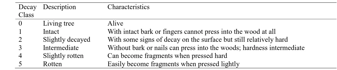
Table 1. Description of woody debris decay classes (modified from Harmon et al., 1986). 197
Decay Class
Description Characteristics
0 Living tree Alive
1 Intact With intact bark or fingers cannot press into the wood at all
2 Slightly decayed With some signs of decay on the surface but still relatively hard
3 Intermediate Without bark or nails can press into the woods; hardness intermediate
4 Slightly rotten Can become fragments when pressed hard
5 Rotten Easily become fragments when pressed lightly
199
The majority of samples (living trees and woody debris) were taken back to the 200
laboratory, in the form of wood cores, wood disks or chunks. For wood density (dry 201
weight/volume) measurements, fresh volumes were measured by the water 202
displacement method (Chave et al., 2006). Some samples in the decay class five (59 203
out of 73 samples) were too fragile to be measured by the water displacement method. 204
These samples were collected in the field by a fixed-volume cup (volume = 33.07 ml). 205
The fixed-volume cup can assist wood density measurement and avoid seriously fresh 206
volume compaction when taking those samples back to the laboratory. All samples for 207
wood density measurement were oven dried (65 ºC for living woods and 70 ºC for 208
woody debris) until the weight of samples was relatively constant. Wood density ( ; g 209
cm-3) was calculated as the ratio of oven-dry weight (g) to fresh volume (cm3) (total n
210
= 792, including living trees (n = 57) and woody debris (n = 735)). 211
212
For woody debris carbon concentration measurements, samples were collected in the 213
field in the form of woody disks or chunks. As there is no need to take fixed volume 214
samples for carbon concentration measurement, fragile samples were collected and 215
placed into envelopes. Although Harmon et al. (2013) have demonstrated that bark 216
could have higher carbon concentration than heartwood and sapwood in temperate and 217
boreal forests, we did not separate our woody debris samples into tissue types. This is 218
because bark can-not be reliably distinguished from other tissues types in heavily 219
decayed samples in our sites. All collected samples were oven-dried at 65 ºC for one 220
week. Once the weight was constant, a cross section of each sample was sawed to 221
collect a set of well mixed sawdust, representing its proportion of tissue types. Each set 222
trees were similarly ground from bark to heartwood. The equipment (saw, mortar, and 224
pestle) was cleaned with a gas gun to prevent any between sample contamination. For 225
each sample, the finely ground powders were collected and well-mixed. A fine 226
subsample of these powders (1.3 to 3.9 mg) was put into a tin capsule for weight 227
measurement. For each piece of wood two powder samples were used to derive each 228
piece’s average carbon concentration and nitrogen concentration values. Acetanilid 229
(71.09% carbon (C), 10.36% nitrogen (N), and 6.71% hydrogen (H)) was used as a 230
standard for analysing the C, N and H elements in the samples. Total sample size of 231
element concentration analyses (C, N and H) was 247, including 57 living trees and 190 232
woody debris. The measurements were conducted using Elemental analyzers in 233
National University of Tainan (2400 Series II CHNS/O Analyzer, Perkin Elmer, 234
California, USA; n = 43) and in National Chung Hsing University (vario EL III 235
CHNS/O Analyzer, Elementar Analysensysteme GmbH, Hanau, Germany; n = 204). 236
237
Six samples at the decay class five (three samples from the Lanjenchi Plot and three 238
from the Nanjenshan Plots) were subjectively selected based on their carbon 239
concentrations for further chemical element analysis in oxygen (O), sulphur (S) and 240
wood ash percentages. The vario EL III CHNS/O Analyzer in National Chung Hsing 241
University (Elementar Analysensysteme GmbH, Hanau, Germany) was used for the 242
oxygen and sulphur analyses. The standard for analysing the oxygen is Benzoic acid 243
(26.20% oxygen), and for analysing the sulphur is Sulfanilic acid (18.50% sulphur). 244
Wood ash percentage was determined in an ashing furnace (Carbolite CWF 13/5 245
Laboratory Chamber Furnace, 5 Liters, Carbolite, UK) by heating to 550 to 600 °C for 246
24 h. After the weights of samples have become relatively constant, the remaining ash 247
249
In the literature, the temperature required to dry the carbon concentration samples 250
ranges from freeze-drying conditions (Martin and Thomas, 2011), 55 ºC (Harmon et al., 251
2013), 65 ºC (Weggler et al., 2012), 80 ºC (Clark et al., 2002), and 110 ºC (Martin and 252
Thomas, 2011). We chose to use 65 ºC as a trade-off between the loss of both water and 253
of volatile carbon at high temperatures. This is because wood dried at 105 ºC can 254
increase about 0.8% to 1% carbon content (due to additional dehydration) (Weggler et 255
al., 2012) but can also cause loss of volatile carbon (about 2.48%) (Martin and Thomas, 256
2011). 257
258
2.3 Necromass estimation
259
Necromass is estimated as the product of volume and wood density. We measured the 260
volumes of two types of above-ground woody debris (fallen and standing) in the 261
Lanjenchi and Nanjenshan plots annually since 2012. Necromass in the Lanjenchi Plot 262
has been inventoried four times (2012, 2013, 2014, and 2015), and in the Nanjenshan 263
Plots three times (2013, 2014, and 2015). We used the line-intersect method for 264
quantifying fallen woody debris (van Wagner, 1968) and the plot-based method for 265
standing woody debris, such that standing woody debris on either side (5 m) of the line-266
intersect transects (i.e. 10 m width in total) were recorded. Fallen woody debris was 267
defined as those fragmented woody branches or trunks either lying on the ground or 268
stuck above-ground level. All fallen woody debris with intercepted diameter ≥ 1 cm 269
was measured, and its diameter, void proportion, decay class and locality were recorded. 270
Standing woody debris was defined as those dead trunks still upright and rooted to the 271
soil. Void proportion is defined as the proportion of hollow space observable from the 272
as standing woody debris. All standing woody debris with diameter ≥ 1 cm at base 274
(close to ground) and ≥ 0.02 m in length within the sampled quadrats was measured.
275
The measurements made included base diameter, void proportion, decay class, top 276
diameter (where ≥ 1 cm or equal to 1 cm), and height. The top diameters and height of 277
the main trunk of standing dead wood were all visually estimated, using the hands-278
raised height of researchers (ca. 2 to 2.2 m) as a scale. Any remaining fine branches on 279
top of standing woody debris were ignored, as the volume is small and visual estimates 280
of this fraction would lack accuracy; we focused on the main trunk of standing woody 281
debris and it is therefore likely we very slightly underestimated total woody debris 282
volume. 283
284
Five transects were established in Lanjenchi, five in Nanjenshan Plot I, and three in 285
Nanjenshan Plot II. These were oriented a priori along two perpendicular directions, 286
east to west and north to south, in order to reduce the possibility of systematic bias 287
affecting the necromass estimates (Bell et al., 1996). In the Lanjenchi Plot, three of the 288
transects were oriented from east to west, with total lengths of 198, 200, and 280 m, 289
respectively, and two oriented from north to south with total lengths of 194 and 198 m. 290
In Nanjenshan Plot I, two transects were oriented east to west with total lengths of 100 291
and 105 m, and three from north to south with total lengths of 105, 105 and 111 m. In 292
Nanjenshan Plot II, one transect was oriented from east to west, with total length of 60 293
m, and two from north to south with total lengths of 60 and 64 m. 294
295
Volumes of fallen woody debris were estimated using the method proposed by van 296
Wagner (1968): 297
where V is the volume at unit area (m3 ha-1), d is the intercepted diameter (cm) for each 299
fallen woody debris, and L in the total length (m) of each transect. If void proportion 300
was recorded in the field, the d 2 of each sample was further multiplied by (100 % − 301
void proportion (%)) to exclude void space. The averages of the plot-level volumes of 302
fallen woody debris were weighted by transect length. 303
304
Volumes of standing woody debris were estimated using the Smalian’s formula (Phillip, 305
1994): 306
v = ( /8) ×LS ×(db2+dt2), eqn 2
307
where v is the volume (m3) of the target standing woody debris, db and dt (m) are the
308
diameters at base and top, respectively, and LS (m) is the length of the target standing
309
woody debris. If void proportion was recorded in the field, v was further multiplied by 310
(100 % − void proportion (%)). The averages of the plot-level volumes of standing 311
woody debris were weighted by transect length. 312
313
Plot-level variance ( 2) values were also weighted by transect length as suggested by 314
(Keller et al., 2004). 315
= Ln-1j Vij-Lj2, eqn 3 316
where Lj is the length of each transect; Vij is the measured volume of each transect j (m3
317
ha-1) at the decay class i; is the weighted average of each plot at the decay class i; n 318
is the number of sampled transects. Standard error of the mean (SE) was calculated as 319
/ . Plot-level SE is the sum of each SE at each decay class. 320
321
Necromass of each decay class is calculated by Mi = i × Vi, where Mi is necromass at
322
decay class i, i is average wood density at decay class i and Vi is volume at decay class
i. Carbon stock of each decay class is calculated by CSi = ci × Mi, where CSi is carbon
324
stock at decay class i, ci is carbon concentration at decay class i and Mi is necromass at
325
decay class i. 326
327
The standard error of M i is
328
SEM i = SE i × V i + SEVi × i, eqn 4
329
where SEi and SEVi are the standard errors in density and volume at decay class i,
330
respectively (Keller et al., 2004). The same function was applied for the standard error 331
of carbon concentration. 332
333
2.4 Statistical analysis 334
Weighted and unweighted linear regressions were used to find the relationships between 335
dependent and independent variables. When a dependent variable y (e.g. wood density, 336
carbon concentration, or nitrogen concentration) had homogeneous variances ( 2) for
337
different values of an independent variable x (e.g. decay class), then unweighted linear 338
regressions were applied. We tested whether residuals varied with the fitted values of 339
independent variables (Appendix 2), indicating that y did not have homogeneous 2
340
with decay class, and in these cases a weighted regression was used (James et al., 2013). 341
The weights for each independent variable value, x, were the inverse of an estimated 342
variance function ( , where is the estimated variance function (Appendix
343
3). Weighted and unweighted linear regressions were performed with the lm() function 344
in the program R, version 3.3.0 (R Core Team, 2016). Other statistical analyses were 345
carried out by IBM SPSS Statistics v. 20 (IBM Corporation, New York, USA). 346
3
Results
3483.1 Wood density and carbon concentration of living trees
349
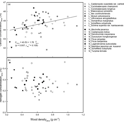
For living trees, carbon concentration (% carbon per unit mass; Calive) had a significant
350
relationship with the wood density (g cm-3) of living trees ( alive) (Fig. 1a), whereas
351
nitrogen concentration (%) did not (Fig. 1b). The results showed that for living trees, 352
species with high wood density are likely to also have high carbon concentration (Fig. 353
1a). 354
355
3.2 Wood properties among decay classes
356
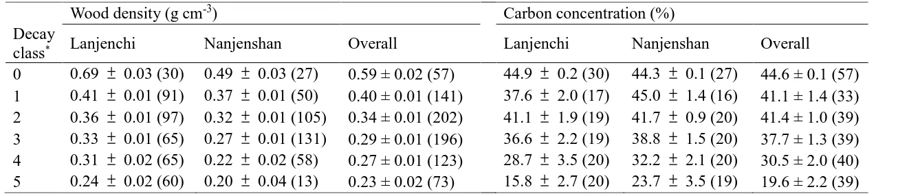
Wood density and carbon concentration of living trees and woody debris decreased with 357
decay class in the study plots (Table 2), whereas nitrogen concentration has an 358
increasing trend (Table 3). There was a significant difference between plots in wood 359
density values and nitrogen concentration, such that wood in the Lanjenchi Plot had 360
higher wood density and lower nitrogen concentration than in the Nanjenshan Plots 361
(Mann-Whitney U tests, both p values < 0.001; Table 2; Table 3). However, there was 362
no significant difference between plots in carbon concentration values (Mann-Whitney 363
U test, p = 0.627) (Table 2). 364
365
As preliminary tests found that neither dependent variable had constant variance 366
(Appendix 2), weighted regressions were used to find the best-fitted mean functions 367
and variance functions (Fig. 2). Notably, the mean function of carbon concentration 368
declined with decay classes. Moreover, the conventional value 50% was significantly 369
higher than carbon concentration of both living and woody debris samples (one sample 370
nitrogen concentration all increased with decay classes, indicating that the higher the 372
decay classes, the higher the variability (Fig. 2). 373
374
Nitrogen concentration (%) in both plots increased slightly with decay classes (Table 3; 375
Fig. 2c). In contrast, the patterns of C:N ratio decreased significantly from living trees 376
to heavily decayed woody debris (decay class 5) (two-way ANOVA, ln transformed 377
C:N ratio, decay class F[5, 247] = 14.264, p = 0.006; plot F[1, 247] = 9.345, p = 0.028; Table
378
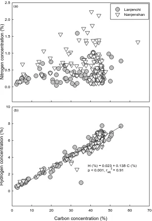
3). There is no significant relationship between carbon concentration and nitrogen 379
concentration (Fig 3a), but the relationship between carbon concentration and hydrogen 380
concentration is significantly positive for all the living trees and woody debris samples 381
(Fig. 3b). 382
383
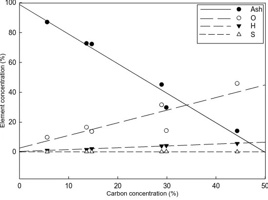
To better understand the chemical properties of decayed wood, we further examined the 384
proportion of oxygen, hydrogen, sulphur, and ash of six pieces in the decay class five 385
(Fig. 4). The six pieces were subsampled from the decay class five pool (three samples 386
from the Lanjenchi Plot and three samples from Nanjenshan Plots). The samples were 387
subjectively selected in order to represent a wide range of carbon concentration (ranging 388
from 5.63% to 44.33%). Examining the six samples, we found a significant negative 389
relationship between ash (%) and carbon (%), suggesting an accumulation of inorganic 390
elements with the decay of carbon. Ash concentration can reach values as high as 87%. 391
Fig. 1 Relationships between wood density and other elements of living trees. 393
(a) Carbon concentration of living trees (Calive; %) has significant relationship with
394
wood density ( alive; g cm-3) of the same individual (unweighted regression; p = 0.007,
395
radj2 = 0.108, n = 57). (b) Relationship between wood density and nitrogen concentration
396
(Nalive; %) of living trees is not significant (unweighted regression; p = 0.242, n = 57).
397
L_: samples from the Lanjenchi Plot; N_: samples from the Nanjenshan Plots. Detailed 398
species information please refer to Appendix 1. 399
Wood densityalive (g cm-3)
0.2 0.4 0.6 0.8 1.0 1.2
0.0 0.1 0.2 0.3 0.4 0.5 Nitrog en concen tratio
naliv
e (% ) Car bo n concen tratio
naliv
e (% ) 41 42 43 44 45 46 47 N_Bischofia javanica N_Castanopsis indica N_Dendrocnide meyeniana N_Dysoxylum hongkongense N_Ficus ampelas N_Ficus benjamina N_Lagerstroemia subcostata N_Machilus japonica var. kusanoi N_Schefflera octophylla N_Turpinia ternata
L_Castanopsis cuspidata var. carlesii L_Cyclobalanopsis championii L_Cyclobalanopsis longinux L_Elaeocarpus sylvestris L_Ilex cochinchinensis L_Illicium arborescens L_Lithocarpus amygdalifolius L_Osmanthus marginatus L_Schefflera octophylla
L_Schima superba var. kankaoensis
Calive = 43.53 + 1.76 alive
(p = 0.007, radj 2
= 0.108) (a)
400
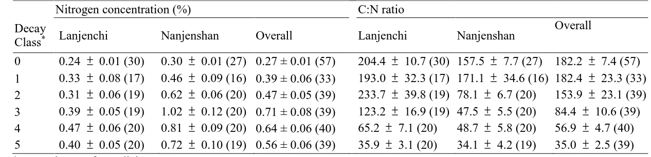
Table 2. Wood density and carbon concentration of living trees and woody debris in Lanjenchi and Nanjenshan Forest Dynamics Plots, Taiwan. 401
(mean SE (n); n = sample size) 402
Wood density (g cm-3) Carbon concentration (%)
Decay
class* Lanjenchi Nanjenshan Overall Lanjenchi Nanjenshan Overall
0 0.69 0.03 (30) 0.49 0.03 (27) 0.59 ± 0.02 (57) 44.9 0.2 (30) 44.3 0.1 (27) 44.6 ± 0.1 (57)
1 0.41 0.01 (91) 0.37 0.01 (50) 0.40 ± 0.01 (141) 37.6 2.0 (17) 45.0 1.4 (16) 41.1 ± 1.4 (33)
2 0.36 0.01 (97) 0.32 0.01 (105) 0.34 ± 0.01 (202) 41.1 1.9 (19) 41.7 0.9 (20) 41.4 ± 1.0 (39)
3 0.33 0.01 (65) 0.27 0.01 (131) 0.29 ± 0.01 (196) 36.6 2.2 (19) 38.8 1.5 (20) 37.7 ± 1.3 (39)
4 0.31 0.02 (65) 0.22 0.02 (58) 0.27 ± 0.01 (123) 28.7 3.5 (20) 32.2 2.1 (20) 30.5 ± 2.0 (40)
5 0.24 0.02 (60) 0.20 0.04 (13) 0.23 ± 0.02 (73) 15.8 2.7 (20) 23.7 3.5 (19) 19.6 ± 2.2 (39)
*Decay class 0 refers to living trees
W ood dens it y (g c m -3 ) 0.0 0.2 0.4 0.6 0.8 1.0 1.2 Lanjenchi Nanjenshan mean mean + SD mean - SD = 0.51 - 0.11 x + 0.01 x2 + 0.07 x0.5
(p < 0.001, radj2 = 0.25)
C arbon c onc ent ration (% ) 0 10 20 30 40 50 60 70
C = 44.55 - 0.94 x2 + 6.08 x0.5 (p < 0.001, radj2 = 0.46)
C = 50
Decay class
0 1 2 3 4 5
N it rog en c onc ent ration (% ) 0.0 0.5 1.0 1.5 2.0 2.5
N = 0.26 + 0.17 x - 0.02 x2 + 0.25 x0.5 (p < 0.001, radj2 = 0.24)
(a)
(b)
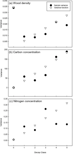
Fig. 2 (a) Wood density, (b) carbon concentration, and (c) nitrogen concentration among 405
decay classes in the Lanjenchi and Nanjenshan Forest Dynamics Plots, Taiwan. 406
Solid lines are weighted regressions (mean functions) for all the samples and dash-407
dotted lines were the mean functions ± standard deviation ( x ) functions. The 408
dotted line in (b) is the reference line for C = 50. The mean function ± standard deviation 409
function at each figures are (a) = 0.51 - 0.11 x + 0.01 x2 ± 0.07 x0.5 (weighted regression; 410
p < 0.001, radj2 = 0.25, n = 792; is wood density (g cm-3) and x is the decay class). (b)
411
C = 44.55 – 0.94 x2 ± 6.08 x0.5 (weighted regression; p < 0.001, radj2 = 0.46, n = 247; C
412
is carbon concentration (%)). (c) N = 0.26 + 0.17 x - 0.02 x2 ± 0.25 x0.5 (weighted 413
regression; p < 0.001, radj2 = 0.24, n = 247; N is nitrogen concentration (%)). Decay
414
416
Table 3. Nitrogen concentration (%) and C:N ratio of living trees and woody debris in Lanjenchi and Nanjenshan Forest Dynamics Plots, Taiwan. 417
(mean SE (n); n = sample size) 418
Nitrogen concentration (%) C:N ratio
Decay
Class* Lanjenchi Nanjenshan Overall Lanjenchi Nanjenshan
Overall
0 0.24 0.01 (30) 0.30 0.01 (27) 0.27 ± 0.01 (57) 204.4 10.7 (30) 157.5 7.7 (27) 182.2 7.4 (57)
1 0.33 0.08 (17) 0.46 0.09 (16) 0.39 ± 0.06 (33) 193.0 32.3 (17) 171.1 34.6 (16) 182.4 23.3 (33)
2 0.31 0.06 (19) 0.62 0.06 (20) 0.47 ± 0.05 (39) 233.7 39.8 (19) 78.1 6.7 (20) 153.9 23.1 (39)
3 0.39 0.05 (19) 1.02 0.12 (20) 0.71 ± 0.08 (39) 123.2 16.9 (19) 47.5 5.5 (20) 84.4 10.6 (39)
4 0.47 0.06 (20) 0.81 0.09 (20) 0.64 ± 0.06 (40) 65.2 7.1 (20) 48.7 5.8 (20) 56.9 4.7 (40)
5 0.40 0.05 (20) 0.72 0.10 (19) 0.56 ± 0.06 (39) 35.9 3.1 (20) 34.1 4.2 (19) 35.0 2.5 (39)
*Decay class 0 refers to living trees
Fig. 3 Relationships between carbon concentration and other elements. 420
Both living trees and woody debris were included in the figures. (a) No significant 421
relationship between carbon concentration (C; %) and nitrogen concentration (N; %) 422
(unweighted regression, p = 0.105, n = 247). (b) The relationship between carbon 423
concentration and hydrogen concentration (H; %) was significant (unweighted 424
regression, H = 0.023 + 0.138 C, p < 0.001, radj2 = 0.91, n = 204).
425
426
Nitr
og
en
c
oncent
rat
ion
(%)
0.0 0.5 1.0 1.5 2.0 2.5
Lanjenchi Nanjenshan
Carbon concentration (%)
0 10 20 30 40 50 60 70
Hy
dr
og
en
c
oncent
rat
ion
(%)
0 2 4 6 8 10
H (%) = 0.023 + 0.138 C (%) p < 0.001, radj
2 = 0.91 (a)
427
Fig. 4 Relationships between carbon (C) and other chemical elements of woody debris 428
at decay class five. Oxygen (O), hydrogen (H), sulphur (S) and ash concentrations were 429
plotted against carbon concentration (n = 6). The lower the carbon concentration the 430
higher the ash concentration (unweighted regression, ash = 98.8 - 2.0 C, p < 0.001, radj2
431
= 0.96, n = 6), suggesting that inorganic components accumulate as woody debris 432
becomes de-carbonised. Other elements (H and O) were positively related to the carbon 433
concentration in the decay class five (unweighted regression, p <0.001 and p = 0.028), 434
but sulphur did not (p = 0.414). 435
436
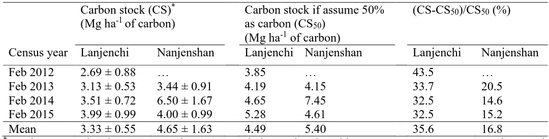
3.3 Necromass and carbon stocks
437
The total above-ground necromass was 8.99 ± 1.24 Mg ha-1 (mean ± SE) in Lanjenchi
438
and 10.81 ± 3.58 Mg ha-1 in Nanjenshan (Table 4). The Lanjenchi plot in general had
439
more fine necromass (32.3% of total necromass) then the Nanjenshan plots (20.6% of 440
total necromass) (Table 4). Average ratios of standing to fallen woody debris varied 441
between 0.26 and 0.68 (Table 4). Applying our measured carbon concentration (%) to 442
necromass at each decay class, we estimated a woody debris carbon stock of 3.33 ± 443
Carbon concentration (%)
0 10 20 30 40 50
El
em
en
t c
on
ce
n
tra
ti
on
(%
)
0 20 40 60 80 100
0.55 Mg ha-1 in Lanjenchi and 4.65 ± 1.63 Mg ha-1 in Nanjenshan plots (Table 5). If we 444
had simply assumed that carbon is 50% of the necromass, then the carbon stocks in the 445
forests would have been overestimated by from 16.8% to 35.6% (Table 5). 446
448
Table 4. Necromass (mean ± SE), fine necromass proportion (diameter smaller than 10 cm), and standing to fallen woody debris mass ratio (S/F) 449
in Lanjenchi and Nanjenshan Forest Dynamics Plots, Taiwan. 450
Necromass total (Mg ha-1) Fine necromass proportion (%)* S/F
Census year Lanjenchi Nanjenshan Lanjenchi Nanjenshan Lanjenchi Nanjenshan
Feb 2012 7.71 ± 1.98 … 28.6 … 0.57 …
Feb 2013 8.37 ± 1.01 8.29 ± 1.93 30.6 22.2 0.58 0.56
Feb 2014 9.30 ± 1.41 14.90 ± 3.37 34.5 16.4 0.31 0.29
Feb 2015 10.56 ± 2.09 9.23 ± 1.99 35.5 23.3 0.26 0.68
Mean 8.99 ± 1.24 10.81 ± 3.58 32.3 20.6 0.43 0.51
* proportion of mass
451
453
Table 5. Carbon stock (mean ± SE) in Lanjenchi and Nanjenshan Forest Dynamics Plots, Taiwan. 454
Carbon stock (CS)* (Mg ha-1 of carbon)
Carbon stock if assume 50% as carbon (CS50)
(Mg ha-1 of carbon)
(CS-CS50)/CS50 (%)
Census year Lanjenchi Nanjenshan Lanjenchi Nanjenshan Lanjenchi Nanjenshan
Feb 2012 2.69 ± 0.88 … 3.85 … 43.5 …
Feb 2013 3.13 ± 0.53 3.44 ± 0.91 4.19 4.15 33.7 20.5
Feb 2014 3.51 ± 0.72 6.50 ± 1.67 4.65 7.45 32.5 14.6
Feb 2015 3.99 ± 0.99 4.00 ± 0.99 5.28 4.61 32.5 15.2
Mean 3.33 ± 0.55 4.65 ± 1.63 4.49 5.40 35.6 16.8
* Apply measured carbon concentration (%) at each decay class in Table 2 to convert necromass to carbon stock
456
4
Discussion
457
There has been surprisingly little attention paid to determining the carbon concentration 458
of tropical forest woody debris, with no tropical study having simultaneously compared 459
carbon concentration among living trees and woody debris within the same plots (Table 460
6). Our study showed that in our studied tropical forests the carbon concentration of 461
necromass can decrease significantly with the decay of wood (Fig. 2). Moreover, 462
regardless of level of decay, carbon concentration is substantially below the value (50% 463
of dry mass; one sample t-test, p < 0.001) that has been applied as an approximation of 464
carbon concentration for carbon stored in biomass (Houghton et al., 2001; Rice et al., 465
2004) and woody debris (Chao et al., 2009; Ngo et al., 2013). This demonstrates that a 466
finer scale and forest-type-specific carbon concentration values may be needed for 467
accurate estimate of necromass carbon stock, and by extension total ecosystem carbon 468
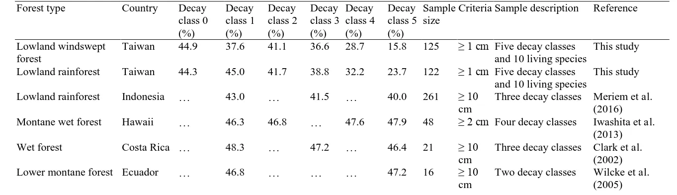
470
Table 6 Carbon concentration (%) of woody debris in tropical forestry literature. 471
Forest type Country Decay
class 0 (%)
Decay class 1 (%)
Decay class 2 (%)
Decay class 3 (%)
Decay class 4 (%)
Decay class 5 (%)
Sample size
Criteria Sample description Reference
Lowland windswept forest
Taiwan 44.9 37.6 41.1 36.6 28.7 15.8 125 ≥ 1 cm Five decay classes
and 10 living species
This study
Lowland rainforest Taiwan 44.3 45.0 41.7 38.8 32.2 23.7 122 ≥ 1 cm Five decay classes
and 10 living species
This study
Lowland rainforest Indonesia … 43.0 … 41.5 … 40.0 261 ≥ 10
cm
Three decay classes Meriem et al. (2016)
Montane wet forest Hawaii … 46.3 46.8 … 47.6 47.9 48 ≥ 2 cm Four decay classes Iwashita et al.
(2013)
Wet forest Costa Rica … 48.3 … 47.2 … 46.4 21 ≥ 10
cm
Three decay classes Clark et al. (2002)
Lower montane forest Ecuador … 46.8 … … … 47.2 16 ≥ 10
cm
Two decay classes Wilcke et al.
(2005)
473
4.1 Wood density and carbon concentration of living trees
474
Carbon concentration of living trees in tropical forests ranges from 41.9 to 51.6% 475
(Thomas and Martin, 2012). In our studied forests, the carbon concentrations of living 476
trees are relatively low (Appendix 1). Nonetheless, our results do support the suggestion 477
in Elias and Potvin (2003) that the proportion of carbon of living trees is related to the 478
wood density (Fig. 1a). For those forests lacking any measurement of carbon 479
concentration, it is therefore possible to apply species wood density to estimate the 480
carbon concentration of living trees. This will be an attractive practical choice for many 481
researchers because the measurement of wood density is a much easier and cheaper 482
undertaking than the measurement of carbon concentration (Elias and Potvin, 2003). 483
Moreover, applying the available global wood density databases (e.g. Zanne et al., 2009) 484
can help to better estimate carbon concentration of tropical trees. 485
486
Our recommendations for carbon concentration estimation of living trees are as follows. 487
At a lowest-level of certainty (e.g. IPCC Tier 1), researchers can apply a fixed value of 488
carbon concentration from a similar ecosystem (e.g. Table 4.3 in IPCC, 2006). At an 489
intermediate-level of certainty, researchers can apply equations developed from a 490
similar ecosystem to convert wood density to carbon concentration (such as Fig. 1a for 491
Southeast Asian tropical forests). At a more specific level, researchers should apply 492
species-specific carbon concentration values based on in situ field measurements. 493
494
4.2 Wood density and carbon concentration among decay classes
495
Converting volume to carbon requires knowing both wood density and carbon 496
that both wood density and carbon concentration decline significantly with the class of 498
decay (Fig. 2). The decline of wood density with decay classes is a common finding 499
among studies and ecosystems (e.g.: Chao et al., 2008; Clark et al., 2002; Mackensen 500
and Bauhus, 2003). It underlines the importance of measuring the density of woody 501
debris to help achieve greater accuracy in estimates of necromass. Simply assuming 502
woody debris has the same wood density as living trees would result in overestimating 503
the necromass (Weggler et al., 2012). 504
505
As for the carbon concentration, many studies have for convenience used a fixed value 506
(e.g. 50%) of mass as carbon in both biomass and necromass (Brienen et al., 2015; 507
Chao et al., 2009; Coomes et al., 2002; Latte et al., 2013). We found that carbon 508
concentration decreased markedly with decay classes (Table 2; Fig. 2). Our findings 509
contradict with previous studies which found that carbon concentration seems relatively 510
constant among decay classes in tropical forests (Iwashita et al., 2013; Meriem et al., 511
2016; Wilcke et al., 2005) (Table 6). Only a single study from Costa Rica (Clark et al., 512
2002) suggested that the carbon concentration by mass might slightly decrease with 513
advancing decay class. By contrast, a direct measurement of woody debris 514
decomposition (which is not based on decay classes) in tropical China found that there 515
was a significant decrease of carbon concentration after 9 years of observation (Yang et 516
al., 2010). The apparent divergence between these studies merits further investigation, 517
especially because it suggests that the underlying mechanisms involved may differ. 518
519
Besides the patterns of mean values, our study also found that the variances of carbon 520
increased with decay class (Fig. 2b). This is a common pattern among tropical, 521
al., 2016). This suggests that element concentration can vary greatly for heavily 523
decayed pieces which is due to the complicated decomposition trajectories. Thus, it is 524
important to acquire adequate sample sizes to achieve reliable conclusions. As 525
decomposition trajectory involves the interactions between woody substrates, 526
decomposer organisms, and climatic characteristics (Berbeco et al., 2012; Harmon et 527
al., 1986; Weedon et al., 2009; Yang et al., 2010), we hypothesise that a fixed carbon 528
fraction (i.e. steady carbon release) across woody pieces may not be typical for high-529
biodiversity tropical forests. 530
531
Several mechanisms may contribute to the high variation of carbon content of woody 532
pieces among and within decay classes. For substrate characteristics, we suspect that 533
the chemical properties of wood and tissue type proportions are crucial factors. 534
Decomposition can be simplified into two major processes: fragmentation (physical and 535
biological fragmentation) and mineralisation (leaching and respiration) (Harmon et al., 536
1986). The decrease of carbon concentration for any piece of wood is likely due to 537
leaching of soluble carbohydrates and respiration of labile carbon compounds (Fujisaki 538
and Perrin, 2015). For example, soluble carbohydrates would decrease with the increase 539
of lignin concentration during decomposition, as lignin is relatively recalcitrant 540
(Ganjegunte et al., 2004). Therefore, the original proportion of these carbohydrate 541
compounds of wood pieces may influence the carbon concentration in woody debris 542
with decay classes, and result in the high variability in carbon concentration among 543
heavily decayed pieces (Fig. 2b). 544
545
Differences in tissue type proportions among wood may also contribute to the variation. 546
bark samples can have slightly greater (about 1.0%) carbon concentrations than the 548
interior woody parts. Although we did not separate the tissue types, field observation 549
showed that majority of the woody debris at decay class four and five were lacking bark, 550
or their bark barely distinguishable from other tissue types. This can be due to in tropical 551
rainforests where fire or temperature seasonality is not an issue for plant survival, trees 552
usually have thinner outer barks (Rosell, 2016). In contrast, some woody pieces at decay 553
class four and five in our study plots only have outer bark and hollow interiors. Thus, 554
the high variances in carbon concentration in heavily decayed wood are likely due to 555
divergent decomposition trajectories, including potentially differing susceptibility of 556
bark. The overall decline in carbon concentration with decay class in our forests may 557
also be, to some extent, associated with the lack of bark tissue in the more decayed 558
woody debris pieces. 559
560
Other mechanisms related to decomposer organisms and climatic characteristics also 561
are worth further investigation. For example, Schilling et al. (2015) have demonstrated 562
that the decomposer community (e.g. fungi) has significant influence on the declining 563
patterns of woody debris properties, especially on lignin and wood density. Microsite 564
moisture and temperature also can significantly influence wood decomposition (e.g. 565
Berbeco et al., 2012; Jomura et al., 2015), although the effects on carbon concentration 566
are not clear yet. Thus, further studies should focus on comparing the variation in 567
substrate quality (chemical properties and tissue types), decomposer communities, and 568
climatic characteristics across regions and forest types. These variations may be 569
responsible for the large variance and the potential declining or increasing patterns of 570
carbon concentration in decayed woods. 571
4.3 Woody debris characters between forests 573
Species composition has been suggested to be an issue in affecting elemental 574
concentrations of necromass, at least in some temperate and boreal forests (Harmon et 575
al., 2013). Ideally, if species-specific measurements on woody debris are available, it 576
can help to disentangle the varied patterns between studies. However, in species-rich 577
tropical forests identifying woody debris at the species level is always difficult, and 578
often impossible. For this reason we used a plot-level carbon concentration for woody 579
debris. For living trees, species identification is relatively easy. Thus, we selected 580
dominant species in the plots and assumed that these represent the plot-level values in 581
living woods. Overall, the challenges with producing taxa-based woody debris carbon 582
concentrations estimates for tropical forests limit exploration of the potential role of 583
community floristic composition in explaining between-site differences in tropical 584
necromass decay. 585
586
Forest structure could be another factor affecting carbon concentration values between 587
forests, especially the diameter size of fragments. Chambers et al. (2000) showed that 588
diameter of trees is negatively related to decomposition rate. Heilmann-Clausen and 589
Christensen (2004) argue that diameter size (i.e. surface area per volume) can influence 590
decomposer community which in turn results in the divergence of decayed wood 591
property (Schilling et al., 2015). We also observed that small pieces of wood had more 592
similar outer and inner decomposition status than those of large woods. In our study 593
forests, trees are generally small in diameter due to the influences of northeast monsoon 594
wind (Chao et al., 2010b). Thus, our small forests may have faster decomposition rate, 595
differed decomposer community, and more consistent outer and inner decayed woody 596
contrary, for forests dominated by large woody pieces, a rotten woody debris piece may 598
include some less decayed (and high carbon concentration) interior. 599
600
The subjective classification of decay class, and the underlying assumption that the 601
appearance and/or hardness of woody debris represents the decomposition processes 602
can introduce uncertainty in chemical properties between studies. We suspect that the 603
application of the subjective classification may differ among forest types, especially for 604
large and heavily decayed pieces, which could potentially complicate the determination 605
of carbon concentration. Thus, there is a need to verify the actual physical (e.g. wood 606
density) and chemical (e.g. carbon concentration) indications of the decay class 607
classification scheme between forests. 608
609
4.4 Concentration of other elements among decay classes
610
What remains behind the marked decline of carbon concentration in decayed woods? 611
In general, dry mass of living wood is composed of 50% carbon, 6% hydrogen, 44% 612
oxygen, and other trace amounts of inorganics (Rowell, 2012). A minor proportion, 0.2 613
to 3.4%, is ash (Fengel and Wegener, 1989). Examining the six subsamples from decay 614
class five, we found a significant increase of ash (%) with the decrease of carbon (%), 615
but other elements, in general, increased with carbon (%) (Fig. 4). Fengel and Wegener 616
(1989) suggest that the main components of ash are inorganic components, such as 617
potassium, calcium, magnesium, and silicon. Therefore, our finding of increasing ash 618
contents in heavily decayed wood demonstrates that inorganic components tend to 619
accumulate as carbon declines over time. This is likely due to cumulative impact of 620
leaching and heterotrophic respiration of organics during wood decay (Foudyl-Bey et 621
623
The average nitrogen concentration values in wood of living trees in our study plots 624
(0.24% to 0.30%; Table 3) are similar to those from other tropical trees (average 0.24%; 625
Martin et al., 2014). Therefore, any differences in mineralisation rates appear unlikely 626
due to the differences in the nitrogen concentration in our study plots. We also found 627
that nitrogen concentration increased with decay classes, supporting the accumulation 628
of nitrogen during decomposition of woods found in other temperate (Harmon et al., 629
1986), subtropical (Ricker et al., 2016), and tropical (Clark et al., 2002; Wilcke et al., 630
2005) studies. The consistency between studies further emphasises the N retention role 631
of wood debris among sites. This accumulation of nitrogen is due to nitrogen fixation 632
and inhabitation of wood by other heterotrophs which can translocate nitrogen to the 633
decaying wood (Foudyl-Bey et al., 2016; Harmon et al., 1986). 634
635
The increase of nitrogen and decrease of carbon with the decay classes of wood resulted 636
in declining patterns of C:N ratio in our study sites (Table 3). The declining pattern is 637
also consistent with other tropical and subtropical studies (Clark et al., 2002; Meriem 638
et al., 2016; Wilcke et al., 2005; Yang et al., 2010). However, ratios were relatively low 639
in our sites (47.5 to 204.4), compared with other studies (32.4 to 365) (Clark et al., 640
2002; Fujisaki and Perrin, 2015; Meriem et al., 2016; Wilcke et al., 2005; Yang et al., 641
2010). The low C:N ratio of wood indicates potential for high respiration rate and fast 642
decay (Mackensen and Bauhus, 2003). 643
644
Oxygen and hydrogen percentages are highly correlated with carbon concentration (Fig. 645
3 and Fig. 4), suggesting that they are parts of the carbohydrate components. Thus, their 646
decay classes. Other compounds and elements which did not measured in our study, 648
such as P and Mg (Wilcke et al., 2005) and decay-resistant phenol-based extractives 649
(Harmon et al., 2013), may also accumulate with decomposition. These suggest that 650
woody debris can accumulate nutrients in the process of decomposition while losing 651
mass and carbon. In our forests at least, although the overall quantity of necromass is 652
generally low in the fully decayed class, such heavily decayed woody debris is rich in 653
inorganic nutrients. 654
655
4.5 Conclusions
656
The “carbon conversion factor” (wood density × carbon concentration) has been 657
suggested by the IPCC (2006) as a required parameter to be able to estimate forest 658
carbon stocks and emissions. As the classification of decay class is subjective and 659
simply based on the appearance of wood pieces (e.g. Table 1), there is a need to verify 660
the actual physical (e.g. wood density) and chemical (e.g. carbon concentration) 661
indications of the decay class classification scheme. Our study reveals a pattern of 662
decreasing carbon concentration with decay status of wood within tropical forests in 663
Taiwan and also a pattern of increasing variance in the heavily decayed class. We 664
hypothesise that a fixed carbon fraction (i.e. steady carbon release) across woody pieces 665
is unlikely to be typical for high-biodiversity tropical forests due to diverse 666
decomposition trajectories involving variable woody substrate quality, decomposer 667
organism activities, and climatic conditions. Applying the conventional 50% carbon 668
concentration would substantially overestimate the carbon stores in woody debris, 669
potentially by more than a third. We therefore identify here a clear need to move beyond 670
applying blanket assumptions about carbon concentration in necromass, and instead to 671
our study plots are rather small, if the marked decline in carbon fraction with necromass 673
decay turns out to be a widespread phenomenon across tropical forests, then the size of 674
the dead wood carbon pool in the biome is likely to be somewhat less than simple mass-675
based calculations would suggest. 676
677
5
Acknowledgements
678
We sincerely appreciate the great assistance in fieldwork from Yen-Chen Chao, Chia-679
Min Lin, Hui-Ru Lin, Chia-Wen Chen, Chien-Hui Liao and numerous volunteers. We 680
also thank Dr. Peter Chesson for the critical statistical help and Dr. Sheng-Yang Wang 681
for comments and supports on the chemical analyses. This study was funded by grants 682
to Kuo-Jung Chao from the Ministry of Science and Technology, Taiwan (NSC 101 - 683
2313 - B - 005 - 024 - MY3 and MOST 104 - 2313 - B - 005 - 032 - MY3). Oliver L. 684
Phillips is supported by an ERC Advanced Grant (T-Forces) and is a Royal Society-685
Wolfson Research Merit Award holder. 686
687
6
References
688
Ashton, P.S., Hall, P., 1992. Comparisons of structure among mixed dipterocarp 689
forests of north-western Borneo. J. Ecol. 80, 459-481. 690
Bell, G., Kerr, A., McNickle, D., Woollons, R., 1996. Accuracy of the line 691
intersect method of post-logging sampling under orientation bias. For. Ecol. Manage. 692
84, 23-28. 693
Berbeco, M.R., Melillo, J.M., Orians, C.M., 2012. Soil warming accelerates 694
decomposition of fine woody debris. Plant Soil. 356, 405-417. 695
Brienen, R.J.W., Phillips, O.L., Feldpausch, T.R., Gloor, E., Baker, T.R., Lloyd, 696
Martinez, R., Alexiades, M., Álvarez Dávila, E., Alvarez-Loayza, P., Andrade, A., 698
Aragão, L.E.O.C., Araujo-Murakami, A., Arets, E.J.M.M., Arroyo, L., C., G.A.A., 699
Bánki, O.S., Baraloto, C., Barroso, J., Bonal, D., Boot, R.G.A., Camargo, J.L.C., 700
Castilho, C.V., Chama, V., Chao, K.J., Chave, J., Comiskey, J.A., Cornejo Valverde, F., 701
da Costa, L., de Oliveira, E.A., Di Fiore, A., Erwin, T.L., Fauset, S., Forsthofer, M., 702
Galbraith, D.R., Grahame, E.S., Groot, N., Hérault, B., Higuchi, N., Honorio Coronado, 703
E.N., Keeling, H., Killeen, T.J., Laurance, W.F., Laurance, S., Licona, J., Magnussen, 704
W.E., Marimon, B.S., Marimon-Junior, B.H., Mendoza, C., Neill, D.A., Nogueira, E.M., 705
Núñez, P., Pallqui Camacho, N.C., Parada, A., Pardo-Molina, G., Peacock, J., Peña-706
Claros, M., Pickavance, G.C., Pitman, N.C.A., Poorter, L., Prieto, A., Quesada, C.A., 707
Ramírez, F., Ramírez-Angulo, H., Restrepo, Z., Roopsind, A., Rudas, A., Salomão, R.P., 708
Schwarz, M., Silva, N., Silva-Espejo, J.E., Silveira, M., Stropp, J., Talbot, J., ter Steege, 709
H., Teran-Aguilar, J., Terborgh, J., Thomas-Caesar, R., Toledo, M., Torello-Raventos, 710
M., Umetsu, R.K., van der Heijden, G.M.F., van der Hout, P., Guimarães Vieira, I.C., 711
Vieira, S.A., Vilanova, E., Vos, V.A., Zagt, R.J., 2015. Long-term decline of the 712
Amazon carbon sink. Nature. 519, 344-348. 713
Carmona, M.R., Armesto, J.J., Aravena, J.C., Pérez, C.A., 2002. Coarse woody 714
debris biomass in successional and primary temperate forests in Chiloé Island, Chile. 715
For. Ecol. Manage. 164, 265-275. 716
Chambers, J.Q., Higuchi, N., Schimel, J.P., Ferreira, L.V., Melack, J.M., 2000. 717
Decomposition and carbon cycling of dead trees in tropical forests of the central 718
Amazon. Oecologia. 122, 380-388. 719
Chao, K.-J., Chao, W.-C., Chen, K.-M., Hsieh, C.-F., 2010a. Vegetation dynamics 720
of a lowland rainforest at the northern border of the Paleotropics at Nanjenshan, 721
Chao, K.-J., Phillips, O.L., Baker, T.R., 2008. Wood density and stocks of coarse 723
woody debris in a northwestern Amazonian landscape. Can. J. For. Res. 38, 795-825. 724
Chao, K.-J., Phillips, O.L., Baker, T.R., Peacock, J., Lopez-Gonzalez, G., 725
Martínez, R.V., Monteagudo, A., Torres-Lezama, A., 2009. After trees die: quantities 726
and determinants of necromass across Amazonia. Biogeosciences. 6, 1615-1626. 727
Chao, W.-C., Chao, K.-J., Song, G.-Z.M., Hsieh, C.-F., 2007. Species 728
composition and structure of the lowland subtropical rainforest at Lanjenchi, southern 729
Taiwan. Taiwania. 52, 253-269. 730
Chao, W.-C., Song, G.-Z., Chao, K.-J., Liao, C.-C., Fan, S.-W., Wu, S.-H., Hsieh, 731
T.-H., Sun, I.-F., Kuo, Y.-L., Hsieh, C.-F., 2010b. Lowland rainforests in southern 732
Taiwan and Lanyu, at the northern border of paleotropics and under the influence of 733
monsoon wind. Plant Ecol. 210, 1-17. 734
Chave, J., Muller-Landau, H.C., Baker, T.R., Easdale, T.A., ter Steege, H., Webb, 735
C.O., 2006. Regional and phylogenetic variation of wood density across 2456 736
neotropical tree species. Ecol. Appl. 16, 2356-2367. 737
Chen, Z.-S., Hsieh, C.-F., Jiang, F.-Y., Hsieh, T.-H., Sun, I.-F., 1997. Relations of 738
soil properties to topography and vegetation in a subtropical rain forest in southern 739
Taiwan. Plant Ecol. 132, 229-241. 740
Clark, D.B., Clark, D.A., Brown, S., Oberbauer, S.F., Veldkamp, E., 2002. Stocks 741
and flows of coarse woody debris across a tropical rain forest nutrient and topography 742
gradient. For. Ecol. Manage. 164, 237-248. 743
Coomes, D.A., Allen, R.B., Scott, N.A., Goulding, C., Beets, P., 2002. Designing 744
systems to monitor carbon stocks in forests and shrublands. For. Ecol. Manage. 164, 745
89-108. 746
carbon concentration for 32 neotropical tree species. Can. J. For. Res. 33, 1039-1045. 748
Feldpausch, T.R., Rondon, M.A., Fernandes, E.C.M., Riha, S.J., Wandelli, E., 749
2004. Carbon and nutrient accumulation in secondary forests regenerating on pastures 750
in central Amazonia. Ecol. Appl. 14, 164–176. 751
Fengel, D., Wegener, G., 1989. Wood---Chemistry, Ultrastructure, Reactions, 752
Walter de Gruyter, Berlin. 753
Foudyl-Bey, S., Brais, S., Drouin, P., 2016. Litter heterogeneity modulates fungal 754
activity, C mineralization and N retention in the boreal forest floor. Soil Biol. Biochem. 755
100, 264-275. 756
Fujisaki, K., Perrin, A.P., A. -S.)[ 1 ] ; Boussafir, M (Boussafir, M.)[ 3 ] ; Gogo, 757
S (Gogo, S.)[ 3 ] ; Sarrazin, M (Sarrazin, M.)[ 4 ] ; Brossard, M 2015. Decomposition 758
kinetics and organic geochemistry of woody debris in a ferralsol in a humid tropical 759
climate. Eur. J. Soil Sci. 66, 876-885. 760
Ganjegunte, G.K., Condron, L.M., Clinton, P.W., Davis, M.R., Mahieu, N., 2004. 761
Decomposition and nutrient release from radiata pine (Pinus radiata) coarse woody 762
debris. For. Ecol. Manage. 187, 197-211. 763
Harmon, M.E., Fasth, B., Woodall, C.W., Sexton, J., 2013. Carbon concentration 764
of standing and downed woody detritus: effects of tree taxa, decay class, position, and 765
tissue type. For. Ecol. Manage. 291, 259-267. 766
Harmon, M.E., Franklin, J.F., Swanson, F.J., Sollins, P., Gregory, S.V., Lattin, J.D., 767
Anderson, N.H., Cline, S.P., Aumen, N.G., Sedell, J.R., Lienkaemper, G.W., Cromack, 768
K.J., Cummins, K.W., 1986. Ecology of coarse woody debris in temperate ecosystems. 769
Adv. Ecol. Res. 15, 133-302. 770
Heilmann-Clausen, J., Christensen, M., 2004. Does size matter? On the 771