Performance evaluation of a model thermocompressor using computational fluid dynamics



Abstract— Thermocompressors are widely used in a large number of industries that use steam as their heating medium or as a power generating utility. They are devices that use the energy of a high pressure fluid to move a low pressure fluid and enable it to be compressed to a higher pressure according to the principle of energy conversion. They work like a vacuum pump but without usage of any moving part and so they can save energy. The performance of a thermocompressor highly depends on its geometry and operating conditions. This paper first describes the flow behavior within a designed model of a thermocompressor using the computational fluid dynamics code, FLUENT. Since the flow is turbulent and supersonic, CFD is an efficient tool to reveal the phenomena and mixing process at different part of the thermocompressor which are not simply obtained through an experimental work. Then its performance is analyzed by choosing different operating conditions at the boundaries and also different area ratios which is one of the significant geometrical factors to describe the thermocompressor performance. Finally, the effect of various nozzle exit plane diameters which cause different Mach numbers at the nozzle exit is investigated on the thermocompressor performance. The results indicate that these variables can affect both the entrainment ratio and critical back pressure. This device uses water vapor as the working fluid and operates at 7.5 bar motive pressure, 63°C and 80°C for suction and discharge temperatures, respectively.

Keywords—Thermocompressor, ejector, performance evaluation, entrainment ratio, converging-diverging nozzle, CFD.

I. INTRODUCTION

arge industrial plants often vent significant quantities of low-pressure steam to the atmosphere, wasting energy, water, and water-treatment chemicals. Recovery of the latent heat content of low-pressure steam reduces the boiler load, resulting in energy and fuel cost savings. Low-pressure steam’s potential uses include driving evaporation and distillation processes, producing hot water, space heating, producing vacuum, or chilling water. If the steam pressure is too low for the intended application, a steam jet thermocompressor or ejector can boost the pressure and temperature to the required level. Thermocompressors and ejectors operate on the same thermodynamic and physical principle: energy contained in high-pressure steam can be

Lecturer, Mechanical Engineering Department, Islamic Azad University, Neyriz Branch, Neyriz, Iran. (Email: [email protected])

transferred to a lower pressure vapor or gas to produce a mixed discharge stream of intermediate pressure. These devices are known for: simple construction, easy installation, low capital and installation costs, easy maintenance with no moving parts, long useful operating life. A high performance thermocompressor in an industry leads to the higher recovery of low pressure steam and save more energy. In order to design a high performance thermocompressor, a better understanding of the flow behavior such as shock interactions and mixing process inside it is necessary. It is also needed to have a good knowledge of the effects of various parameters on the thermocompressor performance. Previously, designers relied primarily on the past experience, analysis based on empirical formulations and test results to make the final design decisions. However, complex fluid flow behavior within the thermocompressor results in a flow field where comprehensive experimental data are too difficult and expensive to obtain. Keen and Neumann developed a classical one-dimensional theory based on the gas dynamic rule in order to design the ejectors [1]. This theory then was modified to consider the loss coefficients at different part of ejector by Eames et al. [2]. But, this theory was used to predict the performance only when the thermocompressor operates at its design condition (at critical back pressure). A number of researchers investigated the effect of jet ejector geometry on jet ejector performance. For example, Kroll [3] investigated the effect of convergence, divergence, length, and diameter of the throat section, nozzle position, induced fluid entrance, and motive velocity. Croft and Lilley investigated the optimum length and diameter of the throat section, nozzle position, and angle of divergence [4]. Eames [5] carried out an experimental work to assess the effect of ejector geometry on its performance such as nozzle design and nozzle exit location. El-Dessouky et al. [6] developed a simple empirical model to design and evaluate the performance of steam jet ejectors based on a large database extracted from several ejector manufacturers and a number of experimental literatures. Their model was simple and eliminated the need for iterative procedures. Recently, Because of the ability of the computational fluid dynamics and numerical simulation to explain the flow field inside the complex geometries, researchers tend to apply CFD in order to model and design the thermocompressors. The advantages of this method are that it takes less time and cost than experimental method for predicting the performance of a

Performance Evaluation of a Model

Thermocompressor using Computational Fluid

Dynamics

Kavous Ariafar

thermocompressor. It also guides designers to the directions in which a design should be modified to meet design objectives. CFD software has been proved by a number of researchers, Riffat and Everitt [7], Hoggarth [8], Riffat et al., [9], as a powerful tool for predicting flow fields inside jet ejectors. Riffat and Omer [10] and Da-Wen and Eames [11] studied the effect of nozzle position on jet ejector performance on both designs; constant pressure and constant-area. As a result, they found that it greatly affects jet ejector performance, as it determines the distance over which the motive and propelled stream are completely mixed. ESDU suggested that the nozzle should be placed between 0.5 and 1.0 throat diameters before the entrance of the throat section [12].

Rusly et al. simulated the flow through an R141b ejector. They investigated the effects of ejector geometries and validated their results with experimental data provided by other researchers [13]. Bartosiewicz et al. compared experimental pressure distribution data for an ejector, which used air as working fluid, with results of simulation using different turbulence models [14]. Later they extended their work using R142b as the working fluid [15].

In this study, the flow behavior is first investigated by showing the pressure distribution profile along the axis of a designed model thermocompressor. Then its performance is analyzed by choosing different operating conditions at the boundaries and also different area ratios which is one of significant geometrical factor. Finally the effect of various nozzle exit plane diameters which cause different Mach numbers at the nozzle exit is investigated on the thermocompressor performance. The CFD software package (FLUENT) is used for numerical simulations.

II. HOW THERMOCOMPRESSOR OPERATES

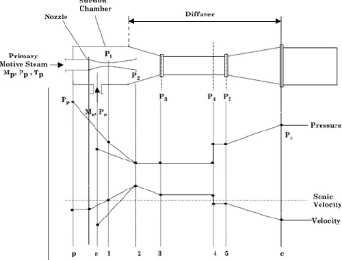
Thermocompressor essentially consists of three main parts: Nozzle, Suction Chamber and Diffuser. The nozzle and diffuser have the geometry of converging-diverging venturi or deleval nozzle. The high pressure steam that enters the nozzle is referred to as the Motive steam or Primary fluid in some literatures. The low pressure steam that is recovered is known as the Suction steam or Secondary fluid in some literatures and the steam that exits the thermocompressor from the diffuser is termed as the Discharge steam.

Figure 1 shows a schematic of the thermocompressor with pressure-velocity profile along its axis. The function of the nozzle is to convert the motive steam entering at high pressure and low velocity to a very high velocity and pressure lower than the low pressure suction steam. The velocity of steam as it enters the nozzle (at point p) increases in the converging portion. At the end of the converging portion is the throat, the smallest section of the nozzle where the velocity reaches sonic velocity. Beyond the throat, the velocity of steam increases until the tip of the nozzle (point 2) where supersonic velocities are reached and a very low pressure region is created. The steam jet leaving the nozzle meets the surrounding low pressure steam (at point e) and causes it to enter the suction chamber. The mixing process begins in the suction chamber

where provides a channel to the low pressure suction steam to reach the jet and the subsequent diffuser section. The function of the diffuser is to convert the kinetic energy to pressure energy. The mixing of the high velocity jet and the slow moving low pressure steam is completed in the converging section of the diffuser (point 3). The pressure recovery of the mixed stream begins at the later section of the converging diffuser and continues till the outlet of the thermocompressor. As the mixed stream leaves the converging part of the diffuser, it enters the smallest section of the diffuser, throat. At this stage, the fluid stream undergoes a sudden pressure rise due to occurrence of a normal shock (point 4). It leads to a sudden pressure recovery and fluid attains subsonic velocity after shock. As the fluid further moves to the diverging part of diffuser, the velocity drops further and pressure is more recovered. Finally, the fluid reaches design outlet pressure at the exit of the subsonic diffuser.

One of the important parameters to describe the performance of a thermocompressors is the Entrainment Ratio (Rm) which is defined as the ratio of the recovered Suction steam quantity to motive steam quantity. This is the ratio of mass flow rate (kg/h) of suction steam to flow rate (kg/h) of motive steam. The high entrainment ratio for a thermocompressor signifies the high quantity of steam which can be recovered and so, high performance thermocompressor has a high entrainment ratio.

Fig. 1 schematic of the thermocompressor with pressure-velocity profile along the axis

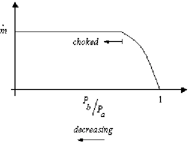
decreases, the mass flow starts to enter the nozzle and it is expected that further decreasing the back pressure causes the more mass flow rate to enter.

Fig. 2 mass flow rate through the nozzle

But it happens just up to a specific point and after that the mass flow rate stops increasing and remains constant. It doesn’t matter how much lower the back pressure is. At this point it is said that the nozzle has become choked where the flow speed at the throat reaches the speed of the sound (Mach number = 1). Each thermocompressor has the same trend for the mass flow rate according to its own operating back pressure which will be explained in the results section.

III. COMPUTATIONALMODEL A. Governing Equations

Fluid flow in the thermocompressor is typically compressible and turbulence. The governing equations to describe the compressible flow are conversation of energy, momentum and continuity which are as follows:

Continuity: D divv 0

Dt   (1)

Momentum: Dv g p _ij

Dt

      (2)

Energy: ( ) _ij i

j

Dh D v

div k T

Dt Dt x



     

 (3) The term of ij is written as:

2 ( ) 3 j i ij j i v v Idivv x x     

  (4)

The realizable k-ε turbulence model is selected to govern the turbulence characteristics in this simulation. The term “realizable” means that the model satisfies certain mathematical constraints on the Reynolds stresses, consistent with the physics of turbulent flows. An immediate benefit of the realizable k-ε model is that it more accurately predicts the spreading rate of both planar and round jets [16]. This model is a relatively recent development and differs from the standard k-ε model in two important ways:

1. The realizable k-ε model contains a new formulation for the turbulent viscosity.

2. A new transport equation for the dissipation rate, ε, has been derived from an exact equation for the transport of the mean-square vorticity fluctuation.

Basically, the k-ε turbulence model is a semi-empirical model based on model transport equations for the turbulence kinetic energy (k) and its dissipation rate (ε). The model transport equation for k is derived from the exact equation, while the model transport equation for ε is obtained using physical reasoning and is different for standard and realizable models. The numerical solution of the above mentioned set of mean equations is obtained by introducing additional transport equations for the Reynolds stresses, u ui j . These equations

introduce six variables and increase the difficulty of solving the system. Also these equations contain higher-order correlations that represent the processes of diffusion transport, viscous dissipation, and fluctuating pressure–velocity interactions. The Reynolds stresses are presumed linearly related to the mean rate of strain via a scalar eddy viscosity:

2

( )

3

j i

i j ij t

j i

U U

u u k

x x

   

  

  (5) Where k is the turbulence kinetic energy and υt is the turbulent viscosity that is calculated from:

2 ( ) t k C_  

 (6)

Where ε is the rate of dissipation of k and Cμ is one of the model constants. The local values of k and ε for realizable model are obtained from solution of their modeled transport equations

2

[( t ) ]

i t

j j k j

k k

u S

x x x



  



 _  _  _{ }

   (7)

2

1 2

[( t ) ]

j

j j j

u C S C

x x _ x  k



 _  _ 

 

 _  _  _{ }

    (8)

Where S in the modulus of the mean rate-of-strain tensor and is defined as:

2 ij ij

S  S S (9)

C1ε is not constant and is described in details with other variables in reference [16]. The specification of the five empirical constants completes and closes the equation set; these have been assigned by the following values:

Cμ= 0.09, C2 = 1.9, σk= 1.0, σε= 1.2

B. Numerical Solution Procedure

the FLUENT code [16] which is a commercial CFD software package that uses the control volume based methods to convert these equations into algebraic equations. The nonlinear governing equations are solved using the coupled implicit solver and the standard wall function is applied in the near wall treatment. The working fluid is water vapor which is supposed to be an ideal gas. Although it seems to be an unrealistic assumption, but in the thermocompressor where the operating pressure is relatively low, it has been proved by other researchers [17-19]. The working fluid properties are selected in the FLUENT database but with choosing the ideal gas relation for the density. Convergence of the solution is assumed when two criteria are satisfied: the mass flow rate through at the outlet face in the model must be stable and every type of the calculation residual must be less than 10-5.

C. Geometry and Boundary Conditions

Figure 3 shows the geometrical details of the thermocompressor which was designed bases on the methods provided in literatures [20, 21]. In order to create the calculation domain and grid elements of the model, the GAMBIT software [22] is used. The model is created in a 2-D domain but choosing the axisymetric solver considers the effects of 3-D model for simulation.

Fig. 3 Schematic view of the designed thermocompressor indicating the dimensions

It requires less time and memory for calculation than that for 3-D model. Furthermore, it is proven that the results from simulation of 2-D axisymetric model are very similar to the 3-D model [23]. To optimize the CF3-D model, several mesh densities are generated. The final structured mesh consists of around 480000 quadrilateral elements. Two pressure inlet boundary conditions are selected for the motive and suction steams entering the thermocompressor and one pressure outlet boundary condition for the discharge steam leaving it. They are set based on the saturation conditions depending on the characteristics of the inlet and outlet steams. For the current model the motive steam pressure is 7.5 bar with corresponding saturation temperature and the suction and discharge steam temperatures are 63°C and 80°C respectively, with corresponding saturation pressures.

IV. RESULTS

A. Flow behavior within the thermocompressor

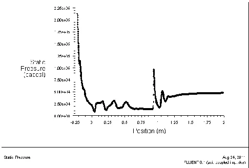
One of the FLUENT advantages is to describe the flow behavior in the models, no matter how complex the fluid flow is. Figure 4 describes the contours of Mach number and figure 5 shows the static pressure profile along the thermocompressor axis.

Fig. 4 contours of Mach number within the thermocompressor

It is clear from the fig. 5 that the high Mach number at the nozzle exit leads to a sudden drop in the static pressure at this area. This pressure is lower than the suction pressure at the suction inlet. So this pressure difference causes the suction steam to enter the suction chamber of the thermocompressor. The suction flow velocity at the entrance is too low, but when it enters the thermocompressor and is mixed with the high velocity motive steam which leaves the nozzle exit, it accelerates through the thermocompressor. The mixed flow reduces its velocity at the diffuser. At this part the static pressure increases gradually with fluctuations. At the converging section of the diffuser the high velocity difference between the motive fluid at the nozzle exit and the suction steam near the wall can create a separate layer.

The high speed of motive steam also acts like a wall and the conditions for choking the suction fluid can be provided. At the specific distance in the throat or at the beginning of the diverging part of diffuser, the flow experiences a normal shock and the static pressure gradually recovers to the discharge pressure value. The flow velocity, on the other hand, decrease to a subsonic level as it travels through the diffuser exit.

B. Effect of operating conditions on thermocompressor performance

1)Effect of back pressure

The effect of the back pressure on the entrainment ratio for the thermocompressor model according to its operating conditions is depicted in fig. 6. The motive and suction pressures are constant while the discharge pressure changes.

According to this picture, there are three regions for the thermocompressor performance: choked flow, unchoked flow and reversed flow. At the choked flow region, the thermocompressor operates with a constant entrainment ratio Rm and increasing in the back pressure does not affect its quantity. At this region both motive and suction fluid are choked and for this reason this is named as double choking region in some literatures. When the back pressure reaches to a point which is called critical back pressure, the Rm starts decreasing until a zero value.

Fig. 6 effect of back pressure on the entrainment ratio

The thermocompressor operates at the unchoked region at this stage. At this region just motive fluid is choked and suction fluid is no longer choked at the diffuser throat. So this region is named as single choking region in some literatures. The point that the entrainment ratio reaches a zero magnitude is named break down pressure. Finally, further increasing in the back pressure causes the thermocompressor to operate at the reversed flow region which the reverse flow phenomena occurs in the suction inlet and results in failure in the thermocompressor operation.

2) Effectof motive steam pressure

Figure 7 depicts the variation of entrainment ratio for different motive pressures varied in the range of 6.5 to 7.5 bar

while the suction pressure is constant. At each case, the performance diagram of the thermocompressor can be divided into 3 regions as discussed earlier. It is clear from the figure that decreasing the motive pressure causes the entrainment ratio to increase but critical back pressure to decrease.

Fig. 7 effect of motive steam pressure on the entrainment ratio

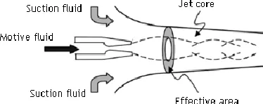
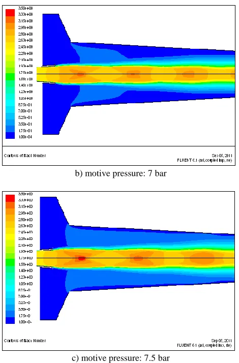
This behavior can be related to the size of jet core and effective area for each operating pressure. These conceptions are shown in figure 8. As mentioned earlier, the jet core of the motive fluid which leaves the nozzle exit plane acts like a wall. The area between this virtual wall and the thermocompressor wall is called effective area.

Fig. 8 conception of effective area

According to the Munday and Bagster theory [24], in the mixing process of the motive and suction fluids in the thermocompressor, these fluids do not mix until their velocities reach the sonic condition. It means that the mixing process starts when the suction fluid chokes. The area where the suction fluid chokes is called effective area.

b) motive pressure: 7 bar

c) motive pressure: 7.5 bar

Fig. 9 effect of motive pressure on the effective area

The smaller jet core gives the bigger effective area and it means that a higher amount of suction fluid can be entered the thermocompressor. In other words, the smaller jet core causes the higher entrainment ratio. The operating pressure can affect the size of jet core and subsequently, the size of effective area and entrainment ratio. As figure 9 shows, the lower motive pressure gives a smaller jet core at the nozzle exit which results in the higher entrainment ratio.

3)Effect of suction temperature

The effect of suction steam temperature on the thermocompressor performance has been illustrated in fig. 10.

Fig. 10 effect of suction temperature on the entrainment ratio

The suction temperature is varied from 63°C to 67°C, while the motive pressure is unchanged. As is clear from the profiles, increasing the suction fluid temperature causes to increase both entrainment ratio and critical back pressure.

C. Effect of geometrical factors on the thermocompressor performance

1) Effect of area ratio

An important geometrical factor which affects the thermocompressor performance is the area ratio between the diffuser throat and nozzle throat, which is defined as:

rA = (dth/dNozz)2 (5)

Where dth is the diffuser throat diameter and dNozz is the nozzle throat diameter. Figure 11 describes how the change of area ratio influences the entrainment ratio. In this investigation three values of 25, 27 and 29 are considered for rA by choosing the diffuser throat diameter of 130, 135 and 140 mm, respectively. At each case the nozzle throat diameter is constant and equal to 26 mm. This diameter for the nozzle throat causes the motive steam to be choked when passes through it. The operating conditions at the boundaries remain constant. In general, when rA increases, it causes to raise the entrainment ratio and decrease the critical back pressure. It should be mention that there is always an optimal area ratio for each thermocompressor based on its operating conditions.

Fig. 11 effect of area ration on the entrainment ratio

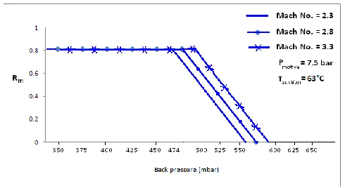
2) Effect of nozzle exit plane diameter

nozzle exit plane. Nozzle with high exit Mach number will have a large exit plane diameter which can obstruct the suction fluid to be entrained. Moreover, high Mach number at the exit of the nozzle may create the noise pollution in the industry where in the thermocompressor operates.

Fig. 12 effect of nozzle exit plane diameter on the entrainment ratio

V. CONCLUSION

Flow behavior within a designed model of a thermocompressor was investigated by using the CFD method and the effects of operating conditions and geometrical factors on its performance were evaluated. It has been already verified that the CFD is an efficient tool to estimate the entrainment ratio ad critical back pressure of the thermocompressor for different operating conditions. It also helps to reveal the phenomena inside the thermocompressor in details. According to the obtained results, for practical purposes, the best way to increase the entrainment ratio for an installed thermocompressor in an industry is to decrease the pressure of motive steam. However, it should be taken into consideration that decreasing the motive pressure will decrease the critical back pressure. Other variables such as increasing the throat diameter or suction temperature cannot be easily applicable for an installed thermocompressor in the industry, even though they increase the entrainment ratio. Results also indicated that increasing the Mach number at the nozzle exit plane does not affect the thermocompressor performance but it will increase the critical back pressure.

NOMENCLATURE dNozz nozzle throat diameter dth diffuser throat diameter g acceleration of gravity vector h specific enthalpy

I identity matrix

k thermal conductivity, turbulent kinetic energy m mass flow rate

P pressure

Rm entrainment ratio rA area ratio

S modulus of the mean rate-of-strain tensor T temperature

t time

U mean velocity u fluctuating velocity v velocity tensor

x general space coordinate Greek letters

ε turbulent kinetic energy dissipation rate μ dynamic viscosity

ρ fluid density τij shear stress tensor υ kinematic viscosity υt turbulent viscosity

σk turbulent Prandtl numbers for k σε turbulent Prandtl numbers for ε

ACKNOWLEDGMENT

This work was supported by the Islamic Azad University, Neyriz Branch, Iran.

REFERENCES

[1] J.H. Keenan and E.P. Neumann, “A simple air ejector”, ASME Journal

of Applied Mechanics, 64, 1942, pp. 75-81.

[2] I.W. Eames, S. Aphornratana and H. Haider, “A theoretical and experimental study of a small-scale steam jet refrigerator”, International

Journal of Refrigeration, 18 (6), 1995, pp. 378–386.

[3] A.E. Kroll, “The design of jet pumps”, Chemical Engineering Progress, 1 (2), 1947.

[4] D.R. Croft and D.G. Lilley, “Jet pump design and performance analysis”, AIAA 14th _{Aerospace Science Meeting, AIAA Paper 76183,}

New York, 1976.

[5] I.W. Eames, “A new prescription for the design of supersonic jet pumps: the constant rate of momentum change method”, Applied Thermal

Engineering, 22, 2002, pp. 121–131.

[6] H. El-Dessouky, H. Ettouney, I. Alatiqi and G. Al-Nuwaibit, “Evaluation of steam jet ejectors”, Chemical Engineering and

Processing, 41, 2002, pp. 551–561.

[7] S.B. Riffat and P. Everitt, “Experimental and CFD modeling of an ejector system for vehicle air conditioning”, Journal of the Institute of

Energy, 72, 1999, pp. 41-47.

[8] M.L. Hoggarth, “The design and performance of high-pressure injectors as gas jet boosters”, Proceedings of the Institution of Mechanical

Engineers, 185, 1970, pp. 755-766.

[9] S.B. Riffat, G. Gam and S. Smith, “Computational fluid dynamics applied to ejector pumps”, Applied Thermal Engineering, 16 (4), 1996, pp. 291-297.

[10] S.B. Riffat and S.A. Omer, “CFD modeling and experimental

investigation of an ejector refrigeration system using methanol as the working fluid”, International Journal of Energy Reservation, 25, 2000, pp. 115–128.

[11] S. Da-Wen and I.W. Eames, “Recent developments in the design theories and applications of ejectors”, Journal of the Institute of Energy,

68, 1995, pp. 65-79.

[12] ESDU (Engineering Sciences Data Unit), “Ejector and jet pump; design for steam driven flow”, Item number 86030, ESDU International Ltd., London, 1986.

[13] E. Rusly, A. Lu, W.W.S. Charters, A. Ooi and K. Pianthong, “Ejector

CFD modeling with real gas model”, Mechanical Engineering Network

of Thailand the 16th Conference, 2002, pp. 150–155.

[14] Y. Bartosiewicz, Z. Aidoun, P. Desevaux and Y. Mercadier, “Numerical and experimental investigations on supersonic ejectors”, International

[15] Y. Bartosiewicz, Z. Aidoun and Y. Mercadier, “Numerical assessment of ejector operation for refrigeration applications based on CFD”, Applied Thermal Engineering, 26, 2006, pp. 604–612.

[16] FLUENT user’s manual, version 6.1, 2005.

[17] S. Aphornratana, “Theoretical and experimental investigation of a combine ejector-absorption refrigerator”, PhD thesis, University of Sheffield, UK, 1994.

[18] T. Sriveerakul, S. Aphornratana and K. Chunnanond, “Performance prediction of steam ejector using computational fluid dynamics: Part 1. Validation of the CFD results”, International Journal of Thermal

Sciences, 46, 2007, pp. 812–822.

[19] S. Vargaa, A.C. Oliveiraa and B. Diaconub, “Influence of geometrical factors on steam ejector performance - A numerical assessment”,

International journal of refrigeration, 32, 2009, pp. 1694-1701.

[20] S. Aphornratana, “Theoretical study of a steam-ejector refrigerator”,

International Energy Journal, 18 (1), 1996, pp. 61-74.

[21] J. H. Keenan, E.P. Neumann and F. Lustwerk, “An investigation of ejector design by analysis and experiment”, ASME Journal of Applied

Mechanics, Sep.1950, pp. 299-309.

[22] GAMBIT user’s manual, version 2.0.4, 1998.

[23] K. Pianthong, W. Seehanam, M. Behnia, T. Sriveerakul and S. Aphornratana, “Investigation and improvement of ejector refrigeration system using computational fluid dynamics technique”, Energy Conversion and Management, 48, 2007, pp. 2556–2564.