Reflection Equations in Exactly Solvable
Models of Statistical Mechanics
Vladislav Fridkin
March 11th, 1999
The work contained in this thesis is my own original research, and any material taken from other references is explicitly acknowledged as such. I certify th at the work contained in this thesis has not been submitted for any other degree.
A c k n o w le d g e m e n ts
I would like to thank my supervisory panel Murray Batchelor, Rodney Baxter and Brian Davies for their assistance and advice during the course of my doctorate degree. Especially I would like to thank my supervisor Murray Batchelor for his fine assistance in all my areas of research.
I would also like to thank Leung Chim, Atsuo Kuniba, Ming Yung and Yukui Zhou for their guidance and collaboration.
It was a pleasure to stay with Kazumitsu Sakai while visiting Tokyo university. I am also indebted to the kind help of Jean-Marie Maillard for my stay at Institut Henri Poincare in Paris, and to Bernard Nienhuis for my stay at Amsterdam University.
Many thanks go out to Sang-up Park, for my stay in South Korea. My warmest thanks go out to my little Phoenix for the photographs during my seminar in Melbourne.
A b s tr a c t
Statistical mechanics strives to bridge the gap between different scales of a particular physical system, i.e., to obtain the properties of a macroscopic system from knowledge of the inter-playing properties of its microscopic elements. To this end, one such method is the use of lattice type models where the properties of the entire lattice are calculated using a knowledge of the interaction between individual edges or vertices. Lattice type models are a simplification of natural systems which are too difficult to solve exactly. However, some important properties of natural systems are the same as those calculated from simplified lattice versions because of universality. Properties such as free energy and entropy are derivable from the partition function. The partition function can be worked out exactly when taking the infinite lattice limit. At this limit only the largest eigenvalue of the
transfer matrix of an integrable model is required. A well used method to find the eigenvalue
is the Bethe ansatz or algebraic Bethe ansatz. Integrability is associated with having a
Yang-Baxter equation in a lattice with periodic boundaries (i.e. toroidal topology). For a
model which has independent boundaries in one direction (i.e. cylindrical topology) the Yang-Baxter equation together with the reflection equation guarantee integrability. These models also have additional surface properties associated with the boundary which are absent in models with periodic, or trivial boundaries.
In this thesis methods of solving the reflection equation and properties of the aforemen tioned models with non-trivial boundaries are examined. A new framework for boundary integrability for interaction-round-a-face models is introduced as a natural extension of that for the vertex models. In particular the dilute Al face model and the series of
L ist o f P u b lic a tio n s
The bulk of original material is contained in chapters 3, 4 and 5. The framework given in chapter 2 for boundary integrability is an extension of collaboration with Murray Batchelor and Yukui Zhou.
The results of chapter 3 appear in the paper:
• M T Batchelor, V Fridkin and Y K Zhou, An Ising model in a magnetic field with a
boundary, J Phys A 29 (1996) L61-L67.
The results of chapter 4 appear in the papers:
• M T Batchelor, V Fridkin, A Kuniba and Y K Zhou, Solutions of the reflection
equation for face and vertex models associated with An \ Bn \ Cn \ D n' and A n \
Phys Lett B 376 (1996) 266-274.
• M T Batchelor, V Fridkin, A Kuniba, K Sakai and Y K Zhou, Free energies and
critical exponents of the B n \ Cn^ and Dn'1 face models, J Phys Soc Jap 66
(1997) 913-916.
Ongoing research of chapter 5 is to appear in the papers:
• V Fridkin and M T Batchelor, A tiling model associated with the A ^ vertex model
with non-trivial boundary conditions, Currently in preparation.
• V Fridkin, Non-diagonal solutions of the reflection equation for the IRF models as
sociated with affine Lie algebras, Currently in preparation.
C ontents
1 F rom p h a se tr a n s itio n s to th e Y a n g -B a x te r e q u a tio n 1
1.1 Modern statistical mechanics ... 2
1.2 The Yang-Baxter equation ( Y B E ) ... 11
2 T h e R e fle c tio n E q u a tio n and D o u b le R o w T ra n sfer M a tr ix 21 2.1 Surface free energy and critical e x p o n e n ts ... 21
2.2 The reflection equation (RE) ... 22
2.3 Properties of the RE and s o lu tio n s ... 29
3 T h e A B F and d ilu te Al m o d e ls 36 3.1 Solving for diagonal solutions to the IRF SOS models ... 37
3.2 Surface critical exponents of the dilute Al m o d e l... 47
4 M o d e ls a s s o c ia te d w ith th e A ffin e Lie A lg e b r a s 50 4.1 Unrestricted models ... 51
4.2 Face weights of the B n \ C n \ Dn'1 and m o d els... 54
4.3 Boundary weights... 57
4.4 Restricted m odels... 68
4.5 Free energies and Critical e x p o n e n ts ... 69
5 T ilin g M o d e ls 77 5.1 Bulk and boundary weights of the A^ m o d e l... 78
5.2 Boundary vertices ... 82
5.3 Solutions of the RE for A face m o d e ls ... 86
C h a p te r 1
F ro m p h a se tr a n s itio n s to th e
Y a n g -B a x te r e q u a tio n
I
ntroductionThis chapter is devoted to a historical introduction of the work that precedes this thesis and forms the basis for work with the reflection equation. Various nomenclature required later is introduced and parallel fields are touched upon.
S
ummaryO Modern statistical mechanics
Phase transitions and critical phenomena TYie partition function
Critical exponents Lattice and face models The six-vertex model
Partition Sums: from a vertex, to a row, to a lattice Solving for the partition function
The commuting transfer matrix method
O The Yang-Baxter equation (YBE)
The eight-vertex model: toroidal boundary conditions Relationship between u, v and w
Matrix inversion method: Eigenvalue calculation Boltzmann weights and YBE in R-matrix form SOS Models and Intertwiners
RSOS Models: The ABF Model Solutions of the Yang-Baxter equation
2 F ro m p h a s e tr a n s itio n s to th e Y a n g -B a x te r e q u a tio n
T
heD
etails1.1
M o d e r n s t a t is tic a l m e c h a n ic s
Theories of nature are ever changing. One of them, statistical mechanics, has branched out from its beginnings in thermodynamics, when the Newtonian idea of the universe was pervasive, into the realm of quantum mechanics as well as conformal field theory, knots and braids and the representation theory of quantum affine algebras.
In statistical mechanics, researchers developed models to try to understand phase transitions and critical phenomena. Initially these models were based upon continuum theory, later more refined models taking into account the atomic nature of m atter and quantum mechanics appeared. Numerical calculation for the properties of these atomic based models is very testing of modern computational methods and resources. Thus analytic and exact solution seems an attractive option if it is possible. This has been possible for a small but growing number of models. The techniques of exact solution vary, but the technique of transfer matrices and Yang-Baxter equation remains at the forefront of these since its use in the solution of the eight-vertex model. With expanding techniques come more general models. Solvable models with non-trivial boundaries is a natural generalisation. In this thesis, new outgrowth is explored from this branch of exactly solvable models in statistical mechanics with boundaries which builds upon the transfer matrix technique to involve what is called the reflection equation. We now turn to a more detailed exposition leading up to the reflection equation.
P h a s e t r a n s itio n s a n d c r itic a l p h e n o m e n a
The familiar states of m atter are solid, liquid and gas. A material may be induced to undergo a phase transition from one state to another by accompanying changes in conditions such as temperature, pressure, volume and external magnetic or electric field. Freezing, condensation, melting as well as ferromagnetic phase transitions at the Curie temperature are common examples in everyday life and physics. Statistical mechanics studies systems exhibiting such phase transitions and especially the critical phenomenon which identifies them. Through solving for the properties of critical phenomenon of models which exhibit phase transitions it is believed that the understanding of such phenomenon in nature and associated properties of natural materials advances. Mathematically, in statistical mechanics, this translates into solving for the critical exponents and thermody namic functions using just the knowledge of microscopic properties of the components of the system. The first step in the realisation of this is through the partition function.
T h e p a r titio n fu n c tio n
The probability of a discrete system (a system that can be one of a number of discrete number of states) being in the state o was given by Boltzmann
P(a)
= i e- £(<?)/*T
(1.1)
Zj
where £(cr) is the energy associated with the state a and A:,T are Boltzmann’s constant and temperature respectively. The normalisation Z, introduced by Gibbs [40] , is called
1.1 M o d e r n s t a t is t ic a l m e c h a n ic s 3
the partition function (Zustandsumme or sum-over-states in German) and is the generator of various thermodynamic functions. It follows th at
Z = Y , e~£{<,)/kT (1.2)
G
and the expectation value X —< |A(cr)| > of some macroscopic property is
I = V x ( a ) e - W T (1.3)
G
from which follow expressions for internal energy U, free energy F and entropy 5
U = k T 2^ Tln Z
F = - k T l n Z (1.4)
S = k (T $ r + l)ln Z
Critical exponents
Critical phenomena are characterised by the singularities of thermodynamic functions and occur at what are called critical values of the temperature, pressure, volume and so on1. It is expected that the singularities will be simple positive exponents called critical
exponents. Taking the common example of critical tem perature Tc of a system, we have
under the translated and normalised temperature
t = (T — Tc) / T (1.5)
the following definitions of critical exponents ce, /3, 7, 7', <5, /u, p! and u
fsingX0, T) t2-a t —y 0,
M0(T) l - t ) ß t —y 0 ,
X(0,T) r 7 t o+ ,
H ) - y t —y 0 ,
M ( H ,T C) H l' s H -* 0,
s(T) r>*/ i - t r t —^ 0 ,
f(0 ,T ) r " t -> 0+ , t — 0 ,
ffW r s j r — d+2 — ri1 ?
(1.6)
where f sing.(H ,T ) is the singular part of the per site or intensive free energy and H is the magnetic field strength. The other functions are briefly magnetization M( H, T ) ,
susceptibility x ( H , T), interfacial tension s(T), correlation length £( H, T) and correlation
function g(r) which is a function of vector distance r between two particular spins of a
system and d is the dimensionality of the system. These critical exponents are believed to
4 F r o m p h a s e t r a n s it io n s t o t h e Y a n g - B a x t e r e q u a t io n
be related. The use of scaling arguments gives the following predictions which agree well with experimental and theoretical results:
a + 2ß + 7' u = z/, (2 - rf)v
[L + V
du
2
7
2 - a 2 - a
(1 .7 )
Going beyond these predictions, the use of lattice models to confirm these scaling relations and derive the values of the critical exponents exactly is a major goal of exactly solvable model theory. The justification for why the critical exponents of a simple lattice model and ‘real’ or ‘natural’ system should be the same goes under the heading of universality. Briefly, universality is the supposition that the critical exponents are independent of the complexities of the Hamiltonian of a system, only depending upon its symmetries and the dimensionality of the system. This allows us to choose and try to solve the simplest model in the same universality class of the system we wish to investigate. There are also experimental systems which are two-dimensional and hence provide ample justification in themselves for the investigation of two-dimensional models.
L a ttic e a n d fa ce m o d e ls
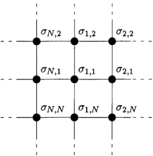
If not the first to be investigated, then at least the most intensively studied model from which the concepts of exactly solvable models originate is the Ising model first proposed by Lenz (1920) and then investigated in 1-D by Ising [50]. It is the only model, so far, for which the complete eigenspectrum has been in general solved explicitly. The model is based on a lattice of spins cra = ±1 where a is a positional labelling defining the lattice, with interaction energies — £(<*, a ')a Qcrai and energy contributions —Hcra due to an external magnetic field. By Dyson [32], no phase transitions exist for the 1-D model if all the interactions are finite. However the 2-D model exhibits phase transitions
[image:11.526.192.341.471.623.2]^ N , N ^ <?1,N ^ ° 2'N
Figure 1.1: T he O nsager lattice, a 2-D Ising model. (Here w ith toroidal boundary conditions.)
for finite interactions as first shown explicitly in Onsager’s solution [76]. It is believed that qualitatively the entire class of models with finite interactions will lead to the same
1.1 M o d e r n s t a t i s t i c a l m e c h a n ic s 5
phase transitions, the difference being only to the class of models with infinite range interactions. This convenience allows us to choose the simplest finite interactions WLOG. The first exact solution of the 2-D Ising model (H = 0) was by Onsager (1944) using the method of irreducible representations of a related matrix algebra to find the eigenvalues of the transfer matrix [76]. For two decades after no new major results were obtained except mainly the simplifications of the methods used [57]. Onsager’s lattice consists of spins <Ja,ß at coordinates (a, ß) of a 2-D lattice. The interaction energies are nearest neighbour which means only energies associated with adjacent spins in the x-axis or y-axis contribute (taking the usual rectangular coordinate system). Furthermore, taken to be position invariant the total energy can be expressed
£ = ~ —H (1-8)
j,k j,k j,k
where — £x ( — £,y) is the energy associated with two nearest neighbours spins adjacent along the x-axis (y-axis). Unfortunately the Ising model was found to belong to a restrictive class of free-fermion models which are limited to solutions within their own class. The six-vertex model broke out of this restriction.
T h e six -v e r te x m od el
The six-vertex model was first solved by Lieb [66] using the Bethe ansatz method. The six-vertex model is an ice-type model defined by the ice rule proposed by Slater [81] on the basis of electrical neutrality in the vicinity of an oxygen atom in ice. In ice, water molecules
(H2O) join due to polar forces to form a lattice in which every oxygen atom is surrounded
by four hydrogen atoms. This concept is translated into a 2-D square lattice where each vertex represents a fixed oxygen atom and each edge represents the position of a hydrogen ion with two allowable states. These two states, each represented by an arrow, are common to each edge of the lattice and represent the hydrogen ion being symmetrically close to one or the other oxygen atom common to that edge, the arrow pointing in the direction of the closer oxygen atom. Each vertex can thus have sixteen allowable configurations of the edges immediately surrounding it. The ice-rule imposes th at arrows pointing into a vertex balance those pointing out. With this rule we are limited to six configurations:
Figure 1.2: Arrow configurations, energies and line representations
[image:12.526.158.401.523.608.2]6 F ro m p h a se tr a n s itio n s to th e Y a n g -B a x te r e q u a tio n
remains constant along the vertical edges. We can also take diagonal boundary conditions which also have this conservation property (with every second row ‘twisted’ with respect to the six configurations shown above as will be explained in more detail later). This conservation property was vital to the technique of the analytic Bethe ansatz.
Figure 1.3: Periodic boundary conditions (left) and diagonal boundary conditions (right) for the six- vertex model
Before continuing with the partition function of these particular models, let us look first at the concepts of partition sums for an arbitrary lattice model.
P a r titio n S u m s: fro m a v e r t e x , to a r o w , to a la ttic e
Let our lattice be of dimensions M x N as indicated above. Take any row of this lattice then it has N edges above and below, a left edge and a right edge. Let us think of the bottom (top) edges as a cumulative edge with a cumulative state being an ordered list of states of its member edges. Assume that it is a 2-state model WLOG. Summing along the horizontal edges that lie between the vertices, a row can be thought of as a cumulative vertex with bottom (top) edge having 2N states and left (right) edge having 2 states.
Figure 1.4: Horizontal dashed edges are summed to give a cumulative vertex on the right with b =
{ bi , 62 , . . . , 6m)
The partition sum Z j of this cumulative vertex can be derived naturally from consid ering its constituent vertices and their individual states
ZT{a,a'\b, b') = exp[-(m i(crT)ei + m2(crT)e2 + . . . + rn6{aT)e6)}
<77'(a,a, |6,6 , )
where mz is the cumulative vertex state crj dependent number of constituent vertices in state i. We can define a two-dimensional vector space V2 associated with the horizontal
edges and a 2jV-dimensional vector space V2n associated with the vertical edges. From this point it is convenient to identify the two states of an edge, thick and thin line, with + and — respectively. The row of edges or cumulative vertex can then be associated with
[image:13.526.129.389.150.247.2] [image:13.526.149.383.453.511.2]1.1 M o d e r n s ta t is t ic a l m e c h a n ic s 7
a monodromyoperator on the tensor product V2 <S> V2n. This operator can be represented
as a monodromy matrix subdivided into four blocks by the states of the horizontal edges. Let the entries of this matrix being partition sums Z j associated with each state of the cumulative vertex
The diagonal blocks D++ and D__ correspond to periodic boundary conditions, i.e., when the horizontal edge states agree. For line conserving models such as the six-vertex model, these diagonal blocks have a diagonal block structure if one groups the vertical cumulative states according to how many thick lines they contain. This is because (c.f. above) for periodic boundary conditions the number of thick lines is conserved from one row of vertical lines to the next. There is a natural extension of the notion of monodromy operator and matrix to the entire lattice. In this case all of the internal edges are summed, horizontal and vertical, and only the boundaries determine the partition sums. For a two state (per edge) model the operator acts on V2m (g) V2n. It is clear that the partition function for a vertex model with toroidal boundary conditions is the trace of such a matrix. For a single vertex, this notion is immediate and the operator and matrix are commonly referred to in the vertex terminology as the R-matrix. To unify this common idea at the different scales of vertex, row (or column) and lattice, here it is proposed to call these partition matrices with symbols Z r,c and {Zr,c} as described in figure 1.5.
b'
a a'
b
b'
I a'
b
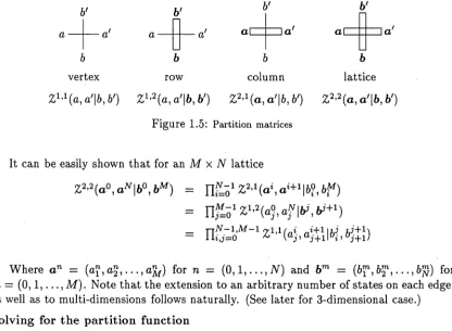
[image:14.526.65.481.376.681.2]vertex row column lattice
Z1,1^ , a'|6, b') Z1’2(a, a'|6, 6') Z2,1(a, a'|6, b') Z2,2(a, a'|6 , b')
Figure 1.5: Partition matrices
It can be easily shown th at for a n M x i V lattice
Z
^ ( a ° , a N \b°,bM) =n ' l y Z 2' V , a ,+1|6?,6ff)
= n ^ ö I Z1'2(a»,af|fr>',V+1)
Where a n = (a™, a2, . . . , a\j) for n = ( 0 , 1 , . . . , N) and bm = (6™, b2l) . . . , 6-y) for m = ( 0 ,1 ,..., M). Note that the extension to an arbitrary number of states on each edge, as well as to multi-dimensions follows naturally. (See later for 3-dimensional case.)
Solving for the partition function
8 F r o m p h a s e t r a n s i t i o n s t o t h e Y a n g - B a x t e r e q u a t io n
function directly using combinatorial arguments and Pfaffians, however this only applies to a limited range of models (such as the Ising, dimer and free-fermion models).
Of the transfer matrix methods, the fermion algebra method was used by Onsager [76] and others to completely determine the spectrum of the transfer matrix for the Ising model. However, it too is limited to the Ising model and free-fermion case.
The other transfer matrix methods are not limited in this way
P a r titio n fu n c tio n s o lu tio n m e th o d s in v o lv in g tr a n sfe r m a tr ic e s
1. Bethe Ansatz
2. Commuting Transfer Matrix 3. Matrix Inversion Relation 4. Corner Transfer Matrix
The concept of a transfer matrix depends upon the method used, however one can, given appropriate boundary conditions, think of any partition sum, Z771’71, as a transfer matrix. In method 2 the transfer matrix in question is usually Z1,2 and called the row transfer matrix, first introduced by Kramers and Wannier [60]. For method 4, originated by Baxter [14], the entire lattice is broken up into four sub-lattices called corner transfer matrices of type Z2,2. In this thesis the focus is upon the commuting transfer matrix method, along with the Bethe ansatz and matrix inversion methods to a lesser degree. To begin illustrating the commuting transfer matrix method, let us return once again to the six-vertex model.
T h e c o m m u tin g tr a n sfe r m a tr ix m eth o d :
s ix - v e r t e x m o d e l w ith to r o id a l b o u n d a r y c o n d itio n s
Consider the calculation of the partition function, Z, which mentioned earlier is the generator of various thermodynamic quantities. For the six-vertex model (lattice size M X N) we have
where n; is the lattice state a dependent number of vertices in state i. Thus we always have the consistency condition ^ r i i = N X M. It is clear from line conservation that
7i5 = tiq (as is ms = me above for each row) and so we may take €5 = €e WLOG. It is also conventional to take e\ = e2 and €3 = c4. From the above section on partition sums, we have th at the partition function for toroidal boundary conditions is given by the trace of the partition matrix
6
Z = ]T e £M /tT , £(<r) = (1.9)
•Z = H a , 6 Z 2'2(aa | 6 , 6)
= T r { Z 2’2( a ° , a N \ba,b
(1.10) M - l
j=o a°=aN
1.1 M o d e r n s t a t i s t i c a l m e c h a n ic s 9
Defining the transfer matrix for toroidal boundaries to be
T j =
£ z 1'2(a“,a~|6>,0'+1) ( M l )« ; = <
we have the usual expression for the partition function in terms of a product of row transfer matrices
M- 1
Z ^ T r l l T , (1.12)
J = 0
Note th at the cumulative vertex (1.4) taken with periodic horizontal boundary conditions is the transfer matrix here. The next step in the commuting transfer matrix method is using the algebraic result that a commuting family of matrices can be simultaneously diagonalised, i.e., there exists a matrix P satisfying P T = P ~ lsuch th at for the commuting
family {Tj} we have
P T i P 7 = D, V T , e { T j } (1.13)
where Dt is a diagonal matrix consisting of the eigenvalues of 7). Substituting the expression (1.13) into (1.12)
N- 1 2n N - l
Z = T r
n D;
=£ n **
d-14)
j=o k=l j=0
recalling that for the six-vertex model there are 2 states to every edge and thus N ordered edges have 2N states.
Thus the task of calculating the partition function reduces to th at of determining the eigenvalues of the transfer matrices if they form a commuting family. Also important is the fact th at the commutation property of the transfer matrices aids in the calculation of the eigenvalues, as will be explained.
For now let us look into the Bethe Ansatz method of finding these eigenvalues.
T h e B e th e A n sa tz m eth od
The Bethe Ansatz method was first used to solve the one-dimensional Heisenberg model [22]. Lieb then used it to solve the six-vertex model [66]. This is briefly discussed here to illustrate the method.
It was noted earlier th at the conservation property of the number of thick lines (1.3) from row to row was necessary for the use of the analytic Bethe Ansatz.
Due to the incoming state bz and outgoing state 6,-+i of transfer matrix T) having the same number of thick lines n, one can order the states {bj} so that all the transfer matrices have a block structure, each block being determined by n. This reduces the calculation of the eigenvalues to the smaller blocks of the transfer matrix. Also since the blocks are labelled by n, this motivated the search for a relationship between the eigenvalues and n. The Bethe Ansatz, or guess, for the eigenvectors followed along these lines.
9n{x) = Ap Y[ g { z Vl,Xi) , g(z, x) = zx (1.15)
10 F r o m p h a s e t r a n s i t i o n s to t h e Y a n g - B a x t e r e q u a t io n
where the sum is over all permutations p of 1, . . n and the ordered positions of the n thick lines are denoted by x. If we define the Boltzmann weights = exp(— Si/kT) and set
a = U>1 = 2, b = LO3 = (J4, C — Co>5 — UJQi (1.16)
a2 + b2 - c2
2 ab (1.17)
then the result of the Ansatz after solving for the Ap gives the eigenvalue An for the n-block
An = aNL n (a, b , z *) + 6AI n(6, a, z), L n{a,b,z)
M
-pr 26 A — a — b Z{b - a z i (1.18)
and the Zi are determined by the Bethe Ansatz equations
n
2A = ( - l ) n_1 Sji/sij, Sij = 1 - 2Azi + ztZj (1.19)
3 =1
Similar formulas are obtained for arbitrary Boltzmann weights uj%. Unfortunately these Bethe Ansatz equations have not been solved in general for finite n and N unlike the case of the Ising model for which the entire spectrum is known for each N . They have been solved for the largest eigenvalue in the thermodynamic limit, i.e., when N —> oc. Some correlation lengths (mass gaps) and finite-size corrections for various eigenvalues have also been calculated.
Since zt are determined by A, the eigenvectors (1.15) depend on the Boltzmann weights only through A. Thus each value of A defines a family of commuting transfer matrices
(since having commutation is equivalent to having the same eigenvectors).
In terms of trigonometric functions the following parametrisation satisfies (1.17)
a = sin(A — u), b = s'mu, c = sin A, A = — cos A (1.20)
where A is taken constant and u may vary from one transfer matrix to the next. (A simple way to arrive at this parameterisation is to realise that (1.17) is an equation for a triangle with sides having length a, 6, c where A, u are angles opposite the sides c, b respectively.)
W hat has occurred is that the method outlined above, uses a simplification of the eigenvalue calculation in order to determine a class of Boltzmann weights. This in effect works backwards from the concept of using the properties of the small to find the properties of the large.
As mentioned previously, the analytic Bethe Ansatz works for line conservation. There is an alternative method, which solves for the Boltzmann weights as above, however does not depend upon line conservation and works for a larger class of models. This entails the use of the Yang-Baxter equation.
1.2 T h e Y a n g -B a x te r e q u a tio n (Y B E ) 11
1.2
T h e Y a n g -B a x te r e q u a tio n (Y B E )
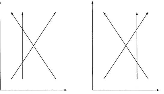
Before the YBE came to play a recognised role in statistical mechanics through the work of Baxter and Yang, it was known in the form of the star triangle relation at least as far back as 1945 by Wannier in his work on the honeycomb dual to the Ising model and even by Onsager prior to his solution in 1944 according to Baxter [82]. In another context, the YBE was hinted at in the work of McGuire [67]. Using Bethe-type wave functions, it was shown that the Y-particle 5-m atrix factorises into the product of two-particle 5-matrices with the YBE being a resulting implicit consistency condition illustrated in figure 1.6.
Figure 1.6: “. . . as far as the outgoing waves are concerned, it does not matter which of the two possible diagrams is used, for both give the same result. ”
The first explicit mention of the YBE was by Yang [86] in work using the nested Bethe ansatz, again appearing as a consistency condition. Later it found importance in statistical mechanics through Baxter’s solution of the eight-vertex model [12]. This led to the coining of the name ‘Yang-Baxter equation” by Faddeev’s group in St. Petersburg according to [16],
The YBE in lattice theory is part of the commuting transfer matrix method. If transfer matrices are made up of Boltzmann weights that satisfy the YBE then they commute. To illustrate this in more detail along with necessary definitions, the eight-vertex model is used as an example.
T h e eig h t-v e r te x m odel: to roid al b ou n d ary con d ition s
The eight-vertex model is made up of the six-vertex model vertex configurations plus a sink and a source. The Boltzmann weights uq, . . . , wg are in general distinct and depend upon their site in the lattice.
Following on from the six-vertex case define
a = UJ\ = U 2 , b = U)3 = U > 4 , C = CÜ5 = u>6, d = OJj — UJg, (1.21)
Motivated by the six-vertex model results, take a priori that the Boltzmann weights
a ,b ,c,d vary only from row to row and consider the commutation of two row transfer
[image:18.526.135.408.211.368.2]12 F ro m p h a s e t r a n s itio n s to th e Y a n g -B a x te r e q u a tio n
\ t
r *7
UJi UJ2 (x>3 CJ4 U 5 IPß CP7
+
— —+
+
— -+
+
+
- -+
+
- -+
_ _+
+
_ _+
+
—+
+
— [image:19.526.65.455.63.157.2] [image:19.526.136.384.319.436.2] [image:19.526.132.377.537.580.2]- +
Figure 1.7: Arrow configurations, Boltzmann weights and associated plus-minus configurations
between the transfer matrices and are not to be regarded as any particular parameterisa- tion.
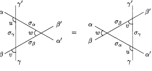
In contrast to the Bethe-Ansatz method, Baxter found that the commutation of T( u) and T(v) can be established directly with the use of the YBE. The YBE is made up of a sum of products of these weights. The internal states <7a ,<7/j,«77 are summed (as in figure 1.4 indicated with dashed lines) and the external edges are identified as shown in figure 1.8. The little curve between the edges represents orientation so th at this equation
ß'
cd
Figure 1.8: Yang-Baxter equation for the vertex model
is independent of rotation unlike the representation in figure 1.7; there the little curve is determined to lie in the lower left quadrant which is usually the case when it is omitted.
It is also useful to have an inverse set of weights in the sense of figure 1.9.
a
ß
Oi'
ß'
a
= S a a ' b ß '
ß
a
ß
Figure 1.9: Inversion for the vertex model
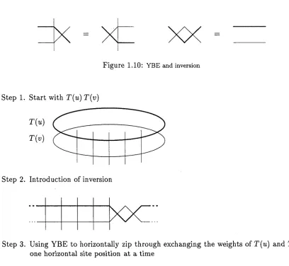
To avoid excessive labelling, a thick and thin line shall represent the horizontal edges of the vertices of T( u) and T(v) respectively. The YBE and inversion are then simplified as in figure 1.10. The YBE and inversion are enough to allow commutation; the steps shown here (with N = 5 WLOG)
1.2 T h e Y a n g - B a x t e r e q u a t io n ( Y B E ) 13
Figure 1.10: YBE and inversion
Step 1. Start with T { u ) T { v)
Step 2. Introduction of inversion
Step 3. Using YBE to horizontally zip through exchanging the weights of T(u) and T(u) one horizontal site position at a time
X
Step 4. Periodic boundary conditions lead to inversion (mirror of th at introduced)
x>c:
Step 5. End with T( v ) T ( u )
The condition for [T ( u ) , T ( v)] = 0 is reduced to solving the YBE which Baxter did so by considering symmetries to reduce the number of equations from sixty four to six. They are satisfied if the quantities A and T are constant from row to row, i.e., A(u) = A(u) and
r(w)
=r(u),
whereA = a2 + b2 - c2 - d2 ab
ab — cd
14 F rom p h a se t r a n s itio n s to th e Y a n g -B a x te r e q u a tio n
These conditions lead to the parameterisation of a, b, c, d in terms of entire functions involving elliptic functions (1.25)
a{u) = $ 4 (u) $i( A — u )
0 iW 0 4(O) &(«)
$1 (ti) 7^4 (A — u)
0i( A ) 0 4 (O)
^ 4 (w) ^4 ( A — W)
794(A)^4(0) d ( w )
( w ) ^ i ( A — w )
(1.23)
where the u dependence is now explicitly defined and A and T depend only on A which is therefore constant for each family of commuting transfer matrices.
A = *i(2A) ( *i(A) i94(A)
r =
l?4 (2A)
0 , ( A ) / ’ '
<^(A ) + 0?(A )
The standard elliptic theta functions of nome p, |p| < 1, are defined as
OO
(u) = (u, p) = 2p1/ 4 sin u jQ ^1 — 2p2n cos 2u + pAn^j ^1 - p2n^j
n — 1 oo
$4(u) = tf4(u,p) = n (l ~ 2p2n_1 cos2u + p4n~2) ( l - p2n) .
(1.24)
(1.25)
n = 1
Under appropriate normalisation conditions, these functions reduce to trigonometric func tions and the weights (1.23) and A (1.24) reduce to the six-vertex weights (1.20) and A
(1.20).
R elationship betw een u, v and w
By symmetry the intertwining weights a ( w ) , . . . can also satisfy the above solutions (1.21). Substituting these solutions into the YBE one obtains the following relationship WLOG
w = u - v (1.26)
This is commonly referred to as the difference property.
M atrix inversion m ethod: Eigenvalue calculation
If we take v = A + u, then the following inversion relation is found to hold for the eigenvalues of the transfer matrix
#i (A — tt)#i(A + w)#4(A - u)#4(A + u) A(w) A(A + u)
*?(AK(A) (1.27)
which can together with further symmetry properties be solved to determine the free energy, taking into account some analyticity requirements.
B oltzm ann w eights and Y B E in R-m atrix form
It is historically common to use the matrix element term form representation and the
operator form representation of the YBE. These are now discussed for a general vertex
model.
1.2 T h e Y a n g - B a x t e r e q u a t i o n ( Y B E ) 15
Define the non-zero R-matrix elements by
ß'
,Ot ß'
ßa' (u) = XT Oi'
ß
(1.28)
where the states on the edges corresponding to allowable vertex configurations are labelled by Greek letters a, (where a , £ {+, —} for the six-vertex and eight-vertex model) and the vertex picture represents its Boltzmann weight. The dependence upon lattice site is encoded into the dependence on u. The familiar term form representation of the YBE
E
(
u
)K;Z‘
m
=
E
rvsw
K ’JW K 'I
i
?)
& Ot ß *y & Ot ß
can then be read off figure 1.7. If we were to use the preceding u dependence relationship then we have w = u — v. The exponential of these is sometimes used which gives a multiplicative property. However for the Chiral Potts model, which has no such property between the parameters, the parameterisation is much more complicated.
Recalling the operator interpretation of the cumulative vertex (on page 6), the ill- matrix has a corresponding R-operator R xy : Vx <g> Vy —> Vy <S> Vx (which is usually just called R-matrix as well). The operator R xy = PxyR xy, where Pxy{a (g> b) = b <g> a is the
permutation operator, is also commonly used. Here the following convention is taken
x y
Rxyi'U') — X y
y
(1.30)
In this notation the operator forms of the YBE are
Rn{u)R\3{v)R23{w) = R23{w)Ri3{v) Rn {u )
(1.31)
R23(v) R U {u) R 23{w) = R i 2 M R 23( u )R i2(u)
where the action here is on V\ (g> E2 <g> V3 and R xy acts trivially on all subspaces except Vx and Vy.
SOS M o d els and In tertw in ers
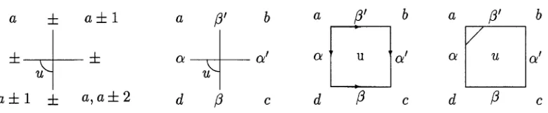
In vertex language the states on the edges correspond to the possible states of hydrogen in ice in the six-vertex model. Labelling these states + and - as in figure 1.7 these may also be interpreted as height differences in the following sense: Subdivide a plane into four quadrants and assign a number a to the top left quadrant and numbers 6, c, d to the others in a clockwise direction. Allow the values of 6,c, d to be such th at neighbouring quadrant numbers differ by ±1. This allows six possible configurations of a, 6, c, d. Taking
a = d — a, a' = c — b, ß = c — d, ß' = b — a we obtain a one-one correspondence with the
16 F rom p h a se tr a n s itio n s to th e Y a n g -B a x te r e q u a tio n
instead of the middle of the faces. As illustrated in figure (1.11) we can represent the ‘direction’ of change by arrows or a ‘tag ’ in the corner indicating the ‘flow’ of arrows away from a. If we interpret the numbers a,6, c, d as heights and the edges as joining these heights then we obtain a discrete manifold in three dimensions. This can be thought of as representing an interface between two solids leading to the name Solid-On-Solid or SOS model. For SOS models it is common to either label the heights or specify one height
a ± a ± 1 a ß ' b a ß' b a ß' b
± _ £
--- ± Ckf --- ---a' a u V a
/ u
a ± 1 ; - a, a ± 2 d ß c d > c d ß
Figure 1.11: A two sta te { + , —} exam ple illustrating six-vertex correspondence, general vertex repre sentation, arrow face representation and tag face representation w ith a = d — a, a 1 = c — b, ß = c — d, ß 1 — b — a
and the height differences around the square. These configurations can be associated with Boltzmann weights which in this scheme are called face weights and represented in (1.32)
basic functional face (arrow) face (tag) vertex
(1.32)
For this reason another name for these models is Interaction-Round-a-Face or IRF models. The conventions for labelling as well as names commonly used are:
heights a, 6, c , .. . first few Latin letters
vector differences a ,/? ,7 , . . . Greek letters (1.33)
spectral parameters u, v, w ,. . . last few Latin letters
One of the first of the IRF models investigated is the eight-vertex SOS model which is explained briefly below.
It is clear that the ice-property, i.e., conservation of lines property of the six-vertex model translates into a physical requirement for the IRF models, namely a -f ß = ß' -f a'. Through the use of intertwiners (1.34) Baxter was able to relate the eight-vertex weights with those of an SOS model and use this conservation property in order to build up Bethe Ansatz equations for the eigenvalues. The intertwiners are represented and defined as
if (1.34)
[image:23.526.65.456.189.270.2]1.2 T h e Y a n g - B a x t e r e q u a t io n ( Y B E ) 17
having no state dependence on the vertical edges. These intertwiners link the face weights of the SOS model to the weights of the vertex model through the face-vertex intertwining equation
(1.35)
where the internal height d and edge states cra , crp are summed over. In term or functional representation, this equation can be read from (1.35) to give
ß u — v
=
Y
R l ? S u - v)v > ( < 7 0a° a , V ß \ 0
(1.36)
which relates the following eight-vertex SOS model weights to th at of the eight-vertex model (1.23) under normalisation
W
W
a ± 1 a
l « a 1
(
a a =p 1la ± 1 a
d i (A — u) / a a i l \ d" i u) (A) y a i l a J $i(aA + uq j
di(u) /^ i((a + 1)A + w0)fli((a - 1)A + w0) \ 1/2
#i(A) V d\ (aA + u;0) J
(1.37)
where wo is an arbitrary constant. Either explicitly or through the above face-vertex inter twining equation, one can verify that these weights satisfy the face Yang-Baxter equation
18 F r o m p h a s e t r a n s i t i o n s t o t h e Y a n g - B a x t e r e q u a t i o n
R SO S M odels: T h e A B F M o d el
In principle, the possible number of states for a finite-size lattice with SOS weights
seems limitless. However it was found th a t for particular restrictions, i.e., particular values
of c^o and A these weights closed in am ongst themselves. For example choosing
= 0 A = (1.39)
we obtain
= 0 unless a, 6, c, d E { 1 , . .L}. (1-40)
where L E Z+. The first non-trivial weights are for L = 3, for which we have six distinct faces. This model is called the ABF-model after Andrews Baxter and Forrester [4j. In
general, SOS models restricted in this way are called Restricted-Solid-On-Solid or RSOS
models. An infinite hierarchy of RSOS models can be generated from an SOS model
depending on L. W hat is particularly interesting is th a t for L = 2,3 above, we obtain the
Ising and hard hexagon model respectively which was the first connection between these models and the eight-vertex model.
S olu tion s o f th e Y a n g -B a x ter eq u ation
So far the Ising, six-vertex, eight-vertex and ABF models have been discussed briefly. There are however a m ultitude of other solutions th a t have been found. These are sum marised in the following table, which is by no means exhaustive.
Year Solutions of Yang-Baxter Equation
1967 trig. (Yang) [86]
1972 8-vertex model ell. (Baxter) [12]
1973 8-vertex SOS model ell. (Baxter) [13]
1978 Gross-Neveu model trig. (Zamolodchikov2) [91]
1981 Z n+i X Zn + 1 Belavin model ell. (Belavin) [21]
19-vertex model trig. (Izergin & Korepin) [51]
1984 ABF Model ell. (Andrews, Baxter & Forrester) [4]
1986 trig. (Jirnbo) [53]
1987 trig. (Bazhanov) [18]
Graph state models trig. (Pasquier) [77]
1992 Dilute Al models ell. (W arnaar, Nienhuis & Seaton; Roche) [83, 78]
1 .2 T h e Y a n g - B a x t e r e q u a t io n ( Y B E ) 19
Methods primarily used in order to solve the YBE are given here briefly.
M ethods for solving the Y ang-B axter equation
1. Symmetry conditions
2. Quantum Groups
3. Already integrable models
4. Pasquier’s adjacency matrix
5. Fusion
6. Intertwining relation
Sym m etry conditions are those such as the ‘ice-rule’ where the form of the solution is specified initially and the resulting reduced set of equations is solved directly. In some cases differential equations are set up from these by partial differentiation WRT v and then letting v = 0.
Quantum Groups or Zamolodchikov’s algebra has the YBE as an associativity con dition of this algebra. Through representations of the algebra one can obtain the solutions of the YBE.
A lready integrable m odels with families of commuting transfer matrices constructed without the use of the YBE can be the basis for new solutions.
P asquier’s adjacency m atrix method exploits the fact that the YBE for the critical (trigonometric limit) ABF model can be written as an eigenvalue equation involving an adjacency matrix. Appropriate substitution of this adjacency matrix with others yields further solutions of the YBE.
Fusion builds upon previous solutions of the YBE by fusing together Boltzmann weights.
Intertw ining relations can provide solutions to the face-YBE given solutions to the vertex-YBE.
Properties o f solutions o f the Y ang-B axter equation
Solutions to the Yang-Baxter equation usually satisfy the following properties:
• Unitarity
a
(1.41) c
• Reflection symmetry
a a
/ \
d b b d
(1.42)
20 F rom p h a se t r a n s itio n s to t h e Y a n g -B a x te r e q u a tio n
• Rotational or crossing symmetry
a d
X \
c
where here is defined a
c
(1.43)
(1.44)
(1.45)
(1.46)
and £i(w)i Q2{u) and Ga are model dependent functions. The vertex counterparts of these properties follow easily from consideration of the dual correspondence detailed on page 16. It is to be noted that if a model satisfies crossing symmetry (1.43) and inversion (1.44) then (1.45) follows.
P
review of the next chapterSo far the focus has been on finding solvable models with toroidal boundary conditions by finding solutions to the YBE under the commuting transfer matrices scheme. In the next chapter we turn our attention to a class of models with cylindrical boundary con ditions. It turns out that one can ‘base’ these latter models on the former through the introduction of what are called double row transfer matrices and the reflection equations.
C h a p te r 2
T h e R e fle c tio n E q u a tio n a n d
D o u b le R ow T ra n s fe r M a tr ix
I
ntroductionThe method of commuting double row transfer matrices for lattice models with open
boundaries is an extension of the commuting transfer matrix method given in chapter
one. Models with open boundaries are based upon lattice models with periodic boundaries which have weights satisfying the YBE. New boundary weights th at satisfy the reflection
equation along with bulk weights th at satisfy the YBE ensure integrability.
S
ummaryO Surface free energy and critical exponents
O The reflection equation (RE)
The double-row transfer matrix
Commutation of the alternating DRTMs for a face model
O Properties of the RE and solutions
Solutions of the RE
Crossing symmetry of DRTM
Relationship between ‘alternating’ and ‘homogenous’ boundary weights
Properties of RE solutions
T
heD
etails2.1
Surface free energy and critical exp on en ts
sur-22 T h e R e fle c tio n E q u a tio n a n d D o u b le R o w T ra n sfer M a tr ix
1
M
2
1
[image:29.526.77.399.63.216.2]N 1
Figure 2.1: Lattice with periodic boundary conditions made up completely of bulk (left) and a model with open boundary conditions (right) made up of two 1-dimensional surfaces surrounding bulk.
face in question here is 1-dimensional and the bulk constitutes the 2-dimensional remainder. Associated with the surface is a surface free energy which gives rise to surface critical ex ponents in the same way th at the bulk free energy leads to bulk critical exponents in (1.6). More concretely, the total free energy F of the open boundaries model is
F = f bN M + f sM (2.1)
where f b is the per site free energy of the corresponding periodic boundaries model and f s is the per site surface free energy. (The two sides of the lattice contribute a factor of 2 which cancels with the factor of 1/2 due to there being in this case one surface site for every two rows of bulk vertices.) Rearranging (2.1) the per site surface free energy is
fs = ( f ~ fb)N . (2.2)
This illustrates that as N —¥ oc we require f b —¥ f . This is consistent with the physical idea that as the lattice size increases, the surface becomes less significant in the total free energy calculation.
The open boundary lattice is constructed as in figure 2.1 following Sklyanin’s formu lation of the double row transfer matrix. While this does not mean other formulations cannot exist, it is the only one so far and compatible with the earlier notion of reflec tion equation in scattering theory which began with Cherednik and which will now be discussed.
2 .2
T h e r e fle c tio n e q u a tio n (R E )
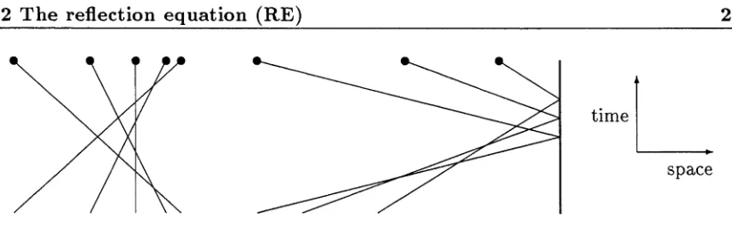
The reflection equation (also called the boundary Yang-baxter equation) had its origin in Cherednik’s (1984) work in factorizable scattering 5-matrix theory on a half line [25]. In this scenario the multi-component 5-m atrix factorises into a product of 2-particle 5- matrices k™S as well as particle-wall 5-matrices kT describing the interactions of elastic particle collisions with a wall. The multi-component 5-matrix with and without the presence of a boundary is illustrated in figure 2.2.
2.2 T h e r e flec tio n e q u a t io n ( R E ) 23
time
[image:30.526.63.473.47.175.2] [image:30.526.137.393.380.587.2]space
Figure 2 .2 : M ulti-com ponent S-m atrix for norm al scattering (left) and for scatterin g on a half line (right)
The conditions for this factorisation are (disregarding the conditions involving kT (0))
l_2S(u) J.35 (u + v) f S ( v ) = 23S(«) l_35(ti + (2.3)
2T (u)0*5(2« + v)IT( u + v) +25(«) = i ‘S(w) v) + v) ) (2.4)
where e = + , —,0 labels the 2-particle S-matrix for a reflected, unreflected, reflected- unreflected pair of particles respectively. Pictorially, the factorisation condition (2.3) is represented by figure 1.6 and analogously the representation of factorisation condition
(2.4) is given by figure 2.3.
Figure 2 .3 : B oundary factorisation condition for scattering theory on a half-line
Sklyanin (1988) later formulated this theory in the framework of open quantum spin chains using operator algebraic language traditional to QISM [80]. However he goes on to write:
24 T h e R e fle c tio n E q u a tio n an d D o u b le R o w T ra n sfer M a tr ix
In fact the formulation quite easily extends also to the face language through the correspon dence given on page 17 as well as face-vertex boundary intertwiners yet to be discussed.
The formulation of Sklyanin involves the introduction of algebras T_ and 7+ defined by a given R-matrix and the relations
#1 2(^1 2) T -(« i) #1 2(^1 2) 7 - (u2) = 7 - { u 2)Ri2{u^2) 7-{ui) R l2{ul2) (2.5)
and
Rn(ül2) O+Mlil) Rl2(üi2
-
2v)
7+2{u2) ^ = 7+2[u2)R\2(ü+2 - 2?7) 7 + 1 (ui) R n ( ü i2)where t{ is the transposition operation in End(V^). The subscripts in R xy and s u it
perscripts x in “J± refer to the actions on Vx0 Vy and Vx, respectively. The constant 77
characterises the R-matrix so th at
R \ \ {u) R U -u - 2r/) = p{u) (2.7)
where p(u) is some scalar function. Along with the crossing unitarity (2.7) and symmetry condition R \ 2(u) = R[22(u) , commutativity of the quantities t(u) follows
[*(ui),t(u2)] = 0 Vwi,w2 (2.8)
where
t(u) = tr 7+{u) 7-{u) (2.9)
T h e d o u b le row tr a n sfe r m a tr ix (D R T M )
In vertex and face terminology these t(u) correspond to double row transfer matrices with 7 ± corresponding to the left (+) and right ( —) half in the pictorial representation
(2.10). The trace connects these two halves (as indicated by the dotted lines).
(2.10)
The vertices represent the R-matrices (the details of spectral parameter location is dis cussed later) and we have two new objects which are called R-matrices K± (u) (corre sponding to the T(u) of Cherednik in (2.4)) or commonly boundary Boltzmann weights. All the internal edges are summed.
i<+0
M =
24
K - ß M =
2.2 T h e r e f l e c t i o n e q u a t i o n ( R E ) 25
In the face language the corresponding boundary weights are represented as
a a
( a \
\
( a \
/
I<i b u
=
u y b Kr
b u = b \ U\ c
/
/ \ c/
\
c c (2.12)
where b — a — a and b — c — ß for the alternating DRTM. So far the structural composition of the DRTM has been discussed without going into the details of the orientations of the composing bulk and boundary weights, i.e., in which corners the spectral parameters lie in the vertex representation, correspondingly, in which corner the ‘ta g ’ lies in the face representation. This is for the reason th at there are two main ways of fixing the orientations. Let us first fix the symbolic notation
(2 .1 3 )
[image:32.526.134.407.407.468.2]following the notation given in figure 1.4. The two ways of defining the DRTM are called here the homogenously oriented DRTM and the alternatingly oriented DRTM, both shown in figure 2.4. (Remembering that the dotted lines identify two edges as if they were the same edge and all internal heights are summed.)
Figure 2.4: Homogenous (left) and alternating (right) structures of the DRTM.
Getting back to DRTM commutativity, the proof of (2.8) given by Sklyanin is purely algebraic. Diagramatical representations of this proof were given in [19] for the face models using a homogenous DRTM. It turns out th at this definition of the DRTM does not allow diagonal solutions for the boundary weights in general. However the alternating DRTM by its very nature always allows for the possibility of diagonal weights.
Here is given a constructive proof of commutativity using alternating DRTMs. It is an alterrative approach to the usual method, not following Sklyanin’s algebraic proof directly.
C om m u ta tion o f th e altern a tin g D R T M s for a face m od el
Oir aim is to commute two alternating DRTMs and to this end the strategy is to build up the ways of commuting two single row transfer matrices in all possible orientations.
26 T h e R e f le c t io n E q u a t io n a n d D o u b le R o w T r a n s fe r M a t r ix
With inversion (see page 20) this is enough to ensure commutation of face row transfer matrices for periodic boundary conditions, as in the vertex case. The following three relations are also satisfied
where u' = A — u, v' = A — v and
a a
c c
(2.15)
(2.16)
(2.17)
(2.18)
The first two, (2.15) and (2.16), follow directly from (1.38) by adjusting spectral param eters and rotation through tt/ 3. The less trivial (2.17) is a consequence of the inversion relation (2.19) which follows easily from (1.44) in the case of the bulk weights satisfying crossing symmetry
(2.19)
Now consider the problem of finding an operation E that acts on an ordered list of 4 symbols such th at E(a, a\ 6 , b') = (6 , 6', a, a')E. It is easy to decompose E into a product of elementary permutation operators ezj which interchange the i-th and j-th symbol in an ordered list. The shortest of these decompositions is equivalent to E = 623612634623.
Identifying these e*j with the intertwining bulk weights above, (2.14-2.17), and the symbols with orientations of row transfer matrices, we find the following ‘fused’ inversion
2.2 T h e reflection eq u ation (R E ) 27
where g(u,v) = Q\(u — v')Q2(u + v — A). These equations, (2.20-2.21), already define an integrable face model with periodic boundaries. They also lead easily to an integrable face model with open boundaries as will now be demonstrated by showing that the associated DRTMs commute.
Step 1. Start with T(u) T(v)
28 T h e R e fle c tio n E q u a tio n an d D o u b le R o w T ra n sfer M a tr ix
Step 3. Use ‘fused1 YBE to horizontally zip through exchanging the weights of T(u) and 7 »
Step 4. Thus commutation occurs if the following equations are satisfied
Step 5. Using inversion (to cancel the g(u,v)) and setting f ( u , v) = 1, one can put these equations into a more symmetric form called the reflection equations:
Under appropriate relabelling and using the face-vertex correspondence these equations become equivalent to Sklyanin’s equations (2.6) and Cherednik’s factorising condition (2.4) for the equation on the right.
2.3 P r o p e r tie s o f t h e R E a n d s o lu tio n s 29
2.3
P r o p e r tie s o f th e R E an d s o lu tio n s
Following in the footsteps of Sklyanin who found various isomorphisms between the alge bras T -and (which represent right or left halves of the DRTM as distinct from just the boundary P-matrices) we find the following relationships between left and right solutions to the REs. Firstly define
a " a
(2.22)
similarly to (2.18). The left reflection equation then becomes
(2.23)
after reparameterising u —»■u' =■ A — u and v —>• v' = A — v. Since the ‘tags’ take care of orientations we are free to rotate this entire equation upside down from which it immediately follows that
a a
c c
is a solution of the left RE. (It may be noted th at this is reminiscent of the crossing symmetry for bulk weights.) This allows one to concentrate on solving only the right RE. This relationship reduces to that of Sklyanin’s isomorphism X : 9"_—>■ “J+ in the vertex limit
A -{7-W } = 7 i ( - u - » ) ) (2.25)
Skyanin’s approach for constructing open integrable spin chains was extended by Mez- incescu and Nepomechie to include non-symmetric R-matrices which are only PT-invariant [71]. This formulism was used to construct a large class of integrable models which have quantum algebra invariance [69, 70].
30 T h e R e fle c tio n E q u a tio n an d D o u b le R ow T r a n sfe r M a tr ix
S o lu t io n s o f t h e R E
The formulisation given above allows one to construct a model with open boundaries given an integrable model with periodic boundaries. While some a attem pts have been made to find a standard procedure for finding the boundary weights given the bulk weights, most of the solutions found have been through directly solving the RE. These are sum marised in the following table, which is by no means exhaustive.