Modelling decadal secular variation with only magnetic diffusion

Advance Access publication 2019 February 17

GJI Geomagnetism, rock magnetism and paleomagnetism

Modelling decadal secular variation with only magnetic diffusion

Maurits C. Metman,

Philip W. Livermore ,

Jonathan E. Mound

and Ciar´an D. Beggan

1_{School of Earth and Environment, University of Leeds, Leeds LS2 9JT, United Kingdom. E-mail:[email protected]} 2_{British Geological Survey, Edinburgh EH14 4AP, United Kingdom}

Accepted 2019 February 15. Received 2019 February 13; in original form 2018 November 22

S U M M A R Y

Secular variation (SV) of Earth’s internal magnetic field is the sum of two contributions, one resulting from core fluid flow and the other from magnetic diffusion. Based on the millenial diffusive timescale of global-scale structures, magnetic diffusion is widely perceived to be too weak to significantly contribute to decadal SV, and indeed is entirely neglected in the commonly adopted end-member of frozen-flux. Such an argument however lacks consideration of radially fine-scaled magnetic structures in the outermost part of the liquid core, whose diffusive timescale is much shorter. Here we consider the opposite end-member model to frozen flux, that of purely diffusive evolution associated with the total absence of fluid flow. Our work is based on a variational formulation, where we seek an optimized full-sphere initial magnetic field structure whose diffusive evolution best fits, over various time windows, a time-dependent magnetic field model. We present models that are regularized based on their magnetic energy, and consider how well they can fit the COV-OBS.x1 ensemble mean using a global error bound based on the standard deviation of the ensemble. With these regularized models, over time periods of up to 30 yr, it is possible to fit COV-OBS.x1 within one standard deviation at all times. For time windows up to 102 yr we show that our models can fit COV-OBS.x1 when adopting a time-averaged global uncertainty. Our modelling is sensitive only to magnetic structures in approximately the top 10 per cent of the liquid core, and show an increased surface area of reversed flux at depth. The diffusive models recover fundamental characteristics of field evolution including the historical westward drift, the recent acceleration of the North Magnetic Pole and reversed-flux emergence. Based on a global time-averaged residual, our diffusive models fit the evolution of the geomagnetic field comparably, and sometimes better than, frozen-flux models within short time windows.

Key words: Dynamo: theories and simulations; Electromagnetic theory; Magnetic field vari-ations through time; Inverse theory; Numerical approximvari-ations and analysis.

1 I N T R O D U C T I O N

The magnetic field generated within the Earth’s fluid outer core exhibits continuous change in time over yearly to decadal timescales, termed secular variation (SV). Global geomagnetic field models constructed from ground-based observatories, satellites and other data sources are often expressed in terms of time-dependent Gauss coefficients{gm

l ,h m

l }, each of degreeland orderm, which correspond to a spherical harmonic partitioning of the field; decadal changes of selected spherical harmonic components are shown in Fig.1.

SV results from two processes within the liquid core: interaction between outer core fluid flow and the magnetic field and magnetic diffusion (e.g. Jackson & Finlay2015). The general balance between these two processes is quantified by the magnetic Reynolds number

Rm= UL

η =

τd

τu

, (1)

withU and Lcharacteristic fluid velocity and magnetic length scales, respectively,ηthe magnetic diffusivity and typical timescales for diffusion and advection denoted byτdandτu, respectively. Estimates of these quantities (L=103km,U=20 km yr−1andη=63 km2yr−1, e.g. Jackson & Finlay2015) yield the timescalesτd=16 kyr andτu=65 yr andRm∼102(where the tilde denotes order of magnitude). The disparity between these timescales implies that for decadal SV diffusion may be neglected, an approximation commonly referred to as that of frozen flux as introduced by Roberts & Scott (1965).

S58 CThe Author(s) 2019. Published by Oxford University Press on behalf of The Royal Astronomical Society.

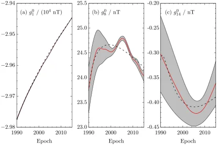
Figure 1.Time-series of the Gauss coefficientsg0

1 (a),g08 (b) andg014(c) obtained from the mean COV-OBS.x1 field model for the period 1840.0-2015.0 (Gilletet al.2015a).

This assertion has proven extremely valuable over the past decades. Not only have several authors demonstrated a mathematical consistency between geomagnetic observations and frozen-flux constraints on core field evolution (e.g. Gubbins1984; Constableet al.1993; Wardinski & Lesur2012), the approximation has also allowed the inversion of SV observations on the Earth’s surface and above for core fluid motions along the core–mantle boundary (CMB; e.g. Vestineet al.1967; Whaler1980; Bloxham1988). In addition, frozen flux has been utilized to further constrain the space and time-variability of core fluid flow (Olsen & Mandea2008; Aubert2012; Livermoreet al.2017), to forecast SV over periods of less than a decade (Beggan & Whaler2009; Whaler & Beggan2015; B¨arenzunget al.2018; Beggan & Whaler 2018) and to explain length-of-day variations resulting from core–mantle coupling (Jaultet al.1988; Jacksonet al.1993; Gilletet al.2015b). Although frozen flux has been shown to be a useful approximation, there is ongoing discussion regarding what part of the observed SV can truly be attributed to magnetic diffusion, which relates to the parameters that defineRm(eq.1). First, typical estimates forLare based only on horizontal CMB field morphology, and a typical magnetic length scale in the radial direction remains poorly constrained (e.g. Holme 2015), although for the region just below the CMB it has been estimated at several tens to hundreds of km (Amit & Christensen2008; Chulliat & Olsen2010; Terra-Novaet al.2016). In light of this, several authors have stressed the inevitable failure of the approximation if magnetic features are indeed of sufficiently small radial scale, for example, due to the concentration of toroidal field beneath the CMB through fluid upwelling, a process known as flux expulsion (Bloxham1986; Gubbins & Kelly1996). Second, the velocity scaleUis usually estimated by directly attributing the observed secular westward drift of equatorial magnetic features (Halley1692; Finlay & Jackson2003) to fluid flow, showing only (in a circular argument) that the frozen-flux approximation is consistent with highRm. What this argument does not consider, however, are alternative processes that may explain the westward drift [such as waves (Hide1966) or diffusion] that would require smaller magnitude flows to explain the residual SV and thus have a smaller associatedRm.

Aside from these theoretical considerations, the importance of diffusion has also been highlighted with numerical simulations of the geodynamo. Such models can yield observable diffusion through flux expulsion (Aubertet al.2008; Aubert2014), despite the fact that these models are typically characterized by Earth-likeRm(Christensenet al.2010). Furthermore, the special geodynamo case of steady core fluid motion has been demonstrated to be incompatible with frozen flux (Gubbins & Kelly1996; Love1999). More recently, Barrois

et al.(2017) employed statistics derived from geodynamo simulations to demonstrate that even on short timescales diffusion contributes up to approximately 10 per cent of the overall SV at the CMB, although separating this diffusive signal from errors related to finite horizontal resolution remains non-trivial (Barroiset al.2018).

Local failure of frozen flux has also been inferred from observations of the core magnetic field, using the constraint that without diffusion the total magnetic flux through patches bounded by null-flux curves should remain steady (Backus & Bullard1968). For instance, recent rapid change of the North Magnetic Pole (NMP) and of the radial magnetic field under St. Helena have been attributed to flux expulsion (Chulliatet al.2010; Chulliat & Olsen2010). Gubbins (1996) made an initial attempt to invert for core motion with the explicit inclusion of diffusion and estimated a considerable radial gradient of toroidal field of 20 nT m−1_{beneath the South Atlantic, sufficient to explain the} local intensification of magnetic flux of 500 MWb. However, it remains difficult to unambiguously detect such expulsion patches and hence a

signature of magnetic diffusion in the core (Amit2014). Furthermore, it is challenging to distinguish magnetic diffusion from energy transfer between unresolved small-scale flow and the observed large-scale magnetic field (Roberts & Glatzmaier2000).

In this paper, we will test whether magnetic diffusion is capable of generating decadal SV that matches the observation-based model COV-OBS.x1 (Gilletet al.2015a). To do this, we use a variational formulation, where we seek the 3-D structure of an initial magnetic field whose subsequent evolution best explains SV over a defined time window. Variational data assimilation has been implemented successfully in several nonlinear geodynamo models (Fournieret al.2007; Liet al.2014) but here, owing to the lack of any coupling through the absent flow, the optimal initial field can be found in a particularly simple way as a solution to a linear system. We consider various time windows to assess whether a purely diffusive model is consistent with SV on yearly, decadal and centennial timescales. This approach allows us to explore a new end-member model of the SV, that of pure diffusion, and compare it against models of the more traditional frozen-flux type. Our purely diffusive model is not intended to fully represent the mechanism responsible for SV, but rather to test whether it is sufficient to reconstruct the observed SV and to probe the field below the CMB using the inherent assumptions of the model. While the formalism by Gubbins (1996) permits diffusion as a correction term for frozen flux and could be utilized to jointly invert observed field evolution for the frozen-flux and diffusive contributions to SV, we present here a new scheme that considers diffusion as the sole contribution to SV.

This work is structured as follows: we first describe in Section 2 how we optimize the initial full-sphere magnetic field to match SV through its diffusive evolution; the resultant diffusive models along with their general and local characteristics are presented in Section 3; Section 4 discusses the geophysical implications of our results. Four appendices describe technical details including depth-sensitivity and numerical convergence.

2 M E T H O D S

In this section we present our variational formalism for a diffusing 3-D magnetic field. Assuming that the solid inner core has the same electrical conductivity as the liquid core, the same diffusion equation is obeyed everywhere in the core by the magnetic field and we therefore seek full-sphere solutions, which are also therefore valid in a spherical shell. We begin by briefly introducing the associated forward problem and its canonical solutions: the decay modes. These functions are used in Appendix A to determine the resolving power of our methodology as a function of depth. We also present an alternative representation of the forward model using Galerkin polynomials, which turns out to be numerically much better conditioned than that based on decay modes. Finally, we consider a means of regularizing the inverse solution by penalizing the total magnetic energy.

2.1 Decay modes

Here, a set of analytical (forward) solutions to the (dimensional) magnetic diffusion equation are given (Gubbins & Roberts1987). If we were provided with the structure of the magnetic field throughout the entire core, these solutions would describe the temporal evolution of that field in the absence of fluid flow. We start with the 3-D magnetic diffusion equation for uniform magnetic diffusivity, which reads

_∂

∂t −η∇2

B=0, (2)

wheretis time andBdenotes the core field. Because the field is solenoidal, it may be partitioned into its toroidal and poloidal parts:

B=BT+BS= ∇ ×(Tr)+ ∇ × ∇ ×(Sr), (3)

withBT andBSthe toroidal and poloidal field, respectively, andTandStheir respective defining potentials. Applying this decomposition simplifies the diffusion problem to the scalar equations

_∂

∂t −η∇

2

T =

_∂

∂t −η∇

2

S=0. (4)

Both of these equations may be solved to obtain a diffusive description for all vector components of the field. However, the toroidal field inside the core is unobservable (the field outside the core is purely poloidal) and we therefore restrict attention to the poloidal diffusion problem by settingT=0. The scalarSis then expanded in real-valued Schmidt quasi-normalized spherical harmonicsYα(θ,φ) (θandφdenote colatitude and longitude, respectively), the indexαcorresponding to the harmonic of degree 1≤l_α≤Lfor someLand order 0≤m_α≤l_α, which has either azimuthal sine or cosine dependence. This representation then requires

_∂

∂t −ηDl2α

r s_α(r,t)=0, (5)

withrradius,s_αthe spherical harmonic coefficients ofSand where we have defined the operator

D2_lαf(r)= _∂2

∂r2 −

l_α(l_α+1)

r2

f(r). (6)

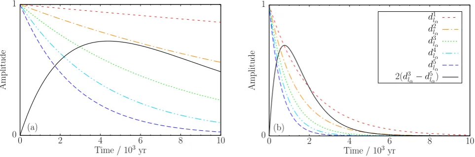
Figure 2.Time dependence of the first five decay modesdn

l_αfor (a)lα=1 and (b)lα=14, normalized to have initial positive unit amplitude. While a single mode always decays monotonically, a linear combination of these functions may exhibit transient strengthening (solid curve).

This equation has the solution

s_α(r,t)= N

n=1

qn αdln_α(r,t),

= N

n=1

qn αjlα

kn lαr

c exp −η kn lα c 2 (t−t0)

, (7)

wheredn

lα(r,t) denotes thenth decay mode of degreelα, theq n

αa set of constants, jlα(z) the spherical Bessel function of the first kind,klnα the

nth root of jlα+1(z) andcthe core radius. The initial state is given by the expression evaluated at the initial timet0. The decay modes form an orthogonal set in terms of an all-space energy norm (Backus1958). This solution allows us to express the radial fieldBrup to degreeL satisfying the diffusion equation as

Br(r,t)= 1

r

L(L+2) α=1

l_α(l_α+1)s_α(r,t)Y_α(θ, φ),

= 1

r

L(L+2) α=1

N

n=1

qn

αlα(lα+1)jl_α

kn l_αr

c exp −η kn l_α c 2 (t−t0)

Y_α(θ, φ). (8)

Using this decay mode expansion, we may already describe our following inverse approach qualitatively. Consider, for example, Fig.2 showing the time dependence of the first five modes forlα=1 (a) andlα=14 (b), where their initial amplitude has been normalized to unity. It can readily be seen that all individual modes decay monotonically with time, and that their respective rate of decay increases withl_αandn. However, a linear combination of modes need not always decay, as is the case for the differenced3

l_α−d 5

l_α(solid black curve), which exhibits transient growth (e.g. Livermore & Jackson2006). Although the modes are formally orthogonal in a global sense, they are not orthogonal when evaluated at a single value ofr=cand thus transient effects can readily occur. In the same way, there may exist a combination of modes that describes an initial field configuration whose evolution matches the observed SV (which shows in general both transient decay and growth) over some time window.

We also use the decay modes a priorito estimate the sensitivity of the CMB field evolution to magnetic diffusion within different regions of the core. It may be expected that the core is not sampled uniformly; we consider diffusion only over time intervals of decades to centuries, and bearing in mind the slow 16 kyr timescale of global modes, the diffusive evolution of deep magnetic structures may not have a signature in the CMB SV within such time intervals. In Appendix A, we show that for pure diffusion the CMB field evolution can only constrain the magnetic structure within a region close to the CMB. This layer spans approximately the top 80 km when one decade of diffusion is considered (Fig.A2a); for 175 yr, which matches the full COV-OBS.x1 time window, this region extends to roughly the upper 400 km (Fig.A2b). Therefore, even though we shall seek an optimal full-sphere magnetic structure, structures below the sensitivity depth should not be interpreted geophysically.

2.2 A Galerkin discretization

While the decay modes solve the magnetic diffusion equation exactly, the series in eq. (8) is characterized by slow (algebraic) convergence inN(e.g. Boyd2000), associated with poor numerical conditioning of the inverse problem. In the following, as an expedient alternative, we solve the radial diffusion problem (eq.5) with a Galerkin polynomial basis set in radius, yielding faster (spectral) convergence and much

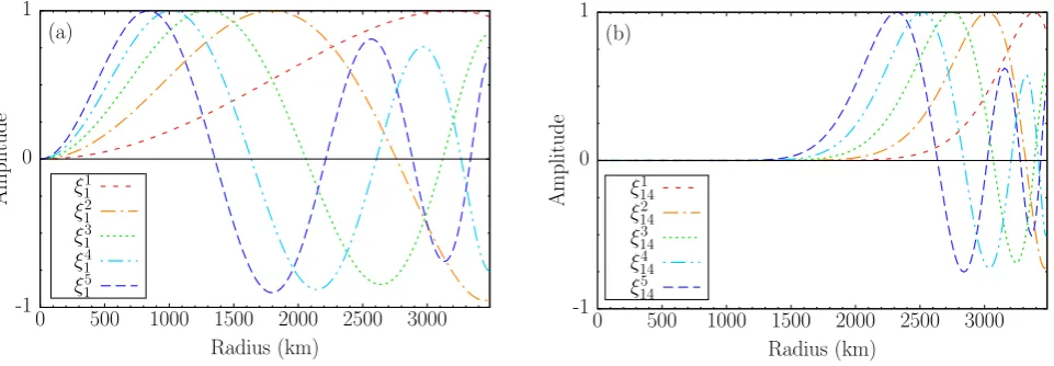
Figure 3. The Jacobi polynomialsξ_ln_α as a function of radius, forlα=1 (a) andlα=14 (b), here normalized such that their extremum is of positive unit amplitude.

better conditioning. To do so, we approximate

r sα(r,t)= N

n=1

ξn

α(r)ϕαn(t)qαn, (9)

withϕn

α(0)=1. We choose the radially dependent basis functions to be built from weighted Jacobi polynomials (Livermore2010) of the form

ξn

α(r)= Anαψαn(r/c), (10)

whereAn

αis a normalization constant and

ψn

α(r)=rlα+1

n(2l+2n−1)P(0,lα+1/2) n (2r

2₋

1)−(n+1)(2l+2n+1)Pn(0−,l1α+1/2)(2r 2₋

1)

, (11)

with P(α,β)

n (z) a Jacobi polynomial. The poloidal vector modesBnα= ∇ × ∇ ×(ξαnYαrˆ) have the property of orthogonality over all space (Chenet al.2018; Liet al.2018) through the integral (see also Appendix D)

R3

Bn_α·B_βpdV = 4πlα(lα+1)

2l_α+1 c 0 ∂ξn α ∂r _∂ξp β ∂r

+lα(lα+1)

r2 ξ

n αξβpdr+

l_α cξ

n α(c)ξβp(c)

, (12)

:= ξn α, ξ

p

βlα, (13)

which may be used to find the constantAn

α. Such orthogonality is identical to that satisfied by the decay modes, but the Galerkin modes are much better numerically conditioned as they show asymptotic spectral convergence. The radial dependence of these functions is visualized in Fig.3, which are not only regular at the origin, but also obey the matching conditions appropriate to an external potential field.

Through substitution of the approximation (eq.9) in the radial diffusion equation (eq.5), and by projecting the result onξj

α(r) using eq. (), we obtain the system of equations:

∂

∂tϕα=ηHαϕα, (14)

whereϕ_α:=(ϕ1

α, ϕα2, . . . , ϕαN)Tis the time-dependent solution for a givenαandHα,i j := D2l_α[ξαi], ξαjlα. The total solution, exact within the truncation specified, can be written

r s_α(r,t)=ξ_αT(r)expmηH_α(t−t0) qα, (15)

where expm[·] denotes the matrix exponential. Whent=t0, the given matrix exponential is the identity matrix, in which case one recovers the initial magnetic structure. Note also that for the particular case of using the decay modes in place of the Galerkin polynomials, the matrix H_αand so expm[H_α] are diagonal, and so the above representation is equivalent to the solution given in eq. (7).

2.3 Unregularized inverse strategy

2.3.1 A least-squares variational analysis

With this discretization of the diffusive forward problem, we are now in a position to define the variational scheme. Accordingly, we consider the objective function

Runreg=

T

CMB

Bobs

r (t)−Bˆr(t) 2

dSdt, (16)

where the time period isT=[t0,te],Brobsis the radial field prescribed by a time-dependent geomagnetic field model, and ˆBr(t) denotes the radial component of our modelled field. We seek an initial structure of the magnetic field that minimizesRunreg.

Discretizing the temporal integrals and expressingRunregin terms of the model coefficients gives the reduced form

Runreg=(g−Dqˆ)TW(g−Dqˆ), (17)

withgandˆqvectors containing all Gauss coefficients (which are known) evaluated at a set of time points and all model coefficients (which are to be found), respectively, the matrixDa blockwise-diagonal (one block per spherical harmonic mode) forward mapping describing purely diffusive SV, andWa diagonal weighting matrix related to the scheme of numerical time integration. Adopting decay modes in place of Galerkin polynomials results in a comparable form but with differentD. For the derivation and exact definition of these quantities, the reader is referred to Appendix B. Key here is the fact that the objective function depends only quadratically onˆq, in contrast to much more complex schemes that include nonlinear feedback from the core flow (e.g. Liet al.2014). Taking variations to find the minimum ofRunreg, with respect to ˆq, then directly gives the optimal set of coefficients

ˆ

q=(DTWD)−1

DTWg. (18)

In this paper we will consider only using this variational technique with the geomagnetic field model given by the mean of the COV-OBS.x1 ensemble (Gilletet al.2015a). This model of spherical harmonic degreeL=14 spans 175yr (1840.0–2015.0) that is sufficient to cover our range of time window lengths and extends (almost) to the present day using modern satellite data.

It is worthwhile briefly considering our inversion scheme in the landscape of other mathematical inverse problems associated with diffusion. A well-known example is the backwards heat conduction problem (e.g. Miranker1961) in which complete knowledge of a temperature profile is assumed at some final timet=te, and the task is to find the initial temperature profile att=t0that evolves through heat diffusion (conduction) to match the final state; such a problem is, in general, tractable but ill-posed. The problem that we consider here is quite different: as described above, the structure of the evolving magnetic field is known only atr=c(rather than everywhere), but for all times in [t0,te] (rather than at a single time). We have therefore traded complete information of structure at a single time for partial structural information at all times. A solution of the backwards conduction problem requires two boundary conditions, as it is a second-order equation like the magnetic diffusion equation. In our case we also supply two sets of information at the boundary. First we constrain the poloidal scalar through matching to the field model. Second, we constrain the radial derivative of the poloidal scalar by virtue of the matching condition associated with the electrically insulating mantle atr=c. Our problem is therefore fully specified and optimal solutions exist, although we may not be able to fit the data exactly (Runreg>0, see e.g. Appendix C).

2.3.2 Matrix conditioning and choice of radial basis functions

In order for our inverse approach to be viable, it is necessary that the solution of eq. (18) is numerically realizable. Of particular concern is whether the numerical inverse of the weighted Gramian matrixDT_{WDis computationally tractable, which can be quantified by its condition} number. As an approximate rule of thumb, ifDT_{WDhas a condition number 10}a_{, the number of inaccurate trailing digits of ˆqisawhen the} solution is expressed numerically with floating-point representation. Thus in standard double-precision (about 16 digits), with a condition number of 1012_{, ˆqcan be expected correct to about four significant figures; matrices with condition numbers in excess of 10}16_{or so cannot} be inverted in double precision.

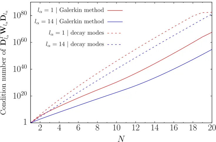
Fig.4shows the condition numbers (measured in the standard 2-norm) for the diagonal blocks ofDassociated withlα=1 andlα=14, representing the extreme cases, as a function of the number of basis functions (either polynomial or decay modes). Here, we used 201 time points (this ensures a numerically converged solution, see Appendix C), and sextuple (256-digit) precision in place of the more commonly used double (16-digit) precision to ensure that all calculations shown were accurate. The condition numbers, many of which are far in excess of 1016_{, highlight the ill-posedness of the inverse problem. Physically, this may be understood by the difficulty of constraining the magnitude} of initially fine scales because they diffuse very rapidly: this is a problem for both the decay mode and Jacobi polynomial representations. In practice, the large condition numbers mean that in double precision the radial resolution available for this method is extremely limited.

However, there are two ways in which we can mitigate these effects. First, it should be noted that the Galerkin scheme has a much lower condition number than the decay modes for fixedN, an effect particularly notable for block matrices of high spherical harmonic degree. This means that for any given condition number threshold the Galerkin method allows more radial modes and therefore increased resolution. The better conditioning achieved with the Galerkin method therefore motivates us to apply it to our inverse approach. Second, we can use very

Figure 4. The condition number of the weighted Gramian block matrices, forlα=1 (red) andlα=14 (blue), as a function ofN, the number of basis functions used and using either decay modes (dashed) or the Galerkin polynomials (solid).

high precision in our calculations (we have used up to 256 digits using the symbolic toolbox for Matlab), making possible a resolution of 30 radial polynomial modes (with typical condition numbers of 1095_{and 10}70_{for the decay modes and Galerkin polynomials, respectively).}

2.4 Regularized inverse strategy

2.4.1 A penalized variational approach

Minimizing an objective function of the form ofRunreg(eq.16) ensures an optimal fit to SV without consideration of the spatial complexity of the initial optimal magnetic field. It may therefore be unsurprising that the initial (t=t0) magnetic structures can show large spatial fluctuations in amplitude. For example, if we consider the optimization over the time window 2005.0-2015.0, the associated initial field over the upper 80 km of the core (its sensitivity depth: the field below this depth is likely poorly resolved, see Appendix A), we find a root-mean-square (RMS) average|B|of about 1025_{mT. Similarly, for the period 1840.0-2015.0, the optimal model has an RMS field strength in excess of} 1029_{mT over its sensitivity depth of 400 km. Such huge amplitudes cannot be reconciled with the RMS field strength for the core, which} has been estimated at 2.5 to 4 mT (Buffett2010; Gilletet al.2010). It is likely that the ill-posedness of the unregularized inverse diffusion problem leads to these extreme solutions.

Therefore, we consider also the minimization of an associated regularized objective function

Rreg=

T

CMB

(Brobs−Bˆr)2dSdt+λ

R3

ˆ

B20dV, (19)

where the second term corresponds to penalizing the energy of the initial magnetic field ˆB0over all space, scaled with a damping parameter

λ. Note that for purely diffusive SV the total magnetic energy monotonically decays with time (e.g. Gubbins & Roberts1987) and this regularization term will therefore penalize magnetic energy over the entire time period. Nevertheless, this constraint still permits any local exchange of magnetic energy, such as the overall energetic growth at the CMB observed for the 20th century (Huguetet al.2018). The choice of this regularization differs from that adopted elsewhere, for example, the dissipation norm of Gubbins & Bloxham (1985) and is motivated here by the very simple structure (see Appendix D for a derivation):

R3

ˆ B20=qˆ

T_ˆ

q. (20)

The discretized regularized objective function is then

Rreg=(g−Dqˆ)TW(g−Dqˆ)+λqˆTqˆ, (21)

whose minimum with respect to ˆqthen yields

ˆ

q=(DTWD+λIN L(L+2))−1DTWg, (22)

whereIpis thep×pidentity matrix, withp=NL(L+2).

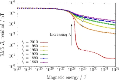
Figure 5.The RMS residual ofBras a function of the initial magnetic energy of the solution for several time windows (fromt0to 2015.0). Every datum represents a choice for the damping parameterλ. The diamonds indicate our preferred trade-off between the residual and regularization term.

2.4.2 Choosing the damping parameter

The solutions (eq.22) parametrize a 1-D family of solutions that minimize the associated objective functionRreg. We now address which solution we should choose. Ultimately, we are interested only in the solution that best describes SV with realistic amplitudes in the modelled core magnetic structure. In the following, we shall find values for this parameter we consider optimal based on howλaffects the trade-off between the residual and the regularization term.

Fig.5shows a trade-off curve forλshowing the RMS residual inBr[i.e. the square root ofRunreg(eq.16) averaged over the CMB and

T] as a function of the associated initial magnetic energy (defined over all space) for various time windows, where every datum represents a choice ofλ. These models have been calculated using double (16-digit) precision, 30 basis functions and 201 time points (these values ensure a numerically converged solution, see Appendix C). We note that for the data plotted, the regularization term ensures that double-precision is sufficient: clearly asλ→0 (and in fact for values of the energy in excess of roughly 1032_{J) we recover approximately the unregularized} problem for which much higher precision is needed. For all time windows, there appears to exist a regime in which the solutions do not contain enough energy to allow an adequate fit to the observations, typically when the energy is below 1027_{J. Decreasingλand so increasing the} energy beyond this point to roughly 1029_{J, yields a significant reduction in the residual. This is particularly notable for short time windows;} allowing increased energy in the longer time windows results in a relatively low improvement in the residual.

For all time windows, we considerλoptimal if it is on the ‘knee’ of the trade-off curve after the initially rapid decline of the residual (diamonds in Fig.5). This knee is difficult to define quantitatively for time windows spanning several decades; therefore, all preferred values forλhave been picked by eye, which range between 10−18_{and 10}−3_{(Supporting Information data file 1 lists these values). Lastly, we note} that all our preferred models have a full-core RMS field strength between 0.6 and 1.3 mT and are therefore consistent with the 2.5 or 4 mT estimates provided by Gilletet al.(2010) and Buffett (2010).

3 O P T I M I Z E D P U R E LY D I F F U S I V E M O D E L S

3.1 Regularized models

Here we present a set of purely diffusive models comprising regularized inversions for an initial magnetic structure whose subsequent evolution is described by the mean COV-OBS.x1 model. These solutions have been obtained for varying time windows terminating at 2015.0 and have been computed with 30 basis functions, 201 time points (ensuring a numerically converged solution, Appendix C) and optimalλ values that have been selected using the criteria presented in Section 2.4. For these models, we show a number of results. First, we compare time-series of selected Gauss coefficients over a single time window. Second, we presentBrresidual error spectra for several time windows.

Figure 6.Comparison between time-series of selected Gauss coefficients from the regularized diffusion model for 1990.0-2015.0 (black dashed) and the mean COV-OBS.x1 model (solid red). Grey shaded areas represent the mean COV-OBS.x1 model±one standard deviation.

We also demonstrate how the total residual changes as a function of the window length. Finally, we mapBrand ˙Brresiduals at the CMB and at selected epochs.

Fig.6shows time-series of the Gauss coefficientsg0

1,g80andg140, for the period 1990.0-2015.0 from the COV-OBS.x1 mean (solid red) and diffusive models (dashed black). The grey shaded areas correspond to the time-dependent one standard deviation error bounds. Despite the correct qualitative behaviour of the diffusive model, only the high-degree coefficients are fit within the COV-OBS.x1 uncertainty. For instance, while the regularized diffusion model captures the overall decay ofg0

1, the diffusive time-series is generally outside the COV-OBS.x1 error budget. Conversely, the regularized fit tog0

14is well within the COV-OBS.x1 error budget at all times. This effect is in part driven by the relative increase in the COV-OBS.x1 error budget with degree: for degree 1 the relative uncertainty is small, typically<0.1 per cent for this period, whereas for degree 14 it may be as large as 25 per cent. Nevertheless, the diffusive fits tog0

1andg 0

8also lack the short-term variability required to fit COV-OBS.x1 within the uncertainty at all times.

That diffusion captures higher degree features of the field more easily is quantified with spherical harmonic error spectra (Fig.7), which have been computed for various time windows using

E(l_α)= (lα+1) 2 2lα+1

a c

2lα+4 l_α

m_α=0 1

T

T

g_α(t)−gˆ_α(t)2dt. (23)

This spectrum relates to the residual in eq. (16): the sum ofE(l_α) overl_αis the mean squared error inBraveraged overTand the CMB. Shown as the solid curves in Fig.7are also the COV-OBS.x1 uncertainty spectra computed with eq. (23) and with the integrand taken to be the variance; the total mean squared uncertainty is then the sum of the uncertainty spectrum. Readily notable is the contrast of rather flat diffusion error spectra, and the COV-OBS.x1 uncertainty spectra increasing monotonically withlα, demonstrating that high-degree features are more likely to be fit within the uncertainty. Also, for all degrees, the average error increases when a longer time window is considered, therefore for longer periods only relatively high-degree features are captured well: for 2010.0-2015.0 degrees 3 to 14 are within the uncertainty bounds; for 1985.0-2015.0 only degrees 10 to 14 are within these bounds.

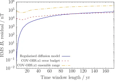
While for most degrees the regularized 1985.0-2015.0 error spectrum is orders of magnitude larger than the COV-OBS.x1 uncertainty, the total residual is actually smaller than the total uncertainty based on a single standard deviation. We confirm this by showing for the complete set of diffusion models the time-averaged RMS residual as a function of time window length, together with this uncertainty (Fig.8). It then becomes evident that with our regularized diffusion models, we may fit SV over 102 yr, without producing a time-averaged residual greater than the COV-OBS.x1 error budget based on one standard deviation. Additionally, we find 30 yr to be the longest time window for which regularized diffusion fits SV while the total residual is smaller than the total uncertainty at all points in time. Nevertheless, it is of note that if we consider the 1913.0-2015.0 (102 yr) diffusive model and compute the associated time-averaged residual over a shorter period

Figure 7.Time-averaged spectra of the residualBrat the CMB for the regularized diffusion models (dashed) and the time-dependent standard deviation of COV-OBS.x1 (solid). The line colours and symbols represent different time windows spanning fromt0to 2015.0.

Figure 8. The time average of the RMSBrresidual over the CMB as a function of time window length for the regularized diffusion models (solid blue). Also shown are two time-average global uncertainties for COV-OBS.x1, one computed with one standard deviation among Gauss coefficients (dashed red) and the other from maximum differences between the 100 published ensemble members and the ensemble mean (dot-dashed yellow).

(here taken as 1990.0-2015.0), we find it amounts to 4.78×104_{nT—now roughly 2.5 times as large as the total COV-OBS.x1 uncertainty} for the 1990.0-2015.0 period. A similar procedure but with these residuals evaluated at the Earth’s surface yields an average of 810.5 nT for the full period; when averaged over the 1990.0-2015.0 period with the use of the same model, this residual equals approximately 1162 nT. These differences are indicative of an overall temporal growth of the residual, which we find for almost any choice ofT. Shown in Fig.8 is also a more generous global uncertainty measure computed using eq. (23) based on the maximum difference between the 100 published COV-OBS.x1 ensemble members and the ensemble mean. It can be readily seen that the regularized diffusion models fit COV-OBS.x1 within this uncertainty bound over the full 1840.0-2015.0 period.

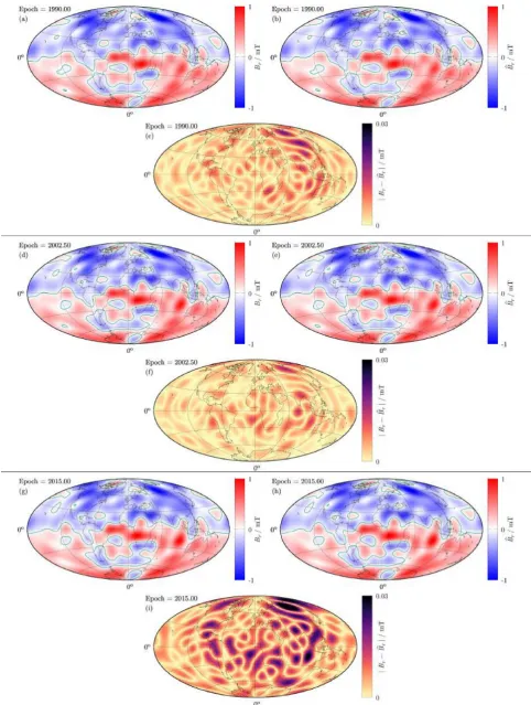
As the total error and its associated spectrum describe how well diffusion fits only in an average sense, we illustrate also how the residual varies spatiotemporarily. In Fig.9the radial field is shown at the CMB and at selected epochs, as prescribed by COV-OBS.x1 and the regularized 1990.0-2015.0 model (a,d,g and b,e,h respectively; see also animation S1, Supporting Information). Also shown at these epochs is the corresponding unsigned difference between these two models (Fig.9c, f and i; see also animation S2, Supporting Information). We find good global agreement between the models through visual comparison; this is also reflected by the associated error amplitudes, which are low compared to the radial field itself. Still, we observe an overall growth of the unsigned residuals with time, these errors being the largest towards the end of the period. Spatially, the residuals describe a pattern where the largest amplitudes reside in the Indo-Atlantic Hemisphere, in particular under Siberia, and the Pacific generally accommodating lower amplitudes. These high error amplitudes beneath the southern Indian Ocean and Asia correlate with regions for which significant secular acceleration has been reported (Olsen & Mandea2008). As such, Fig.9demonstrates that it is more difficult for the diffusion model to replicate COV-OBS.x1 where it locally describes relatively fast field change.

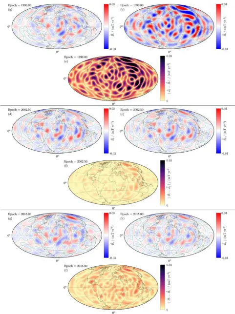
We confirm this statement by investigating the fit of SV on the CMB. Fig.10shows ˙Bron the CMB and at selected epochs for COV-OBS.x1 and the regularized 1990.0-2015.0 diffusion model (a, d, g, and b, e, h, respectively; see also animation S3, Supporting Information); the associated unsigned SV differences are given in c, f and i (see also animation S4, Supporting Information). The residual patterns in Fig.9bear resemblance to the SV described by COV-OBS.x1 as both are characterized by relatively large amplitudes under Siberia, the South Atlantic and the Indian Ocean, in particular at 2015.0. Furthermore, the residual SV amplitudes are relatively large compared to ˙Br, although it is of note that we do not explicitly minimize the SV residual. Particularly striking is the initially high amplitude SV described by the diffusion model, which is associated with large residuals at 1990.0. However, these amplitudes diminish quickly, and we find reasonable global agreement midway through the time period. The diffusion models tend to produce higher SV initially, which diminishes through time, such that they best explain the rate of change near the centre of the modelling period. The SV residuals increase in magnitude towards the end of the period, and by 2015.0 it is particularly difficult for the diffusion model to match the SV amplitudes beneath Siberia.

3.2 Comparison with core field characteristics and evolution

The results presented above, and in particular Fig.8, suggest that a globally optimized field structure with an associated diffusive time dependence is consistent with core field evolution on yearly to decadal timescales. In this section, we focus on how certain local features of the field are represented by these diffusive models.

3.2.1 Depth extent of reversed flux patches

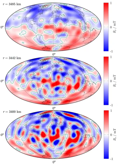
Fig.11shows the initial (t=t0) radial field for the regularized 1990.0-2015.0 diffusive model at selected depths inside the core (see also animation S5, Supporting Information). Because this model is expected to be poorly resolved below roughly 3400 km radius (see Appendix A), we only highlight the modelled field structure between this depth and the CMB. In general, the field is found to contain more structure and to be of higher amplitude at greater depth. Additionally, the axial dipole is less prevalent within deeper regions of the core, as reversed-flux patches (RFPs; Gubbins1987; Olson & Amit2006; Terra-Novaet al.2015; Metmanet al.2018), that is, areas horizontally bounded by null-flux curves where the sign ofBris opposite to the one expected from the dipole component of the field show a marked expansion and proliferation with increasing depth. We find in our regularized inversions that some of the RFPs on the CMB extend down to the limit of our resolving depth of 85 km inside the core; indeed, patches can merge or separate as depth increases.

3.2.2 Westward drift

One of the most characteristic features of historical field evolution is the secular drift of the field towards the west, prevalent particularly within the Atlantic equatorial region. This overall westward movement of the low-latitude field is also manifest in COV-OBS.x1 as may readily be observed by evaluating the associated radial field at the equator as a function of time and longitude (Figs12a and c). The regularized 1913.0-2015.0 diffusion model, which fits COV-OBS.x1 within its uncertainty based on the global time-averaged metric, is able to locally reproduce the 0.2◦ drift rate (Fig.12b). However, this model only provides realistic drift rates during approximately the first 40 yr of the modelling period, after which the model’s diffusive azimuthal field motion decelerates. Nevertheless, the total westward displacement of the low-longitude field is matched reasonably. If we consider a shorter time window (e.g. 1990.0-2015.0), the corresponding regularized diffusion model gives the correct drift rates at all times (Fig.12d).

Figure 9.The radial field at the CMB and at selected epochs as described by COV-OBS.x1 (a,d,g) and the regularized 1990.0-2015.0 diffusion model (b,e,h); figures c, f and i show the corresponding unsigned difference between the two models. Null-flux curves are represented in green.

Figure 10. As Fig.9, but for the time derivative of the radial field.

Figure 11.The radial fieldBrfrom the regularized 1990.0-2015.0 diffusion model att=t0and selected depths inside the core. Null-flux curves are represented in green.

3.2.3 Recent North Magnetic Pole acceleration and Arctic emergence of reversed flux

The NMP, that is, the location on Earth’s surface where the magnetic field vector points vertically downwards, has been shown to have accelerated over the past three decades (e.g. Mandea & Dormy2003). The 1913.0-2015.0 regularized diffusion model appears incompatible with this trend, as the NMP moves relatively slowly for this model, and ultimately stalls almost entirely (Fig.13a, contoured circles). However, if we focus on the period during which pole acceleration occurred, for example, for the period 1990.0-2015.0, the regularized diffusion model shows an NMP trajectory with much improved agreement with COV-OBS.x1 (Fig.13b). However, there remains some discrepancy between

Figure 12.Time-longitude plots of the radial field at the equator according to COV-OBS.x1 (a and c) and the regularized 1913.0-2015.0 and 1990.0-2015.0 diffusion models (b and d, respectively). The black line corresponds to a drift rate of 0.2◦yr−1towards the west. Null-flux longitudes are represented in green.

Figure 13.The position of the North Magnetic Pole on the Earth’s surface as a function of time, according to COV-OBS.x1 (crosses; a and b) and the regularized diffusion models for 1913.0-2015.0 and 1990.0-2015.0 (circles; a and b, respectively). The colour of the crosses and circles denotes time.

the two models at the end of the period, with the NMP from the diffusive model decelerating and unable to match the COV-OBS.x1 pole location at 2015.0.

Chulliatet al.(2010) attribute the NMP acceleration to growth and intensification of a patch of reversed flux under the New Siberian Islands. The recent evolution of this patch is shown in Fig.14, an equal area projection ofBrat selected epochs according COV-OBS.x1 (a, c and e) and the 1990.0-2015.0 diffusion model (b, d and f). Both field models highlight in almost identical fashion how the New Siberian Islands patch expands and intensifies. Additionally, for both models we observe a net migration of this patch towards the southwest. For the diffusion model, the evolution of the patch can be linked to field morphology at greater depth (Fig.11): it should be noted that the patch extends to our sensitivity depth limit of 85 km, where it is of higher amplitude and displaced towards the southwest compared to the field configuration at the CMB, so that subsequent diffusive evolution of this initial state will yield the intensification and migration displayed in Fig.14.

3.2.4 Surface geomagnetic time-series and the late 20th century jerk

Finally, we examine how well a globally optimized diffusion model may capture the local time-series of a single field component at the Earth’s surface. Specifically, we consider once more the regularized 1990.0-2015.0 diffusion model and the COV-OBS.x1 mean, and its representation of the eastward field componentYat the Chambon La Forˆet (CLF) observatory (Fig.15a). Our interest is focused on a geomagnetic jerk, that is, a stepwise change in the second time derivative of a magnetic field component, which has been observed at this station at approximately 1999.0 (Mandeaet al.2000). We therefore compare also the time derivative ˙Y (Fig.15b). The diffusive model captures the magnitude and growth ofYin a general sense, although the two curves clearly diverge towards the end of the time period. However, the time derivatives

Figure 14.Polar projection ofBrat the CMB and selected epochs for COV-OBS.x1 (a, c and e) and the 1990.0-2015.0 diffusion model (b, d and f). Null-flux curves are represented in green.

Figure 15.Time-series of the eastward magnetic componentY(a) and its time derivative (b) at the Chambon La Forˆet (CLF) observatory, according to COV-OBS.x1 (red), the regularized 1990.0-2015.0 diffusion model (blue) and first differences of observatory monthly means (black). The dashed line denotes the approximate timing of a geomagnetic jerk.

for both models show little agreement; COV-OBS.x1 has more short-term variability with no significant overall trend, whereas the diffusive model has generally smoother behaviour and an overall decay. Although the diffusive model renders an abrupt change in ˙Y during the first 2 yr, it is too early and of significantly different magnitude to resemble the late 20th century jerk.

4 D I S C U S S I O N

We have introduced new, purely diffusive, end-member models for geomagnetic SV, which are obtained by minimizing a global residual objective function with respect to the magnetic field structure at the start of the given time window. For chosen time periods up to 102 yr, these states are found to be globally consistent with the COV-OBS.x1 field model, as their associated time-averaged residual is smaller than the time-averaged COV-OBS.x1 uncertainty based on a single standard deviation. Additionally, for a 30 yr time window, we find the global diffusive residual to be within the COV-OBS.x1 uncertainty at all times. Although these diffusive models are designed to fit COV-OBS.x1 on a global scale, they exhibit consistency with regional-scale field evolution. For instance, diffusion appears capable of reproducing much of the secular westward drift of the equatorial field over the 1913.0-2015.0 period. As such, it demonstrates that westward drift cannot be uniquely attributed to fluid flow along the CMB, although this is the most common interpretation (Bullard

et al. 1950; Jaultet al. 1988; Aubert et al. 2013). Moreover, our diffusive models recover both the recent shift of the NMP and the strengthening of reversed flux in the Arctic region, in agreement with the idea that these two phenomena may be linked dynamically (Chulliatet al.2010).

However, we also considered the local fit of our models at a single location on the Earth’s surface. In particular, we showed that our models could not reproduce the signature of a late 20th century jerk. While jerks remain poorly understood, we consider it unlikely that these are generated through regional-scale magnetic diffusion. However, it should be noted that within our formalism, observatory time-series are not fit directly; indeed, it may be possible to fit a local time-series of SV at the expense of large global residuals. Another issue is that we minimize a global residual with respect to the field model COV-OBS.x1 that is already a spatiotemporarily smoothed representation of the true core field and its time evolution. The models presented here are therefore the result of an indirect inversion and have accordingly undergone additional (implicit) regularization. This secondary smoothing may explain how the models fit well globally but still produce a large misfit to field evolution at one particular location. A potential modification of our formalism is to directly minimize the misfit to ground and/or virtual satellite observatory (Mandea & Olsen2006) data instead of an intermediate spherical harmonic field model, which may confirm with more confidence how well magnetic diffusion alone can fit local geomagnetic time-series.

Let us briefly compare how well field evolution is described by both SV end members, which relate to either frozen flux or magnetic diffusion. Whaler & Beggan (2015) and Beggan & Whaler (2018) report frozen-flux fluid flow and acceleration models with associated RMS hindcast errors in|B|at the Earth’s surface on the order of tens of nT, over a period of 5 yr. Evaluating our 5-yr (2010.0-2015.0) regularized diffusion model at the surface, we find the respective diffusive error is only 1.3 nT. It is important to recognize however that our diffusive models have more degrees of freedom compared to these particular frozen-flux models. Choosing a coarse radial resolution for the diffusive models (N =2) in order that the number of degrees of freedom are the same produces a 5-yr time-averaged RMS error in|B|at the Earth’s surface of almost 93 nT. However, there is no physical reason why we should deliberately penalize our diffusive models in such a comparison. Furthermore, the simple measure of global misfit does not take into account how well either method captures the evolution of local features: either method could be superior in describing SV within a specific geographic area. Assuming the models by Whaler & Beggan

(2015); Beggan & Whaler (2018) are illustrative of the broader suite of core flow models that have been developed (see Holme (2015) for an overview), we conclude that the diffusive end-member model of SV provides an equally acceptable mathematical description of decadal field evolution. Additionally, our results confirm that diffusion need not be restricted to the global timescale ofτd ≈16 kyr. Furthermore, the effectiveRm near the top of the core could be much lower than canonical estimates, because fine radial magnetic field structure reduces the typical length scale and when diffusion explains a significant amount of the SV large-magnitude flows are not required. Hence, for our purely diffusive modelsRm is much closer to estimates of a localRm ∼1 that apply just below the CMB (e.g. Amit & Christensen2008; Finlay & Amit2011).

Although both frozen-flux and purely diffusive models may adequately describe field evolution, neither end member of SV should be considered fully representative of the physical processes that govern the geodynamo. For example, while fluid flow can (re)generate the magnetic field, diffusion enters only as a sink term in the description of total magnetic energy evolution (e.g. Gubbins & Roberts1987). Nevertheless, in the absence of fluid flow there may still be a local energetic exchange, as demonstrated by the regularized 1840.0-2015.0 diffusion model, for which we find an overall threefold increase of the magnetic energy on the CMB. This result also contrasts with a previous suggestion that time variability in the CMB magnetic energy relates only to fluid flow (Huguetet al.2018). However, it should be noted that such local purely diffusive field growth is inherently transient, which explains the observed overall increase of modelling errors with time (e.g. in Figs6,9,12and15a), and the increased difficulty of using diffusion to explain field evolution over relatively long time windows (Fig.8). The dissipative nature of diffusion may also be illustrated with a comparison of field states, for example, the regularized 2000.0-2015.0 model evaluated at 2010.0 and the initial state for the regularized 2010.0-2015.0 model: over the sensitivity region we find that the overall relative difference inBbetween these states amounts to roughly 72 per cent, and this large temporal discontinuity between field states may suggest that one decade is sufficient to dissipate a significant part of the initial state. As such, on longer (geological) timescales diffusion alone could not have sustained the field throughout the core’s lifetime, estimated to be on the order of billions of years (e.g. Tardunoet al.

2010; Bigginet al.2015). The evolution of the field over these geological timescales highlights a further limitation of pure diffusion, namely its inability to explain the numerous global polarity reversals that have occurred over the field’s lifespan (e.g. Glatzmaier & Coe2015). We therefore underline once more that pure magnetic diffusion is not a self-sustainable process physically capable of explaining SV indefinitely. Furthermore, as diffusion is entirely unrelated to core fluid motion, it cannot explain the observed decadal length-of-day variations due to angular momentum exchange between the core and mantle, while the frozen-flux hypothesis has allowed these to be linked to SV (Jaultet al.

1988; Jacksonet al.1993; Gilletet al.2010). Likewise, frozen-flux does not capture magnetic field evolution completely and without diffusion it would allow small-scale features of the field to grow indefinitely, leading to its failure to match the observed field. Nevertheless, while neither SV end member can explain field evolution completely, both descriptions may be utilized to fit SV on yearly to decadal timescales.

Naturally, a more complete model would consider the combined effects of both fluid flow and diffusion that could, for example, be envisaged by considering diffusion as a correction term to frozen flux (Gubbins1996). Alternatively, one could envisage a scheme where diffusion is not strictly corrective, but where it is instead made an arbitrary part of the SV at the CMB. Together with the methods presented here, such a partitioning of the SV would allow the frozen-flux and diffusive parts to be fit individually. By subsequently varying the amount of SV that is attributed to diffusion, a hybrid model (incorporating frozen-flux and diffusion) which best explains the total SV could be obtained.

Lastly, we comment on the relevance of our work to the proposed stratified layer at the top of the liquid core with a possible depth of several hundreds of km (e.g. Whaler1980; Lay & Young1990; Gubbins2007; Buffett2014). Within such a layer, core fluid flow would be principally horizontal and with radial flow being suppressed, it is then not straightforward to physically justify the large radial magnetic gradients close to the CMB manifest in these initial states, which could more easily be linked to flux expulsion driven by upwelling in the case of whole-core convection. Nevertheless, our work demonstrates a mathematical consistency between diffusion and observed SV that holds in the presence or absence of such a stratified layer. The short-term evolution of the field can therefore not be used as evidence for or against a stratified layer.

To conclude, we have presented a purely diffusive description of geomagnetic SV. Our diffusive SV end-member models have been obtained through the global optimization of an initial magnetic field and have a subsequent diffusive evolution that fits the COV-OBS.x1 field model over various time windows with a given uncertainty. While purely diffusive SV is described analytically by the decay modes, we use a Galerkin method that yields a much better conditioned inverse problem. We find that diffusion alone can adequately describe historical field evolution over time windows ranging up to 102 yr and can reproduce characteristic aspects of SV such as westward drift, recent NMP movement and emergence of reversed-flux patches.

A C K N O W L E D G E M E N T S

We are grateful for the thorough reviews by Hagay Amit and another anonymous reviewer. In addition, we thank Kathy Whaler for her constructive remarks. M. C. Metman is supported by a studentship awarded as part of the Leeds-York NERC Doctoral Training Partnership (NE/L002574/1) and by the BGS University Funding Initiative PhD studentship (S305). P. W. Livermore was partially supported by the Natural Environment Research Council grant NE/G0140431.

R E F E R E N C E S

Amit, H., 2014. Can downwelling at the top of the Earth’s core be detected in the geomagnetic secular variation?Phys. Earth planet. Inter.,229,

110–121.

Amit, H. & Christensen, U.R., 2008. Accounting for magnetic diffusion in core flow inversions from geomagnetic secular variation,Geophys. J. Int.,

175(3), 913–924.

Aubert, J., 2012. Flow throughout the Earth’s core inverted from geo-magnetic observations and numerical dynamo models,Geophys. J. Int., 192(2), 537–556.

Aubert, J., 2014. Earth’s core internal dynamics 1840–2010 imaged by in-verse geodynamo modelling,Geophys. J. Int.,197(3), 1321–1334. Aubert, J., Aurnou, J. & Wicht, J., 2008. The magnetic structure of

convection-driven numerical dynamos,Geophys. J. Int.,172(3), 945–956. Aubert, J., Finlay, C.C. & Fournier, A., 2013. Bottom-up control of geomag-netic secular variation by the Earth’s inner core,Nature,502,219–223. Backus, G., 1958. A class of self-sustaining dissipative spherical dynamos,

Ann. Phys.,4(4), 372–447.

Backus, G. & Bullard, E.C., 1968. Kinematics of geomagnetic secular variation in a perfectly conducting core,Phil. Trans. R. Soc. Lond., A,

263(1141), 239–266.

B¨arenzung, J., Holschneider, M., Wicht, J., Sanchez, S. & Lesur, V., 2018. Modeling and predicting the short-term evolution of the geomagnetic field,J. geophys. Res.,123(6), 4539–4560.

Barrois, O., Gillet, N. & Aubert, J., 2017. Contributions to the geomagnetic secular variation from a reanalysis of core surface dynamics,Geophys. J. Int.,211(1), 50–68.

Barrois, O., Gillet, N., Aubert, J., Barrois, O., Hammer, M.D., Finlay, C.C., Martin, Y. & Gillet, N., 2018. Erratum: Contributions to the geomagnetic secular variation from a reanalysis of core surface dynamics and Assimi-lation of ground and satellite magnetic measurements: inference of core surface magnetic and velocity field changes,Geophys. J. Int.,216(3), 2106–2113.

Beggan, C.D. & Whaler, K.A., 2009. Forecasting change of the magnetic field using core surface flows and ensemble Kalman filtering,Geophys. Res. Lett.,36(18), doi:10.1029/2009GL039927.

Beggan, C.D. & Whaler, K.A., 2018. Ensemble Kalman filter analysis of magnetic field models during the CHAMP-Swarm gap,Phys. Earth planet. Inter.,281,103–110.

Biggin, A.J., Piispa, E.J., Pesonen, L.J., Holme, R., Paterson, G.A., Veikkolainen, T. & Tauxe, L., 2015. Palaeomagnetic field intensity variations suggest Mesoproterozoic inner-core nucleation,Nature,526,

245–248.

Bloxham, J., 1986. The expulsion of magnetic flux from the Earth’s core, Geophys. J. R. astr. Soc.,87(2), 669–678.

Bloxham, J., 1988. The dynamical regime of fluid flow at the core surface, Geophys. Res. Lett.,15(6), 585–588.

Boyd, J.P., 2000.Chebyshev and Fourier Spectral Methods,2ndedn, Dover Publications.

Buffett, B., 2010. Tidal dissipation and the strength of the earths internal magnetic field,Nature,468,952–954.

Buffett, B., 2014. Geomagnetic fluctuations reveal stable stratification at the top of the Earth’s core,Nature,507,484–487.

Bullard, E.C., Freeman, C., Gellman, H. & Nixon, J., 1950. The westward drift of the Earth’s magnetic field,Phil. Trans. R. Soc. Lond., A,243(859), 67–92.

Chen, L., Herreman, W., Li, K., Livermore, P.W., Luo, J.W. & Jackson, A., 2018. The optimal kinematic dynamo driven by steady flows in a sphere, J. Fluid Mech.,839,1–32.

Christensen, U.R., Aubert, J. & Hulot, G., 2010. Conditions for Earth-like geodynamo models,Earth planet. Sci. Lett.,296(3), 487–496. Chulliat, A. & Olsen, N., 2010. Observation of magnetic diffusion in the

Earth’s outer core from Magsat, Ørsted, and CHAMP data,J. geophys. Res.,115(B5), doi:10.1029/2009JB006994.

Chulliat, A., Hulot, G. & Newitt, L.R., 2010. Magnetic flux expulsion from the core as a possible cause of the unusually large acceleration of the north magnetic pole during the 1990s,J. geophys. Res.,115(B7), B007143, doi:10.1029/2009JB007143.

Constable, C.G., Parker, R.L. & Stark, P.B., 1993. Geomagnetic field models incorporating frozen-flux constraints,Geophys. J. Int.,113(2), 419–433. Finlay, C.C. & Amit, H., 2011. On flow magnitude and field-flow alignment

at Earth’s core surface,Geophys. J. Int.,186(1), 175–192.

Finlay, C.C. & Jackson, A., 2003. Equatorially dominated magnetic field change at the surface of earth’s core,Science,300(5628), 2084–2086. Fournier, A., Eymin, C. & Alboussi`ere, T., 2007. A case for variational

ge-omagnetic data assimilation: insights from a one-dimensional, nonlinear, and sparsely observed mhd system,Nonlinear Process. Geophys.,14(2), 163–180.

Gillet, N., Jault, D., Canet, E. & Fournier, A., 2010. Fast torsional waves and strong magnetic field within the earths core,Nature,465,74–77. Gillet, N., Barrois, O. & Finlay, C.C., 2015a. Stochastic forecasting of the

geomagnetic field from the COV-OBS.x1 geomagnetic field model, and candidate models for IGRF-12,Earth Planets Space,67(1), 71. Gillet, N., Jault, D. & Finlay, C.C., 2015b. Planetary gyre, time-dependent

eddies, torsional waves, and equatorial jets at the earth’s core surface,J. geophys. Res.,120(6), 3991–4013.

Glatzmaier, G. & Coe, R.S., 2015. Magnetic polarity reversals in the core, inTreatise on Geophysics,vol.8,Elsevier, 2ndedn.

Gubbins, D., 1984. Geomagnetic field analysis - II. Secular variation con-sistent with a perfectly conducting core,Geophys. J. R. astr. Soc.,77(3), 753–766.

Gubbins, D., 1987. Mechanism for geomagnetic polarity reversals,Nature,

326,167–169.

Gubbins, D., 1996. A formalism for the inversion of geomagnetic data for core motions with diffusion,Phys. Earth planet. Inter.,98(3), 193–206. Gubbins, D., 2007. Geomagnetic constraints on stratification at the top of

Earth’s core,Earth Planets Space,59(7), 661–664.

Gubbins, D. & Bloxham, J., 1985. Geomagnetic field analysis III. Magnetic fields on the coremantle boundary,Geophys. J. Int.,80(3), 695–713. Gubbins, D. & Kelly, P., 1996. A difficulty with using the frozen flux

hypoth-esis to find steady core motions,Geophys. Res. Lett.,23(14), 1825–1828. Gubbins, D. & Roberts, P.H., 1987. Magnetohydrodynamics of the Earth’s

Core, inGeomagnetism,vol.2,Academic Press.

Halley, E., 1692. An account of the cause of the change of the variation of the magnetical needle. with an hypothesis of the structure of the internal parts of the earth: as it was proposed to the royal society in one of their late meetings,Philos. Trans.,17(195), 563–578.

Hide, R., 1966. Free hydromagnetic oscillations of the earth’s core and the theory of the geomagnetic secular variation,Phil. Trans. R. Soc. Lond., A,259(1107), 615–647.

Holme, R., 2015. Large-scale flow in the core, inTreatise on Geophysics, vol.8,pp. 91–113, Elsevier.

Huguet, L., Amit, H. & Alboussire, T., 2018. Geomagnetic dipole changes and upwelling/downwelling at the top of the Earth’s core,Front. Earth Sci.,6,170.

Jackson, A. & Finlay, C., 2015. Geomagnetic secular variation and its ap-plications to the core, inTreatise on Geophysics,vol.5,Elsevier, Oxford, 2ndedn.

Jackson, A., Bloxham, J. & Gubbins, D., 1993. Time-dependent flow at the core surface and conservation of angular momentum in the coupled core-mantle system, inDynamics of Earth’s Deep Interior and Earth Rotation, pp. 97–107, American Geophysical Union (AGU).

Jault, D., Gire, C. & Mou¨el, J.L.L., 1988. Westward drift, core motions and exchanges of angular momentum between core and mantle,Nature,333,

353–356.

Lay, T. & Young, C.J., 1990. The stably-stratified outermost core revisited, Geophys. Res. Lett.,17(11), 2001–2004.

Li, K., Jackson, A. & Livermore, P.W., 2014. Variational data assimilation for a forced, inertia-free magnetohydrodynamic dynamo model,Geophys. J. Int.,199(3), 1662–1676.

Li, K., Jackson, A. & Livermore, P.W., 2018. Taylor state dynamos found by optimal control: axisymmetric examples,J. Fluid Mech.,853,647–697. Livermore, P.W., 2010. Galerkin orthogonal polynomials,J. Comput. Phys.,

229(6), 2046–2060.

Livermore, P.W. & Jackson, A., 2006. Transient magnetic energy growth in spherical stationary flows,Proc. R. Soc. Lond., A,462(2072), 2457–2479.