RIT Scholar Works
RIT Scholar Works
Theses
3-6-2019
Resolved Stellar Population Properties in Galaxies During the
Resolved Stellar Population Properties in Galaxies During the
Peak Epoch of Star Formation
Peak Epoch of Star Formation
Meaghann Stoelting
mls6495@rit.edu
Follow this and additional works at: https://scholarworks.rit.edu/theses
Recommended Citation Recommended Citation
Stoelting, Meaghann, "Resolved Stellar Population Properties in Galaxies During the Peak Epoch of Star Formation" (2019). Thesis. Rochester Institute of Technology. Accessed from
This Thesis is brought to you for free and open access by RIT Scholar Works. It has been accepted for inclusion in Theses by an authorized administrator of RIT Scholar Works. For more information, please contact
IN GALAXIES DURING THE PEAK EPOCH OF
STAR FORMATION
Meaghann Stoelting
Advisor: Dr. Jeyhan Kartaltepe
A thesis presented for
M.S.
Master of Science
in Astrophysical Sciences and Technology
Accepted by:
Andrew Robinson, Ph.D., AST Director
Date
Committee Members: Dr. Jeyhan Kartaltepe, Dr. Andrew Robinson, Dr. Joel Kastner
School of Physics and Astronomy
Rochester Institute of Technology
Rochester, New York
Contents
Abstract ii
1 Introduction 1
1.1 Morphological Changes with Redshift . . . 2
1.2 Cosmic Star Formation History . . . 3
1.3 The Star Forming Main Sequence . . . 4
1.4 Star Formation Enhancement and Quenching . . . 7
1.4.1 Enhancement Mechanisms . . . 7
1.4.2 Quenching Mechanisms and Stellar Mass Assembly . . . 7
1.5 Resolved Stellar Populations of Galaxies . . . 9
2 Data & Sample Selection 13 2.1 CANDELS . . . 13
2.2 GOODS-Herschel . . . 14
2.3 X-Ray, IR, and Radio Data for AGN . . . 15
2.4 Redshifts . . . 15
2.5 Global SED Fits . . . 16
2.6 Sample Selection . . . 17
3 Resolved Maps of Physical Parameters 18 3.1 Cutouts . . . 18
3.2 Configuration File Set Up . . . 21
3.3 Filter Library . . . 21
3.4 Galaxy Model Library . . . 22
3.4.1 BC03 Stellar Population Synthesis Models . . . 22
3.5 Galaxy Synthetic Magnitude Library . . . 24
3.7 Maps per Resolution Element . . . 24
4 Map Classification Scheme 26 4.1 Core Color . . . 27
4.2 Number of Clumps . . . 31
4.3 Location of Mass Concentration . . . 31
4.4 Extent of Star Formation . . . 32
5 Results & Discussion 34 5.1 Core Color . . . 34
5.2 Clumpiness . . . 36
5.3 Extent of Star Formation . . . 39
5.4 Nucleus Location . . . 42
5.5 Discussion . . . 45
6 Future Work 47
7 Summary 48
References 48
Abstract
Using local properties of galaxies can help us to further understand the process of internal galaxy evolution. I aim to investigate these local properties using data from the
1.
Introduction
Understanding how galaxies form and evolve is one of the key goals within extragalactic astrophysics. Galaxies are made up of many different components including stars, dust, gas, and black holes. All these parts evolve over time individually, yet work together to change the galaxy’s interior. How these parts work in conjunction with one another, and in the pres-ence of other galaxies, to evolve over the course of cosmic history is still not well-understood. Decomposing the physical and chemical components of galaxies to understand their evo-lution is a difficult problem to solve. Galaxies host a multitude of stellar populations that cause these components to change over time. The first stellar populations formed out of the initial gas and dust available in the early Universe. When these stars died, they chemically enriched the interstellar medium (ISM), and eventually new stars were born out of the newly enriched ISM. These stars evolve individually, changing the physical and chemical compo-sition of the galaxy. Studying the changing stellar populations within galaxies at various redshifts will further our knowledge of how galactic evolution proceeds over cosmic time. A closer look at the observed properties of these stellar populations will shed light on how stars co-evolve with their host galaxy.
a galaxy. For example, disk galaxies generally have ordered rotation, higher gas fractions, and lower stellar mass than elliptical galaxies, which are more dispersion dominated, have a lower gas fraction, and a higher stellar mass. Through a galaxy’s shape, we can broadly infer the observable properties, such as SFR, age, and gas content. To understand the role of physical galaxy properties with redshift, we must first look at the trend between galaxy morphology and redshift.
1.1.
Morphological Changes with Redshift
In 1926, Edwin Hubble invented a morphological classification scheme known as the Hubble Sequence (Hubble 1926). This broadly separated galaxies into the populations of disk and elliptical galaxies that we know of today. With modern observations, there is an observed build up of the Hubble Sequence in which the early Universe (z > 2) hosted many more blue, star forming galaxies while the local Universe (z < 1) holds many more red, quiescent ellipticals (Blanton et al. 2003, Bell et al. 2004b, Faber et al. 2007). This morphological change seems to be one of the fundamental aspects of galaxy evolution, yet the mechanisms behind this transformation are unclear. The transition between disk and spheroid is thought to be through galaxy mergers or galactic disk instabilities (Hopkins et al. 2007, Brennan et al. 2015). Trying to understanding this process at high redshift is even more complex because observing and classifying galaxies at high redshift is a challenge. Often times highly disturbed disks are mistaken for merging systems and vice versa. Low surface brightness features are much harder to distinguish and have a smaller angular size. Galaxies are more clumpy at high redshift and SFRs are much greater (Wutys et al. 2011). Relating stellar populations within a galaxy to the morphology could be the key to understanding how internal evolution within a galaxy operates.
and some have since quenched their star formation to form quiescent ellipticals. There must be some process that aided in this transformation of morphology. To study this change in galaxy shape over cosmic time, we must look at the internal component that dominates the overall color and mass of the galaxies: the stars.
1.2.
Cosmic Star Formation History
The evolution of stellar populations within each galaxy is an integral part of galaxy evo-lution as a whole. The distribution of stars within each galaxy governs the morphology we observe. In elliptical galaxies, there is very little star formation and a low gas fraction. El-liptical galaxies typically hold a population of small red dwarf stars. These stars burn their fuel much more slowly than massive stars on the main sequence, causing many red dwarfs to be about the age of the Universe at z = 0 (Laughlin, Bodenheimer, & Adams 1997). Unlike ellipticals, disk galaxies typically hold populations of both young and old stars. Older stars were formed from past bursts of star formation, and typically reside in the nuclear bulge and thick disk. The young population of stars are associated with ongoing star formation from the molecular gas supply within the disk.
To better understand the star formation history of the Universe, Madau & Dickinson (2014) investigated the SFRs of galaxies using many datasets. We expect the total star formation in the Universe to begin during the epoch of reionization, and continue to increase steadily over time. The SFR in galaxies increases rapidly, peaks around z∼2, and continues to decrease over time towards present day. This is illustrated in Figure 1. Quenching of star formation seems to simultaneously occur with the morphological change from disk to spheroid (Hopkins et al. 2007, Faber et al. 2007). Star formation in galaxies was at its peak and the majority of the stellar mass found in the Universe today was formed during this epoch at z ∼ 2, what is sometimes called Cosmic Noon. This peak epoch of star formation corresponds to the peak epoch of galaxy assembly.
Figure 1: Plot from Madau & Dickinson (2014). Star formation rate density (SFRD) plotted against redshift and lookback time. SFRD peaks about z∼2. The different point colors come from different datasets.
most massive galaxies in the Universe changed their fundamental properties, such as color, stellar mass, and gas content. Investigating star-forming galaxies during Cosmic Noon could shed light on the processes that enhance and quench star formation and give rise to under-standing morphological changes in galaxies.
1.3.
The Star Forming Main Sequence
Figure 2: From Whitaker et al. 2012. Left plot shows cartoon of SFR-M? diagram illustrating the locations
of galaxy types. Right plot shows same axis with sample galaxies from the NEWFIRM Medium Band Survey used in the study.
forming more stars than their present stellar mass predicts. Galaxies below the SFMS are quiescent galaxies, with all or most of their stellar mass already formed. These galaxies have very low SFRs for their mass. This SFMS splits up galaxies not only by the amount of star formation they are undergoing, but also by general morphological type and color. The left panel of Figure 2 illustrates where different galaxy populations reside. Starburst galaxies reside above the SFMS. Below the SFMS are redder galaxies that are undergoing quenching. From this relation, the gas content of the galaxy can also be inferred, with starbursts holding much more gas and dust to produce extreme star formation rates and quiescent galaxies having little to no gas supply to form stars.
There is also an observed evolution of the main sequence with redshift, with higher SFRs observed at higher redshifts (Whitaker et al. 2014, Sparre et al. 2015). Figure 3 illustrates this phenomenon. A similiar slope is seen for each redshift bin, with higher redshifts yielding higher SFRs. Santini et al. (2009) found that massive galaxies at z∼2 had a median SFR' 300 M yr-1. Currently, the Milky Way is forming stars at a rate of 1 M yr-1 (Robitaille &
Figure 3: From Whitaker et al. 2014. This shows the observed SFMS evolution with redshift. Left plot shows the fits to each redshift bin, using a total of 39,106 galaxies. Right plot shows the fits compared to one another. The trend moves up and to the right, indicating higher average stellar masses and SFRs in galaxies.
for massive galaxies increases rapidly up to z ∼2.5, suggesting that massive galaxies at high redshift are the main contributors to the SFRD at Cosmic Noon.
1.4.
Star Formation Enhancement and Quenching
Since z∼1, evidence suggests that the transition from blue galaxies to red galaxies must be rapid, including quenching at higher redshifts (Blanton 2006, Faber et al. 2007, Wild et al. 2016). Simply put, in-situ star formation in galaxies is not enough to completely deplete a galaxy’s gas supply. Some mechanism, either internal or external, must aid in the rapid quenching that we observe in galaxies between z ' 1-2.
1.4.1. Enhancement Mechanisms
A favored mechanism for observed SFR enhancement is through galaxy mergers. Gas-rich galaxies collide, causing drastic changes to the morphology as stars and gas interact gravitationally. These gas-rich mergers cause SFR enhancement due to gas and dust collid-ing. (U)LIRGs in the local Universe and z < 1 are almost all merging systems, with the intense IR radiation due to dust surrounding the newly formed stars. (Sanders & Mirabel 1996). This fact gives rise to the idea that mergers are the culprit of SFR enhancement at higher redshifts as well (Zheng et a. 2004, Le Floc’h et al. 2005, Kartaltepe et al. 2012).
Another mechanism that has been proposed is so-called ‘stream-fed galaxies’ by which their SFR is enhanced by cold gas that forms streams passing through hotter gas within dark matter haloes (Dekel et al. 2009a, 2009b). This theory stems from the fact that many higher redshift starbursts are seen as “clumpy disks” with ordered rotation or blue spheroids rather than having disturbed morphologies (Shapiro et al. 2008, Genel et al. 2008, Lofthouse et al. 2017). These streams of cold gas cause star formation to increase in the outer regions of the disk creating large star forming clumps.
1.4.2. Quenching Mechanisms and Stellar Mass Assembly
al. 2006, Gabor et al. 2010). When galaxies are merging, dense regions of gas and dust cause enhanced star formation, but also could accrete onto the supermassive black hole to activate the AGN. Stellar feedback comes from short-lived O and B stars that form rapidly during the starburst phase and go supernova. Another scenario suggests dark matter halos above 1012 M cause quenching via shock heating of the circumgalactic medium (Dekel &
Birnboim 2006). This heated gas does not have a chance to cool down to form giant molecular clouds that form stars. SFR quenching is also thought to be related to galaxy environment, which introduces mechanisms such as gravitational quenching via “strangulation” and ram pressure stripping in group or cluster environments (Balsara, Livio & O’Dea 1994, Balogh et al. 1999). Strangulation and ram pressure stripping occur when galaxies fall into or towards the center of a group or cluster and their gas is able to escape due to tidal efffects and intra-cluster wind.
Figure 4: Figure from Tachella et al. (2015). This illustrates stellar mass assembly and quenching occuring throughout a typical galaxy’s lifetime. Star formation occurs at all radii early in a galaxy’s life, compaction and quenching occur in the inner regions, and then begins to quench inside-out.
first (P´erez et al. 2013). A compact quiescent nuclear bulge is observed when this happens. “Outside-in” refers to galaxies that begin quenching their star formation on the outskirts (S´anchez-Bl´azquez et al. 2007). A bluer nucleus with younger stars and negative color gradients are observed with this type of quenching.
It is typically thought that galaxies grow their mass from the inside-out, which is evident in the hierarchial models of galaxy evolution (Baugh, Cole & Frenk 1996, De Lucia et al. 2006, Hopkins et al. 2007). This scenario is illustrated in Figure 4. Models predict that galaxies grow their mass in the nuclear regions first, and galaxies in cluster environments will become spheroids before field galaxies. Current observations suggest that galaxies favor a mode of mass assembly that depends on stellar mass (S´anchez-Bl´azquez et al. 2007, Oesch et al. 2010, Pan et al. 2015). Massive galaxies (M? ≥ 1010 M) undergo inside-out growth,
with star formation first ceasing in the central region (Saracco et al. 2012, Tacchella et al. 2018) and lower mass galaxies undergo outside-in growth, or equal growth at all radii (Perez et al. 2013, Meschin et al. 2014, Tacchella et al. 2016). An example of this can be seen in Figure 5. The top panel shows stellar mass growth for lower mass galaxies (M? <1010.2
M). These galaxies have a much steadier increase in mass towards z = 0. The bottom
panel shows mass growth for higher mass galaxies (M? > 1010.2 M) peaking around z '
2-2.5. This plot also shows that the inner regions of a galaxy (red lines) generally build up their mass faster compared to the total galaxy (blue lines).
1.5.
Resolved Stellar Populations of Galaxies
ies, are bluer in color, and have higher SFRs than the surrounding regions. This implies UV clumps are forming short-lived O and B stars, or are gaps in dust lanes unveiling the star formation behind the dust. These studies have shown most of the mass in star-forming galaxies has assembled first in the nuclear region, which is evident by redder colors and higher stellar masses. Comparisons between these global and local properties can aid in our knowledge of stellar mass assembly.
Figure 6: From Hemmati et al. 2014. Left plot shows mass of local regions versus global mass for author-defined blue regions. Points are color coded by redshift and shaped by their regions from the center of the galaxy. Right plot shows the same, except for author-defined red regions. An interesting bimodality is seen in the red regions.
massive and have not assembled much stellar mass. Central red regions are very massive and it’s likely that those galaxies underwent inside-out evolution.
Along with stellar mass, the star formation main sequence (SFMS) has also been studied on a local scale (Cano-D´ıaz et al. 2016, Zaragoza-Cardiel et al. 2018, Wutys et al. 2013). Cano-D´ıaz et al. (2016) studied resolved and global SFMS relations. The spatially resolved SFMS for a sample of 306 galaxies of multiple morphological types is shown in Figure 7. A tight correlation exists between SFR and mass within galaxies on a local scale which suggests that star formation is governed by processes on a local scale rather than in relation to the whole galaxy. Studying local regions of galaxies and their relation to global properties can give rise to understanding how galaxies transform over time.
Figure 7: Plot from Cano-D´ıaz et al. 2016. This shows star formation rate surface density vs. stellar mass surface density plotted with pixels from 306 galaxies plotted. The same linear trend is seen for SFR and mass on a resolved scale and global scale.
and relate them to the global galaxy properties. Optical and near-infrared imaging provides high-resolution data to perform pixel-by-pixel spectral energy distribution (SED) fits on a sample of IR-selected galaxies to obtain resolved maps of stellar mass, SFR, stellar age, and dust extinction. Resolved stellar mass and stellar age maps will tell us where the majority of mass has been built up. SFR maps will illustrate the substructure of star forming regions. Extinction maps will unveil where dust is present in the galaxy. This thesis is organized as follows: Section 2 discusses the data and observations used, as well as the sample selection. Section 3 discusses the method used for performing SED fitting per resolution element and the creation of resolved maps of galaxy properties and Section 4 presents the results, which are discussed in Section 5.
2.
Data & Sample Selection
2.1.
CANDELS
The Cosmic Assembly Near-infrared Deep Extragalactic Legacy Survey (CANDELS) (PIs: S. Faber & H. Ferguson; see Grogin et al. 2011 and Koekemoer et al. 2011) is a Multi-cycle Treasury Program with imaging in high-resolution by theHubble Space Telescope (HST) with HST/WFC3 in five fields: The Cosmic Evolution Survey (COSMOS) (Scoville et al. 2007), the Ultra-Deep Survey (UDS) (Lawrence et al. 2007), Great Observatory Origins Deep Survey North & South (GOODS-N & GOODS-S) (Giavalisco et al. 2004), and Extended Growth Strip (EGS) (Davis et al. 2007).
observations in the F125W and F160W filters were used fromHST/CANDELS observations with GOODS-S mosaics from Deep and Wide observing modes added together. HST/ACS observations in the F435W, F606W, F775W, F814W, and F850LP filters were used from the original GOODS Survey (Giavalisco et al. 2004).
2.2.
GOODS-
Herschel
The (U)LIRGs used in this study are all from observations in the GOODS-S field using the
Herschel Space Observatory (Pilbratt et al. 2010). GOODS-Herschel probed the GOODS-N and GOODS-S fields to examine infrared galaxies in the infrared wavelengths of 70-500 microns (see Elbaz et al. 2011, Magnelli et al. 2013). The observations covered a total area of 100 ×100. Using Herschel-selected galaxies ensures all galaxies are star-forming.
Figure 8: LIR versus redshift for the sample of (U)LIRGs in the GOODDS-Herschel catalog in the redshift
range of interest. The blue line illustrates the luminosity cut off for LIRGs (1011 L/L
) and the red line is
the cut off for ULIRGs (1012 L/L
Sources were identified by extracting prior data from Spitzer MIPS-24 µm maps (see Magnelli et al. 2011). For source extraction from the PACS-100 µm maps, 24 µm priors were used and a minimum flux density of 20 µJy was imposed. For PACS-160 µm and SPIRE-250 µm the 24 µm priors were restricted to 30 µJy (5σ) limit. For SPIRE-350 and 500 µm, the 24 µm priors were kept if the SPIRE-250 µm signal-to-noise ratio was > 2. In total, there were 555 sources identified in GOODS-S above the 3σ limit. The catalog was cut to only include sources between a redshift of 1 < z < 1. A plot of IR-luminosity and redshift is shown in Figure 8 for these GOODS-S Herschel sources.
2.3.
X-Ray, IR, and Radio Data for AGN
IR AGN data in the GOODS-Herschel catalog (D. Kocevski, private comm.) were iden-tified using the selection method from Donley et al. (2012). Using Spitzer/IRAC colors of (3.6 µm - 4.5 µm) and (5.8µm - 8 µm), color-color plots were made and AGN were selected using a revised power law selection.
TheChandra Deep Field South (CDFS) provides X-ray data for sources in the GOODS-S field (Cappelluti et al. 2016). Using 34,930 CANDELS H-band selected galaxies, a maximum likelihood point spread function (PSF) was fit using [0.5-2] keV and [2-7] keV bands to search for X-ray counterparts.
Deep radio observations at 1.4 GHz from the Very Large Array (VLA) were used for radio AGN selection (Miller et al. 2013). Observations were made in the Extended CDFS and have a typical sensitivity of 7.4 µJy.
2.4.
Redshifts
(Herenz et al. 2017, Inami et al. 2017), and the FORS1/FORS2 instrument (Szokoly et al. 2004, Kurk et al. 2013, Mignoli et al. 2005) on the VLT, the MOSFIRE (Kriek et al. 2015) and DEIMOS (Silverman et al. 2010) instruments on theKeck telescopes,Magellan/IMACS (Cooper et al. 2012),Gemini/GNIRS (Kriek et al. 2007, Wutys et al. 2008), and the Wide Field Imager on MPG/ESO (Wolf et al. 2004).
2.5.
Global SED Fits
Global stellar masses and SFRs were estimated using UV to far-IR observations from CANDELS, Spitzer, Herschel data (D. Mercado, private comm.). These spectral energy distribution fits were done using the SED-fitting code MAGPHYS (da Cunha et al. 2008). MAGPHYS fits a UV to optical component and NIR to FIR component. Stellar population models are from Bruzual & Charlot 2003 and IR models are from da Cunha et al. (2008). We chose MAGPHYS to estimate the global properties because it performs an energy balance between the UV and IR components to produce more accurate SFRs. An example SED is shown in Figure 9.
Figure 10: A plot of stellar mass versus redshift for all GOODS-Herschel galaxies. The blue line is the mass cut off used to define the sample. Galaxies in white only have photometric redshifts. Galaxies in black have spectroscopic redshifts. All galaxies above 1010 M and have spectroscopic redshifts are included in our
sample.
2.6.
Sample Selection
Using the GOODS-Herschel catalog, we selected galaxies that are above 1010M
because
CANDELS is complete above a stellar mass of 1010 M
at z∼3. This mass cut is illustrated
Figure 11: 362 galaxies in the sample are plotted with global SFR vs. global stellar mass in three redshift bins. Solid lines are the Whitaker et al. (2014) SFMS line for each redshift bin. Gray dashed lines are a factor of 3 above and below the SFMS.
3.
Resolved Maps of Physical Parameters
In order to identify resolved regions within a galaxy, the flux of each pixel of the galaxy must be measured individually. Using the technique outlined in Hemmati et al. (2014), the goal is to measure an SFR, stellar mass, stellar age, and extinction for each pixel of each galaxy in the sample. Only the HST data was used to create the resolved maps. The technique is summarized as follows: create cutouts of each galaxy in eight filters, cut out corresponding rms maps and exposure maps, PSF match all cutouts to the poorest resolution, perform pixel-by-pixel SED fitting using the SED fitting code LePHARE on each galaxy in the sample, and create resolved maps for SFR, stellar mass, age, and extinction.
3.1.
Cutouts
x 251 pixels. The segmentation maps (from here forward, segmaps) were created by the CANDELS team using SExtractor (Bertin & Arnouts 1996) by defining outer regions of the galaxy by measuring the surface brightness of pixels. SExtractor measures the brightness of the galaxy and creates a boundary around the edges where the brightness profile becomes indistunguishable from the background noise. An example segmap boundary is seen in Figure 13. The corresponding rms map and exposure map for each band were also cut out at the same x-pixel size and y-pixel size, for a total of 21 cutouts per galaxy (seven HST images, seven rms images, and seven exposure maps). The rms maps were used for flux errors in the catalogs and the exposure maps are used to calculate an average exposure time in each band for each galaxy. Since exposure times can vary across mosaics, the exposure time for each galaxy was estimated by calculating the mean exposure time over all pixels of the galaxy within the segmentation map and written into the FITS header. For more information about the construction of galaxy segmentation maps and filter point spread functions in each band, see Guo et al. (2013).
Figure 12: Left: F606W filter before PSF matching. This filter has a resolution of 0.125”. Right: The F606W filter after PSF matching to the H-band resolution. The final images have a resolution of 0.17”.
Next, each cutout must be matched to the same resolution. Using the PSFMATCH task in IRAF1, each cutout was PSF matched to that of the longestHST wavelength, F160W. The
final resolution of all PSF matched images is 0.1700. Doing so results in a smooth resolution match between the different wavelength images of the same galaxy. An example of a PSF matched image is shown in Figure 12.
Figure 13: An example segmap boundary, shown in red, over an F160W filter image. Only the central galaxy is used, even when there are close neighbors. All pixels within this boundary are used to create the pixel catalog.
Once all the galaxies were matched to the same resolution, so-called “pixel catalogs” for each galaxy were created. Instead of using SED fitting on the entire galaxy, we want to fit SEDs per resolution element of each galaxy. This will allow resolved maps to be made of each galaxy to see their underlying substructures. To create these multi-wavelength catalogs, the x and y pixel coordinates were taken from the 251 pixel x 251 pixel segmentation maps of each galaxy. Then, these pixel coordinates were matched to that of the cutouts of the corresponding galaxy and the rms map. The raw pixel values from each fits image are given in electrons per second. These values were then converted into Fν in units ofergs/s/cm2/Hz,
3.2.
Configuration File Set Up
LePHARE2 is an SED fitting code written in Fortran, which relies on inputs from a configuration file. We chose this SED fitting code as it has been previous used to perform resolved SED fits and it is also, computationally, very fast. Each galaxy has its own con-figuration file with the corresponding pixel catalog. To begin the SED fitting process, the configuration file must be set up to create the three libraries needed. The same filter library, SED model library, and magnitude library were used for all the catalogs. The parameters used are found in Table 1. 57 ages were used corresponding to the Bruzual & Charlot 2003 (hereafter, BC03) stellar synthesis models (see Section 3.4 for further information). The redshift range used encompasses the spectroscopic redshifts of the galaxies in the sample. 12 E(B-V) values were used after performing multiple tests on a very small sample of galaxies in attempts to constrain the dust extinction parameter in the models. Single burst and exponentially decaying tau-models were used for the star formation histories, whereτ ranges from 0.1 Gyr - 30 Gyr.
Table 1
BC03 Model Parameters
Parameter Number Range Age Range 57 0.01-13.5*
Redshift 61 0.0-3.0 E(B-V) 11 0.0-0.5*
τ 9 0.1-30*
Table 1: *Note. These are not equally spaced.
3.3.
Filter Library
The filter library in LePHARE was the first to be compiled. HST/ACS observations from F435W, F606W, F775W, F814W, and F850LP andHST/WFC3-IR observations from
F125W and F160W were used. These filters were included in the pixel catalogs and a given context value was assigned to each pixel. The context value is a unique number corresponding to the number of filters used for an individual pixel during SED fitting. The context value for each pixel was calculated using the equation:
i=N
X
i=1
2i−1. (1)
The first filter in the list is assigned to be number 1, and continues to double as you increase the number of filters. If 7 filters are being used, the resulting context value is 127. Adding all the assigned numbers together creates the context value. A context value must be assigned to each pixel. For the purposes of this study, if a filter had a flux value of 0 or a negative number for an individual pixel, this filter was excluded from the SED fit. LePHARE automatically skips the flux from this filter in the fit.
3.4.
Galaxy Model Library
Next, galaxy model libraries were compiled. BC03 stellar population synthesis models were used for the galaxy library. These models range in wavelength from the UV to near-IR (3200-9500 Angstroms) part of the spectrum. Metallicities used were for M42 (Z = 0.004), M52 (Z = 0.008), and M62 (Z = 0.02). The models were computed using a Chabrier initial mass function (Chabrier 2003).
3.4.1. BC03 Stellar Population Synthesis Models
The BC03 models consider three different prescriptions for stellar evolution tracks. (For further information, see BC03 Table 1 for references therein.) The three prescriptions are called “Padova 1994,” “Padova 2000,” and the “Geneva library” by the authors.
First, the Padova 1994 library consists of a very wide range of stellar masses and metal-licities. The metallicities used are Z = 0.0001, 0.0004, 0.004, 0.008, 0.02, 0.05, and 0.1. The initial stellar masses used range from 0.6 < M < 120, with the exception that the mass
range is 0.6<M <100 for Z = 0.0001 and 0.6<M <9 forZ = 0.1. All phases of
evolu-tion are considered beginning at the zero age main sequence (ZAMS) to the thermal pulses in the asymptotic giant branch (TP-AGB) for low mass stars and carbon fusion ignition for massive stars.
The second prescription used extends the mass range from Padova 1994, using masses down to 0.15 M. The range of metallicities is smaller for stars 0.15 < M < 7, for which
Z = 0.0004, 0.004, 0.008, 0.0019, 0.03.
The final prescription used in BC03 is for the case of solar metallicity only, using tracks with masses ranging from 0.6 < M < 2. Solar abundances are X = 0.68, Y = 0.30, and
Z = 0.02. All phases of evolution are once again considered, from the ZAMS phase to the beginning of TP-AGB or carbon fusion ignition, depending on intial mass. These models are normalized to the luminosity, temperature, and radius of the Sun at age 4.6 Gyr. Convective envelopes in low and intermediate mass stars are considered as well as convection during core helium burning, and mass loss during the red giant phase. In more massive stars, internal mixing and mass loss are also now considered.
3.5.
Galaxy Synthetic Magnitude Library
Last, a synthetic magnitude library was made. In this step, LePHARE takes the in-put SED library, along with assigned extinction values and cosmological parameters, and measures magnitudes of multiple stellar populations at different redshift and E(B-V) values while evolving the stellar populations within the models. LePHARE automatically rejects models older than the age of the Universe at the galaxy’s redshift when using cosmological parameters. Extinction is applied to the models using the equation:
Fλe =Fλ010−0.4kλE(B−V), (2)
where Feλ is the extinguished flux, F0λ is the original flux, kλ is the ratio of total to selected
extinction, and E(B-V) is the color excess in the configuration file. The user inputs the E(B-V) values. This creates the final library in the form of a grid that is used to calculate the output magnitude of each pixel and the corresponding estimated physical properties of each pixel during the actual SED fitting process.
3.6.
LePHARE Outputs
Once the SED fitting in LePHARE is complete, resolved maps were created from the stellar mass, star formation rate, age, and dust extinction taken from the best fit model output by LePHARE. Age is output in years, star formation rate is output in log(M/M
yr-1), and stellar mass is output in log(M/M). For each parameter, four outputs are given:
best fit, median fit, and the lower and upper limits. The median fit values from LePHARE in all categories were selected. An example SED of a single pixel is shown in Figure 14.
3.7.
Maps per Resolution Element
Figure 14: An example of a single pixel SED. The black solid line is the best fit BC03 model and the pink points are the 7 filters used from the LePHARE filter library.
and E(B-V) scatter plots is made.
To create the VJH stacked image, a cutout of each galaxy was made using equations 2 and 3 from H¨aussler et al. (2007) given by:
xsize= 2.5×a×kron(|sin(θ)|+ (1−ellip)|cos(θ)|), (3)
ysize= 2.5×a×kron(|cos(θ)|+ (1−ellip)|sin(θ)|), (4)
to determine the size of the pixel stamp. a is the SExtractor output parameter A IMAGE,
to include only the galaxy in question. To convert the FITS images to RGB images, the command-line program called STIFF3 was used to turn astronomical images into a TIFF
image.
The color maps used are to illustrate the galaxy color in various regions. We want to represent the U-V rest-frame color, therefore we chose the two bands that best represented this color for the redshifts of our sample galaxies. U-V color was chosen to span the SED at the 4000 Angstrom break. To choose the U-V rest frame color for each galaxy, the rest frame wavelengths for each filter were calculated, and then matched to the wavelengths of the U and V filters. z-J was chosen for galaxies between 1 < z < 2 and J-H was chosen for galaxies between 2< z <3.
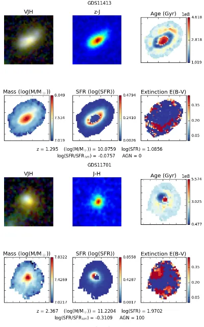
Using the median values for age, SFR, and stellar mass, resolved maps per resolution element were made from the SED fitting. The x and y pixel coordinates were plotted in a scatter plot with the corresponding physical parameter as a colorbar. The caption beneath the grid includes the redshift (z), the total stellar mass (log(M/M)), SFR (log M yr−1 ),
log(SFR/SFRM S), and AGN detection, where 100 is an X-ray detected AGN, 010 is an IR
detected AGN, and 001 is a radio detected AGN. If an AGN is detected multiple ways, it is denoted by a combination of these digits. For example, 101 corresponds to a X-ray and radio detected AGN. All pixels plotted are within the segmap of the galaxy. This creates a smooth map, per pixel, of the physical characteristics of different regions of the galaxy. Tidal tails, nuclear bulges, and star forming clumps are easily seen and can easily be compared to one another in the different maps. The full set can be found in Appendix A.
4.
Map Classification Scheme
in Figure 15. These classifications were then compared to the global galaxy properties and redshift,. Out of the 362 galaxies, 12 were contaminated due to nearby bright stars (see Figure 16) and 36 were poor fits, likely due to a bright AGN (see Figure 17). These were not included in the final classifications, leaving 314 galaxies to be classified in the following sections. 75 had failed fits in just the central regions, most likely due to a central point source. This made it difficult to classify the core color. Those were left out of the core color classifications, however they were included in the other categories, if the fit was deemed reasonable. Full maps of the 314 galaxies can be found in Appendix A.
Figure 15: A cartoon illustration of each classification category. Each galaxy was sorted into one of the subcategories in each classification category.
4.1.
Core Color
up a lot of noise. Blue cored galaxies were classified with a younger central age and a blue central region. An example is shown in Figure 19. Galaxies that have intermediate cores have slightly less mass build up in the central region, with yellow or green appearing where the core should be in the color map. This is shown in Figure 20. Galaxies with unclear core are either galaxies with no clear core appearing in the mass or age maps, are asymmetric, and have no obvious nucleus. An example is shown in Figure 21.
Figure 16: An example of a galaxy with contaminated photometry due to a nearby bright star. The grid plots the the following: Top left: VJH HST stacked images. Top middle: Color map of z-J for 1<z<2 galaxies and J-H for 2<z<3 galaxies. Top right: Stellar age map with colorbar indicating the minimum, median, and maximum ages of the galaxy. Bottom left: Stellar mass map with colorbar indicating the minimum, median, and maximum stellar masses of the galaxy. Bottom middle: SFR map with colorbar indicating the minimum, median, and maximum SFRs of the galaxy. Bottom right: Extinction map with colorbar indicating E(B-V) values of 0.05, 0.20, and 0.35 The caption below figure includes the redshift (z), total stellar mass (log(M/M)), integrated SFR (log(Myr−1), the distance from the SFMS (log(SFR/SFRM S))
Figure 17: Each map is as described in Figure 17. An example of a poor fit due to a bright AGN. The QSO can be see as a point source in the VJH image.
Figure 19: Each map is as described in Figure 17. An example of a galaxy with a blue core. In the mass and age maps, the central region is offset a bit towards the bottom of the image. The color map shows blue in that same area.
Figure 21: Each map is as described in Figure 17. A galaxy with an unclear core. In the stellar mass map, there appears to be mass build up almost the whole length of the galaxy. The color map looks to correlate with the area of star formation. This could be a galaxy with stellar mass build up at all radii, or could be very dusty, as the extinction map suggests.
4.2.
Number of Clumps
The number of clumps in each galaxy was determined, excluding the nucleus. Clumps had to clearly appear in two of the following: the color map, VJH stacked image, the mass map, or SFR map. These could be star forming clumps or a companion galaxy that appeared in the segmap. A clumpy galaxy example is seen in Figure 22. A galaxy with no clumps is seen in Figure 23.
4.3.
Location of Mass Concentration
centered in the galaxy. An example of a galaxy with a central nucleus is shown in Figure 23. This galaxy has a centered nucleus in both the mass and the age maps.
4.4.
Extent of Star Formation
Two types of star formation were considered: extended star formation and concentrated star formation. Extended star formation included star formation in a ring or disk around the galaxy. An example of a galaxy with extended star formation is shown in Figure 24. Concentrated star formation was classified based on whether or not the star formation was concentrated in one area or side of the galaxy, or had multiple clumps of star formation. Figure 22 shows an example of a galaxy classified with concentrated star formation.
Figure 23: Each map is as described in Figure 17. An example of a galaxy with no clumps. The color map, the mass map, and the SFR map are all relatively smooth and exhibit no signs of clumpiness.
5.
Results & Discussion
5.1.
Core Color
First, the galaxy core colors were analyzed. Figure 25 shows a plot of SFR versus stellar mass in three redshift bins color coded by the galaxy’s core color. Galaxies that did not have a clear core could have either double nuclei, have clumpy off-centered masses, or appear as if the mass was evenly distributed.
Figure 25: SFR/M?relation in three redshift bins, color coded by core color. White points indicate galaxies
with failed SED fits in the center region, likely due to a bright AGN. Most red cores occupy the lowest redshift, with a slight increasing fraction of unclear cores into the highest redshift bin. Black solid line is the Whitaker et al. (2014) SFMS line. Gray dashed lines are a factor of 2 above and below the SFMS.
In the lowest redshift bin, 47% of galaxies have red cores. As these galaxies are the most evolved, it is not surprising that a central nuclear region has been established. Interestingly in this sample, the galaxies farthest below and above the SFMS all had poor central fits, indicated by the white points. This seems to occur in all redshift bins. In the two higher redshift bins, there are more and more “unclear” galaxy, with 24% of galaxies having unclear cores between 1.5 < z< 2, and 28% having unclear cores between 2 <z < 3.
nearly 90% of galaxies with red cores. Also, in the largest mass bin, there were no unclear or blue cored galaxies.
Figure 27 shows the relation between a galaxy’s core color and its distance from the main sequence. Most galaxies in the sample are on the main sequence, as the majority is between the gray dashed lines. This is not surprising, as all the galaxies in the sample are star-forming and starbursts are rare (Rodighiero et al. 2011). Comparing core color and distance from the main sequence shows no real trend, except it is worth noting the galaxies with intermediate cores are the most numerous below the SFMS. These could possibly be transitioning galaxies heading into a quiescent phase.
Figure 27: A histogram illustrating the relationship between core color and distance from the main sequence. The gray dashed lines are a factor of 2 above and below the SFMS. The black line is the SFMS from Whitaker et al. (2014). There appears to be slightly more red and intermediate cores in galaxies below the main sequence.
5.2.
Clumpiness
Next, galaxies were analyzed by their level of clumpiness. A plot of SFR versus stellar mass and color coded by clumpiness is shown in Figure 28. There appears to be a very weak trend with clumpiness versus redshift, which is interesting considering many previous studies have had strong conclusions suggesting higher redshift objects contain more clumps and irregular morphologies than low redshift galaxies (e.g., Huertas-Company et al. 2016). Our findings do not agree with these other studies. The galaxies with no clumps represent 45%, 46%, and 31% in each redshift bin, respectively. This seems to show that galaxies are slightly more clumpy at the highest redshifts, 2 <z <3.
Figure 28: SFR/M? relation, color coded by the level of clumpiness. Galaxies plotted in white had poor
SED fits and were left out in the statistics. The lines here are the same as Figure 25. No trend is seen.
cores and are the least clumpy, these galaxies are most likely to begin their quenching phase first and become quiescent disks or ellipticals before the lower mass galaxies. These findings agree with the theory that higher mass galaxies are the first to quench their star formation (Saracco et al. 2012, Pan et al. 2015, Tacchella et al. 2018)
Figure 29: Level of clumpiness of a galaxy, binned by the total mass of galaxy. The high mass galaxies are dominated by red cores, with over 70% having red cores. The two lower mass bins are much more even in terms the level of clumpiness.
5.3.
Extent of Star Formation
Galaxies were classified by the extent of star formation: extended star formation or concentrated star formation. Figure 31 shows a plot of SFR versus mass for three redshift bins color coded by star formation extent.
Figure 31: SFMS color coded by extended or concentrated star formation. White points indicate galaxies that had poor SED fits and were not included in the statistics.The lowest redshift bin yields almost a 50-50 split with extended and concentrated star formation. The two higher redshifts have significantly more concentrated star formation. The lines here are the same as Figure 25.
Overall, the majority of galaxies have concentrated star formation (57%). In the lowest redshift bin, 49% of galaxies have concentrated star formation and 51% have extended star formation, as seen in Figure 32. The two higher redshift bins have significantly more galaxies with concentrated star formation. Between 2 <z <3, nearly 70% of galaxies have concentrated star formation.
On the other hand, if star formation type is plotted into bins of M?, the opposite trend
is seen. Figure 33 shows concentrated star formation decreasing while mass increases. 69% of galaxies in the highest mass bin have extended star formation, while 72% of galaxies in the lowest mass bin have concentrated star formation. This is interesting, as the fraction of galaxies is almost exactly reversed in each mass bin.
sequence. The fraction of galaxies above the +2 line with extended star formation is 9% and galaxies below the -2 line with extended star formation is 32%. The fraction of galaxies above the main sequence with concentrated star formation is 10% and the fraction below the main sequence is 19%. We expected the majority of galaxies with concentrated star formation to be above the main sequence, however the fraction is nearly identical in both bins. ULIRGs at z = 1-2 typically have more concentrated star formation due to gas and dust contracting into small regions of extreme star formation (Sanders & Mirabel 1996).
Figure 33: Star formation types, binned by total stellar mass. The galaxies that have higher stellar masses have more extended star formation.
Figure 35: SFR/M?relation, color coded by the nucleus location. Over 90% of galaxies in the lowest redshift
bin have centrally located mass concentrations. The lines here are the same as Figure 25.
5.4.
Nucleus Location
Galaxies were classified based on whether the nucleus was centrally located or off-centered in the galaxy. A plot of the SFR versus mass per redshift bin color coded by the mass location is plotted in Figure 35. Nearly all galaxies (92%) in the lowest redshift bin (1 < z < 1.5) have their mass centrally located. As the redshift increases, the fraction of galaxies with off-centered nuclei increases from 8% in the lowest redshift bin to 47% in the highest redshift bin.
Figure 36 shows central or off-central masses in bins by redshift. In the lowest redshift bin, 92% of galaxies have a centrally located mass distribution. In the highest redshift bin, this fraction lowers to 53%. Central mass still dominates the highest redshift bin, however the difference is much less drastic. It is interesting to note that the highest redshift galaxies have the most off-centered masses and the most concentrated star formation, indicative of an irregular morphology.
Centrally located masses clearly dominate in all mass bins.
Figure 38 shows the location of mass plotted in bins by distance from the main sequence. The fraction of galaxies above the +2 line with centrally located masses is 6% and the fraction of galaxies with off-centered masses is 24%. Below the -2 factor line, the fraction of galaxies with central mass locations is 27% and galaxies with off-centered masses is 15%. Off-centered masses are typically a indicator of an interaction or merger, so this may be the case with these galaxies.
Figure 37: Galaxies with centered or off-centered masses, plotted in bins of total stellar mass. A small trend is seen as the stellar mass increases, the nuclei become more central in the galaxy.
5.5.
Discussion
In regards to core color, in the two highest redshift bins (1.5 < z < 2.0 and 2.0 < z <
3.0) more “unclear” cores are seen compared to 1 < z < 1.5, with the fraction of galaxies being 24% and 28%, respectively. This seems to broadly correlate with studies finding many higher redshift galaxies having irregular morphologies (e.g., Cameron et al. 2011, Targett et al. 2012). We find that our highest redshift galaxies also have slightly greater level of clumpiness and the most off-centered mass distributions. In Cameron et al. (2011), the authors found that their sample at lower redshift (1.5 < z < 2.15) exhibited more regular morphologies at higher masses, and higher redshift galaxies (2.25 < z < 3.5) had more ir-regular and diffuse morphologies. This is interesting because our sample does show nuclei becoming more unclear with increasing redshift, however there is less of a trend with clumpi-ness and redshift. The fraction of galaxies with no clumps slightly decreases from about 45% between 1 < 2 to 31% between 2 < 3. Wang et al. (2017) investigated 77 star forming disks with an outside-in mass assembly mode, which were defined to be galaxies that have higher Hα equivalent widths in the central region of the galaxy than the surrounding disk. These authors found that galaxies with bluer cores either had a bar-like structure in the central region or had a companion galaxy that was most likely boosting star formation in that region. This could be a reason for our unclear or blue cores. Investigating the global morphology could tell us if our sample of galaxies with blue or unclear cores had a possible companion that is boosting star formation.
results, as our high mass galaxies seem to have more disk-like star formation and stellar mass build up in the core. One result from Huertas-Company et al. (2016), suggests that by z ∼ 0.5, irregular galaxies are only present with a stellar mass of 109 M
and below. Galaxies
with concentrated star formation at high redshift must transform into galaxies with normal, star forming disks and eventually could form passive disks.
While clumpiness and concentrated star formation do not seem to be correlated, concen-trated star formation and off-centered mass does seem to be related. Another result from Cameron et al. (2011) states that in galaxies at z > 1.5, there is an irregular build up of stellar mass. This is also seen in our results, as galaxies in our sample from 1.5<z<3 have significantly more off-centered nuclei than galaxies from 1 < z <1.5. We also find that the higher redshift galaxies show more concentrated star formation. These could be star forming clumps in a disk that we cannot see due to poorer resolution for higher redshift galaxies. Wutys et al. (2013) theorizes that most stars were formed in a disk component during the epoch of star formation. Some of these clumps could also be obscured by dust, which is not well-constrained in our study.
Mergers could be the reason that the galaxies above the SFMS had more concentrated star formation and off-centered mass distributions. There are 42 galaxies in our sample that lie above the factor of two line. Figure 39 shows a subsample of those 42 galaxies. Many of these galaxies have clear companions or look very irregular in shape. Many galaxies also exhibit tell-tale signs of mergers such as tidal tails.
having more extended star formation (Rujopakarn, Rieke, Eisenstein, & Juneau 2011). It is not surprising that only a small fraction of our sample is above the SFMS by a factor of 2, and therefore considered starbursts. Starbursts are rare and only occur for a very short time during the merger process. Many of our galaxies below the SFMS could be transitioning from a starbursting phase into the quiescent phase.
Figure 39: A subset of 18 galaxies taken from the 42 starburst galaxies. Many are seen with companions, indicating interactions while others are seen with tidal tails and irregular morphologies which are indicative of mergers.
6.
Future Work
In order to ensure the quality of the SED fits, we would like to perform further error analysis of our work. We would perform a signal-to-noise cut on our sample and only fit pixels above the 3σ limit. From these SED fits we will use the outputs to create noise maps for each of the measured quantities.
Morphology and interaction class can also be compared to all of these resolved maps. This could give us the number of possible mergers that are in our sample. Comparing global and local morphology could unveil trends that are worth investigating further.
7.
Summary
In a sample of 362 Herschel-selected galaxies in CANDELS/GOODS-S, we perform re-solved, pixel-by-pixel SED fits to study the relation between global and local properties of galaxies. VJH stacked HST images, rest frame U-V color maps, and resolved maps of stellar age, stellar mass, SFR, and E(B-V) were made to study galaxy’s substructure on kiloparsec scales. From these maps, galaxies were classified by eye in four categories: core color, level of clumpiness, type of star formation, and location of mass concentration. We find that most high redshift galaxies (1.5 < z < 3) have the most concentrated star formation and many have off-centered masses, suggesting there are more irregular morphologies present at high redshift. We find that most high mass galaxies have central nuclei, extended star formation, no clumps, and red cores indicating these high mass galaxies have and will build up all their stellar mass before the lower mass galaxies. Many of these high mass galaxies could also have undergone mergers in a previous epoch and irregular star forming clumps have since spread into a disk of star formation.
References
Astropy Collaboration, 2013, A&A, 558, 33
Astropy Collaboration, 2018, AJ, 156, 3
Balestra, I., et al. 2010,A&A, 512, 12
Balogh, M., et al. 1999,ApJ, 527, 1
Balsara, D., Livio, M., & O’Dea, C.P., 1994, ApJ,
437, 1
Baugh, C.M., Cole, S., & Frenk, C.S., 1996,
MN-RAS, 283, 1361
Bedregal, A.G., et al. 2013,ApJ, 778, 126
Bell, E., et al. 2004b,ApJ, 608, 2
Bell, E., et al. 2005,ApJ, 625, 23-36
Blanton M.R., et al. 2003,ApJ, 592, 819-838
Blanton, M.R., 2006, ApJ, 648, 268-280
Brammer, G, et al. 2009,ApJ, 706, 1
Brennan, R., et al. 2015,MNRAS, 251, 2933-2956
Bruzual G., & Charlot, S., 2003, MNRAS, 344, 4
Cano-D´ıaz M., et al. 2016,ApJ, 821, L26
Cameron, E., et al. 2011,ApJ, 743, 146
Capellutti, N., et al. 2016,ApJ, 823, 95
Chabrier, G., 2003,PASP, 115, 763
Cooper, et al. 2012,MNRAS, 425, 2116
da Cunha E., Charlot, S., & Elbaz, D., 2008,
MN-RAS, 388, 1595
Daddi, E., et al. 2007,ApJ, 670, 156
Darvish, B., et al. 2016,ApJ, 825, 2
Dasyra, K.M., et al. 2008,ApJ, 680, 232
Davis, M., et al. 2007, et al.ApJL, 660, L1
Dekel, A., & Birnboim, Y., 2006,MNRAS, 368, 1
Dekel, A., et al. 2009a,Nature, 457, 451-454
Dekel, A., Sari, R., & Ceverino, D.,ApJ, 703, 1
De Lucia, G., Springel, V., White, S.D.M., Croton,
D., Kauffman, G., 2006,ApJ, 366, 499-509
Doherty, et al. 2005,MNRAS, 361, 525
Donley, J.L., et al. 2012,ApJ, 748, 142
Elbaz, D., et al. 2011,A&A, 533, A119
Elmegreen, B.G., Bournaud, F., & Elmegreen D.M.,
2008,ApJ, 688, 1
Elmegreen, D.M., Elmegreen, B., Ravindranath, S.,
& Coe, D., 2007,ApJ, 658, 2
Faber, S., et al. 2007,ApJ, 665, 1
Finkelstein, S., et al. 2012,ApJ, 756, 2
Gabor, J.M., Dave, R., Finlator, K., &
Oppen-heimer, B.D., 2010, MNRAS, 407, 2
Genel, S., et al. 2008,ApJ, 789-793
Giavalisco, M., et al. 2004, ApJ, 600, L93-L98
Grogin, N., et al. 2011, ApJS, 197, 2
Guo, Y., et al. 2013, ApJS, 1308, 4405
Hemmati, S., et al. 2014,ApJ, 797, 108
Herenz, et al. 2017,A&A, 606, A12
Hopkins, P., Herquist, L., Cox. T., & Keres, D.,
2007,ApJS, 175, 2
Hubble, E.P., 1926,ApJ, 64, 321
Huertas-Company, M., et al. 2016, MNRAS, 462,
4495
Inami, et al. 2017,A&A, 608, A2
Kartaltepe, J.S., et al. 2012,ApJ, 757, 23
Kartaltepe, J.S., et al. 2015, ApJS, 221, 11
Kartaltepe, J.S., et al. 2019, in prep.
Koekemoer, A., et al. 2011, ApJS, 197, 2
Kriek, M., et al. 2008,ApJ, 677, 1
Kriek, M., et al. 2015,ApJS, 218, 15
Kurk, et al. 2013,A&A, 549, 63
Laughlin, G., Bodenheimer, P., & Adams, F., 1997,
ApJ, 482, 1
Lawrence, A., et al. 2007,MNRAS, 379, 1599
LeFevre, O., et al. 2004,A&A428, 1043
LeFevre, O., et al. 2015,A&A576, A79
Le Floc’h, E., et al. 2005,ApJ, 632, 1
Lofthouse, E.K., Kaviraj, S., Conselice, C.S.,
Mort-lock, A., & Hartley, W., 2017, MNRAS, 465,
2895-2900
Madau P., & Dickinson, M., 2014,A&A, 52, 415-486
Margalef-Bentaol, B., et al. 2016,MNRAS, 461, 3
Magnelli, B., et al. 2011,A&A, 528, 35
Magnelli, B., et al. 2013,A&A, 553, A132
McLure, et al. 2018,MNRAS, 479, 25
Miller, N.A., et al. 2013,ApJS, 205, 13
Momcheva, et al. 2016,ApJS, 225, 27
Morris, A.M., et al. 2015,AJ, 149, 178
Mosleh, M., et al. 2017,ApJ, 837, 2
Noeske, K., et al. 2007,ApJ, 660, 43
Oesch, P.A., et al. 2010,ApJL, 714, 1
Pan et al. 2015,ApJ, 804. 42
Papovich, C., Dickinson, M., Giavalisco, M.,
Con-selice, C.J., & Ferguson, H.J., 2005, ApJ, 631,
101-120
Pentericci, et al. 2018,A&A, 616, 174
P´erez, E., et al. 2013,ApJL, 764, L1
Pilbratt, G.L., et al. 2010,A&A, 518, L1
Robitaille T.P. & Whitney, B.A., 2010, ApJL, 710,
1
Rodighiero, G., et al. 2011,ApJ, 739, 2
Rujopakarn, W., Rieke, G.H.,, Eisenstein, D.J., &
Juneau, S., 2011,ApJ, 726, 93
S´anchez-Bl´azquez, P., Forbes, D., Strader, J., &
Brodie, J., 2007,MNRAS, 377, 2
Sanders, D.B. & Mirabel, I.F., 1996,ARAA, 34,
749-792
Santini, P., et al. 2009,A&A, 504, 751-767
Saracco, P., Gargiulo A., & Longhetti, M., 2012,
MNRAS 422, 4
Scoville, N., et al. 2007,ApJS, 172, 1
Shapiro, K., et al. 2008,ApJ, 682, 1
Silverman, J.D., et al. 2010,ApJS, 191, 124
Sparre, M., et al. 2015,MNRAS, 447, 3548-3563
Strateva et al. 2001,AJ, 122, 1861-1874
Szokoly, G.P., et al. 2004,ApJS, 155, 271
Tacchella S., et al. 2015,Science, 348, 6232
Tacchella, S., et al. 2016,MNRAS, 458, 1
Tacchella, S., et al. 2018,ApJ, 859, 1
Targett, T.A., et al. 2012,MNRAS, 432, 3
Trump, J., et al. 2013,ApJ, 763, 6
Vanzella, et al. 2008,A&A478, 83
Whitaker, K., van Dokkum, P., Brammer, G., &
Franx, M., 2012,ApJL, 754, 29
Whitaker, K., et al. 2014,ApJ, 795, 2
Wild, V., et al. 2016,MNRAS, 463, 832-844
Wolf, C., et al. 2004,A&A, 421, 913
Wutys, S., et al. 2008,ApJ, 682, 985
Wutys, S., et al. 2011,ApJ, 742, 96
Wutys, S., et al. 2013,ApJ, 779, 135
Zaragoza-Cardiel, J., et al. 2018,ApJS, 234, 35
Zheng, X.Z., et al. 2004,A&A, 421, 847-862
Appendix A
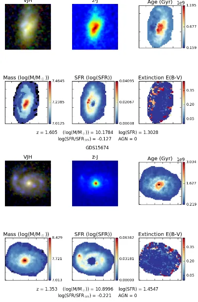
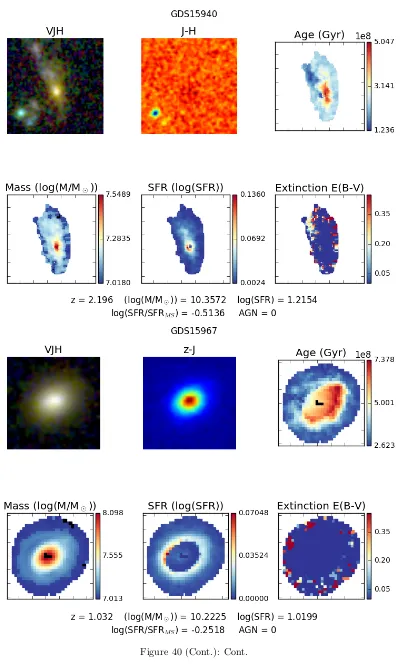
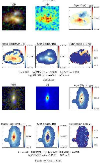
Figure 40: Top left: VJH HST stacked images. Top middle: Color map of z-J for 1 <z<2 galaxies and J-H for 2<z<3 galaxies. Top right: Stellar age map with colorbar indicating the minimum, median, and maximum ages of the galaxy. Bottom left: Stellar mass map with colorbar indicating the minimum, median, and maximum stellar masses of the galaxy. Bottom middle: SFR map with colorbar indicating the minimum, median, and maximum SFRs of the galaxy. Bottom right: Extinction map with colorbar indicating E(B-V) values of 0.05, 0.20, and 0.35 The caption below figure includes the redshift (z), stellar mass (log(M/M)),
SFR (log(M yr−1), the distance from the SFMS (log(SFR/SFRM S)) where negative numbers are below