Essays on Bond Yields

Essays on Bond Yields

Vijay Austin Murik

November 2011

Declaration

The work in this thesis is my own except where otherwise stated.

Acknowledgements

I would like to express profound gratitude to my Supervisor at the Australian National University, Professor Tom Smith, for unwavering encouragement and inspiration through the course of my Ph.D. research. It has been an absolute pleasure to undertake my Ph.D. under Tom’s expert guidance. Tom introduced me to the highest ideals of research, and taught me how to think about financial markets and the economy. I feel very fortunate to be Tom’s student. I am also grateful to the other members of my supervisory panel, Professor Doug Foster and Professor Garry Twite, for their assistance and encouragement during my studies.

I would like to thank my present and past managers at the Australian Office of Financial Management: Michael Bath, Megan Hardy, Matthew Wheadon, H¨ulya Yilmaz and David Ziegler for their support of my academic endeavours and career aspirations over the past five years, and for sharing their perspectives on how fixed-income and securitisation markets function in practice.

I would like to acknowledge financial support in the form of a Ph.D. schol-arship from the ANU College of Business and Economics, and also flexible study leave arrangements from the AOFM.

I would like to thank Jonathon McGrath for many thought-provoking discussions about the nature of financial markets over the past few years, and Nicole Neveu for her wisdom and encouragement.

Contents

Abstract viii

1 Introduction 1

2 Bond pricing with a surface of zero coupon yields 8

2.1 Introduction . . . 8

2.2 Zero coupon yield surface . . . 11

2.3 Risk premia in Australian bond yields . . . 14

2.4 Conclusion . . . 23

3 Conditional tests of monotonicity in term premia 28 3.1 Introduction . . . 28

3.2 Determinants of term premia . . . 31

3.3 Monotonicity tests . . . 33

3.4 Monotonicity in U.S. term premia . . . 36

3.5 Conclusion . . . 43

4 Measuring monetary policy expectations 50 4.1 Introduction . . . 50

4.2 Measuring expectations . . . 53

4.3 The fixed income universe . . . 57

4.4 Expectations in Australian bond pricing . . . 58

4.5 Conclusion . . . 72

5 Conclusion 74

List of Tables

2.1 Descriptive statistics, surface fitting errors (per cent) . . . 17

3.1 Descriptive statistics, sample term premia (per cent) . . . 38

3.2 Correlation matrix: excess returns and factors . . . 39

3.3 Monotonicity test p-values, by conditioning factor . . . 40

3.4 Empirical power: Frequencies of monotonicity outcome in tests . . . 42

4.1 Forecast error descriptive statistics . . . 62

4.2 OLS estimates for equation (4.1) . . . 64

4.3 GMMIV estimates for moment conditions (4.3) . . . 68

List of Figures

2.1 Observed yield curves, 31 March 2011 . . . 15

2.2 Zero coupon surface, 31 March 2011 . . . 16

2.3 Decomposition, Treasury Corporation of Victoria yields . . . 18

2.4 Decomposition, Inter-American Development Bank yields . . . 19

2.5 Decomposition, European Investment Bank yields . . . 20

2.6 Relative pricing, long semi-government bonds . . . 22

2.7 Relative pricing, short supranational and agency bonds . . . 23

3.1 Sample mean term premia . . . 37

3.2 Sample mean conditional term premia . . . 39

4.1 Fixed income market pricing . . . 59

Abstract

This doctoral dissertation comprises three essays which study the determinants of bond yields.

The dissertation is organised around the idea that bond yields can be partitioned into a risky component which prices for the risk of illiquidity and default; and a risk-free component which prices for investors’ time preferences, and expected monetary policy movements (Homer and Leibowitz, 2004). The first essay considers the liquidity and credit premia in supranational, semi-government and agency bond yields; term premia in sovereign bond yields and their relation to the economy constitute the focus of the second essay; and the third essay is devoted to an inquiry into the nature of expectations of future monetary policy movements in bond yields.

The second essay designs conditional tests for the liquidity preference hypothesis, which predicts monotonicity in term premia. Drawing on the excess return forecasting literature (Cochrane and Piazzesi, 2005; Ludvigson and Ng, 2009), the tests are conditioned on information from macroeconomic variables and the current yield curve. Specifically, a filter is constructed to use this conditioning information set in new versions of the Wolak test (Boudoukh et al., 1999a) and Monotonicity Relation test (Patton and Timmermann, 2010) for the liquidity preference hypothesis. Consistent with the literature, our tests conclude that raw, unconditional term premia in U.S. Treasury bills between 1965 and 2001 do not increase monotonically. However, we find that the tests indicate term premia in Treasury bills do increase monotonically when the sample term premia are conditioned on the excess return forecasting factors. This confirms the explanatory power of the excess return forecasting factors, and also suggests that conditioning information should be used in applying inequality constraints tests to determine whether the liquidity preference hypothesis holds empirically.

Chapter 1

Introduction

The bond market lies at the intersection between the real economy and finan-cial markets. With regard to the economy, the risk-free Treasury yield curve responds to shocks in inflation and growth expectations. The benchmark provided by the yield curve underpins all other interest rates in the economy, and thus determines the supply and price of credit. There is a strong relation-ship between the business cycle and the yield curve. The supply of bonds is determined by fiscal policy, and monetary policy influences the short end of the yield curve. Offshore flows of funds to and from the domestic bond market constitute an important determinant of the capital account in the balance of payments.

Turning to financial markets, the risk-free yield curve sets the discount factors according to which all other financial assets are priced. The yield curve thus determines the time value of money. In a very broad sense the cashflows of almost any financial security (and by extension, any government, corporate or trust structure) can be treated as a bond or bond option. Furthermore, derivatives and securitisation technologies provide almost unlimited flexibility to market participants in structuring fixed income securities to meet their investment, financing and hedging requirements. It is therefore clear that the bond market plays a fundamental role in the valuation of all financial securities in other financial markets.

ascribe a value to the deterministic or risky sets of cashflows that are attached to fixed income securities. This dissertation explores empirical aspects of bond market pricing. The underlying philosophy of our research is that raw market pricing is informative: important information about investors’ risk sentiment and interest rate, inflation and growth expectations can therefore be extracted from observed market pricing with minimal interference from models.

Specifically, in this dissertation, we consider how the bond market prices for risk. The aim is to measure and characterise the credit and liquidity premia in Australian dollar denominated semi-government, supranational and agency bonds (Chapter 2); the term premia in U.S. Treasury bills (Chapter 3); and the expectations of future monetary policy movements in various Australian fixed income instruments and interest rate futures (Chapter 4). In each case, we find that valuable information can indeed be extracted from the market pricing implied by bond yields. The remainder of the present Chapter provides an overview of the research problem, methodology, findings and significance of each Chapter in the dissertation.

Chapter 2, ‘Bond pricing with a surface of zero coupon yields’, explores whether the fixed income market prices in a consistent manner Treasury bonds along with other bonds of different credit qualities and with different liquidity characteristics. A model is proposed for risk free zero coupon yields, credit premia and liquidity premia for all tenors across all securities in the entire fixed income market at a single point in time.

of multivariate smoothing splines to yield curve estimation (Krivobokova et al., 2006).

To implement the model, we use end-of-day market yields for bonds issued by a wide range of issuers as the key input for the model. Zero coupon yield curves are then estimated for each issuer’s bonds with a standard bootstrap and smoothing splines interpolation (starting with the risk-free Treasury zero curve) (Hagan and West, 2006). Next, we compute risk free asset swap margins for each bond. These are margins to the floating rate on an interest rate swap based on the Treasury zero curve that match exactly the cash flows of the bond (Manning, 2004). We fit an approximation to a multivariate smoothing spline (a thin plate regression spline) through the cloud of points to get a zero coupon surface (Wood, 2003). Given the surface and the underlying zero coupon bond yields, we can then assess how well the surface prices bonds and swaps. For each issuer, we also solve for the constant risk free asset swap margin that best prices its bonds off the zero coupon surface. This margin is the fundamental measure of the credit premia, and the zero coupon yield errors to the surface are the fundamental measures of liquidity premia.

We find that the zero coupon yield surface summarises effectively the information in traded yields from the semi-government, supranational and agency segment of the Australian fixed income market. Looking at the quarter-end fit of the surface from 2008Q1 to 2011Q1, it is clear that the disruption in pricing through the Global Financial Crisis affects the surface; but that the surface still captures much of the cross-sectional variation in bond yields for different issuers. Furthermore, the surface can be used to provide decompositions of traded bond yields into a risk-free component plus premia for credit and liquidity. We explore the decomposition in a cross-sectional (yield curve) sense and in a time series sense for selected bond lines of a prominent issuer. The decomposition shows how credit yield premia widened during the Crisis, but there were liquidity yield discounts for high quality semi-government, supranational and agency bonds.

dimensional surface that can be decomposed into term premia (the pure time value of money component), credit premia (associated with default risk) and idiosyncratic liquidity premia.

Chapter 3, ‘Conditional tests of monotonicity in term premia’, considers the expected shape of term premia in U.S. Treasury bills across tenors, drawing on the econometric methodology of multiple inequality constraints testing. Existing specifications of inequality constraints tests for monotonicity in term premia (Boudoukh et al., 1999a; Patton and Timmermann, 2010) suffer from low power because they utilise an insufficient set of conditioning information. Hence, we improve the tests by incorporating excess return forecasting factors from the forward curve (Cochrane and Piazzesi, 2005); and factors estimated via principal components analysis from a large panel of macro variables as conditioning information (Ludvigson and Ng, 2009).

An inequality constraints test for term premia conditioned on macro and forward curve factors is the logical next step in relation to at least three strands of the literature. First, the literature on excess return forecasting factors does not consider the conditional shape of premia across tenors (Ludvigson and Ng, 2009; Cochrane and Piazzesi, 2005; Duffee, 2011). Second, scholarship on inequality constraints testing does not accommodate the use of principal components as conditioning information (Boudoukh et al., 1999a; Patton and Timmermann, 2010). Third, the literature on arbitrage free term structure modelling does not address traditional theories about the term structure, instead adopting parametric forms for risk premia that do not necessarily reflect empirical term structure dynamics (eg. Joslin et al., 2010, 2011).

of the conditional tests with those of the unconditional tests, and perform a simulation study to assess the empirical power of the two tests, with and without the use of the conditioning information.

Our tests suggest that the use of conditioning information changes the outcome of the tests from the unconditional case. Both the Monotonicity Relations Test and the Wolak Test suggest that U.S. Treasury bill term premia are non-monotonic using the unconditional sample. However, when we condition our tests on the positive elements of the Cochrane and Piazzesi (2005) and Ludvigson and Ng (2009) factors in particular, the tests suggest that the conditional term premia are monotonically increasing. This is evidence that the excess return forecasting factors do have explanatory power in respect of the conditional shape of term premia. Further, our results imply that the conditional tests shed new light on how the monotonicity tests can be applied to term premium data, by better capturing the information that market participants are ostensibly considering when they determine U.S. Treasury bill pricing. The simulation experiments then show that the conditional tests are more powerful in detecting monotonicity than their unconditional equivalents.

More generally, our approach to testing for the conditional shape of term premia across tenors provides an effective method for empirically characterising term premia, and thereby describing the evolution of the yield curve over time in terms of departures from the expectations hypothesis. Our approach does not impose the ´a-priori structure of an arbitrage free term structure model, and yet it allows for statistically powerful tests of hypotheses about the ex ante shape of term premia across tenors.

Chapter 4, ‘Measuring monetary policy expectations’, assesses the accuracy of the Australian fixed income market in pricing for future movements in the monetary policy instrument. We develop an econometric framework for measuring monetary policy expectations from fixed income pricing that is well founded in asset pricing theory. The framework allows us to abstract away from risk premia in market pricing, and also facilitates the measurement of hitherto elusive long term interest rate expectations of horizons between one and three years.

expectations from fixed income securities without using the prism of a term structure model. The literature on extracting policy expectations from asset prices is mainly limited to money markets and related futures contracts (eg. Kuttner, 2001; Taylor, 2010). While money markets and short term interest rate futures have a direct relation to the policy instrument, they often suffer from a lack of liquidity and are therefore subject to additional risk premia (Piazzesi and Swanson, 2008).

Our econometric framework provides a mechanism for comparing yields and implied forward rates associated with market pricing for various types of Australian fixed income securities with the ex-post average cash rate over the same period. The universe of fixed income securities under consideration in our study includes: overnight indexed swaps, interbank futures, bank bills, bank bill futures, and Treasury bond futures. Once we have calculated the yields from market prices on the one hand, and corresponding average cash rates on the other, we compute cash rate forecast errors for each type of fixed income security at each observation date. This leads to root mean squared forecast errors for each type of fixed income security. Also, in a simple attempt to abstract away from risk premia down to a linear approximation, we regress the cash rate returns onto the yields and forwards. Then, to provide further robustness around our results, and better control for the effects of risk premia, we use a generalised method of moments instrumental variables estimation framework. Under this framework, the yields and forwards of securities that are subject to term, credit and liquidity risks are instrumented with other yields and forwards that are not subject to those risks. In this manner, we improve on the simple regression framework that has been adopted by most other studies of market-based measures of monetary policy expectations (G¨urkaynak et al., 2007; Goodhart and Lim, 2011).

these regressions still leave much of the variation in the cash rate unexplained. This is because, beyond the horizon of six months, the presence of risk premia diminishes to a large extent the signal on expectations in market pricing. Nonetheless, our instrumental variables framework suggests there is valuable information embedded in pricing on three and ten year bond futures contracts regarding expected cash rate movements over the one to three year horizon.

Chapter 2

Bond pricing with a surface of

zero coupon yields

2.1

Introduction

Each trade in the fixed income market represents an individual market par-ticipant’s view on the time value of money, and the amount of compensation required by investors for taking on credit and liquidity risk. Nonetheless, bond market pricing is not determined in isolation from one trade to the next. To the extent that it is an efficient market, the fixed income market does not just price consistently between the different securities of the same issuer — it prices consistently between the securities of different issuers. At a single point in time, the market’s pricing for sovereign, semi-sovereign, bank and corporate bonds is jointly determined. The principal argument of this essay is that the fixed income market differentiates between security specific characteristics in a consistent manner, and applies the same approach to pricing for risk between different fixed income securities.

yield curves? From the econometrician’s perspective, this means that if the zero coupon yield curves of different issuers are placed side by side (in order of credit risk) in a three dimensional space with axes for tenor, credit risk and zero coupon yields, it should be possible to fit a smooth surface through the yield curves. Such a surface would then summarise all of the discount factors that are being used to price traded bonds in the market.

Our argument constitutes a fundamental challenge to the extant literature on fixed income market valuation. To date, authors have focused on single aspects of the fixed income market in isolation.1 _{There are growing bodies of}

scholarship aiming to measure and explain credit spreads (Martell, 2008; Liu et al., 2009; Jacoby et al., 2009; Krishnan et al., 2010), and liquidity premia (Chordia et al., 2005; Chen et al., 2007; Goyenko et al., 2010; Bao et al., 2011) in bond yields, that complement, but do not address directly the underlying literature on zero coupon yield curve estimation from risk free Government bond yields (Fama and Bliss, 1987; Nelson and Siegel, 1987; Fisher et al., 1994; Anderson and Sleath, 2001; Hagan and West, 2006) and defaultable bond yields (Houweling et al., 2001; Jarrow et al., 2004; Jarrow, 2004; Jankowitsch and Pichler, 2004; Cruz-Marcelo et al., 2011). However, if risk free zero coupon yields, credit premia and liquidity premia are determined jointly across the fixed income market, then the extant literature is not taking into account the fundamental interactions between these quantities that influence market valuations.

Accordingly, we present a unified method that prices simultaneously all risk free and defaultable bonds in the market, and thereby leads to consistent measures of credit and liquidity premia. Under this method, a smooth surface is fit through a three dimensional cloud of zero coupon yields. The co-ordinates of these zero coupon yields within the cloud are determined by their tenor and their risk free asset swap margin, which is the margin to the floating rate for an interest rate swap based on the risk free zero coupon yield curve that matches exactly the cash flows of the underlying bond. The smooth surface is

1_{This is no surprise, given that credit and liquidity premia cannot be directly observed}

then modelled as a thin plate regression spline, which is an approximation to a multivariate smoothing spline. Constructed in this manner, such a “zero coupon yield surface” constitutes a model of all zero coupon yield curves (equivalently, discount factors) in the market. Under additional identification assumptions, the model can then be used to decompose traded bond yields into a risk free component plus premia for credit and liquidity. The zero coupon yield surface is an important extension of extant methods in fixed income analysis, where zero coupon yield curves are typically estimated only from Government bond yields and interest rate swap yields. Our technique generalises traditional bootstrap and interpolation methods (Hagan and West, 2006) to other fixed income securities, and facilitates the decomposition of traded bond yields into their basic constituents.

We find that the zero coupon yield surface provides an accurate char-acterisation of the information in traded yields from the semi-government, supranational and agency (SSA) segment of the Australian fixed income mar-ket. The root mean squared fitting errors of the surface over 2008Q1 to 2011Q1 hit their peak of 15 basis points at the height of the Global Financial Crisis in 2009Q2, but quickly recede thereafter. We show that despite the market turbulence, the surface still captures much of the cross-sectional variation in bond yields across different issuers. Furthermore, we use the surface to decom-pose traded bond yields into a risk-free component plus premia for credit and liquidity. We explore the decomposition in both a cross-sectional (yield curve) sense and in a time series sense for selected bond lines of three prominent issuers. The decomposition shows how credit premia spiked during the Crisis, but the impact on pricing was dampened by the presence of liquidity discounts for high quality SSA bonds. This is consistent with investor sentiment through the Crisis period, where SSA bonds were perceived by portfolio managers as a safe haven asset class.

decompose traded bond yields under additional identification assumptions. Finally, Section 2.4 concludes.

2.2

Zero coupon yield surface

2.2.1

Zero coupon yields

At the outset, we bootstrap zero coupon yields from traded bond yields for each issuer across the market, using linear interpolation on log discount factors. This is a standard technique in fixed income analysis, and is well documented in eg. Hagan and West (2006) and Fama and Bliss (1987) (details are provided in the Appendix). This gives us separate zero coupon yield curves for each issuer in the market.

2.2.2

Risk free asset swap margins

Once zero coupon yields have been computed for each of the issuers in the fixed income market, the next step is to calculate the measure of credit risk. This measure is used to project the zero coupon yields into a three dimensional space with axes for yield, tenor and credit risk. The relevant measure of credit risk to be used is theriskfree asset swap margin, which is an asset swap margin using a swap based on the Treasury zero coupon yield curve.2

These asset swap margins are a purely market-based measure of credit risk, which are superior to alternatives such as credit ratings, benchmark par yield spreads, exchange for physical spreads and zero coupon yield spreads. This is because asset swap margins take account of the cash flows of the underlying securities; and they can measure credit risk for any fixed income security given its market price.

2_{An asset swap is a type of trade in the fixed income market where the investor purchases}

With their flexibility in mind, we use riskfree asset swap margins to assess the credit risk of risky bonds relative to the risk free Government zero coupon yield curve. The riskfree asset swap margin is calculated with the discount factors taken from the riskfree zero coupon yield curve, and using the market prices of defaultable bonds across the cross-section of issuers in the fixed income market.

2.2.3

Surface interpolation method

Define rit and χit as the zero coupon yield and risk free asset swap margin

associated with issuer iat tenor t. Having obtained zero coupon yields and risk free asset swap margins, we project triplets of zero coupon yields, risk free asset swap margins and tenors into three dimensional space. Then we fit the smooth surface g through these triplets. The surface takes the form of a thin plate regression spline (Wood, 2003).3

Specifically, we estimate the bivariate thin plate regression spline

rit =g(t, χit) +it (2.1)

through the triplets of zero coupon yields, tenors and asset swap margins {rit, t, χit}, and the resulting zero coupon yield surface summarises the entire

set of zero coupon yield curves for the fixed income market.

The errors it are crucial to the analysis of the zero surface. Clearly, small

errors indicate a close fit, and therefore constitute evidence of consistency in fixed income market pricing from one issuer to the next.

2.2.4

Credit and liquidity yield premia

Beyond summarising the information in individual issuers’ zero coupon yield curves, the zero coupon yield surface fulfills another important function. It allows for traded yields to be decomposed into a risk free component along

3_{The construction of the splines is covered in the Appendix, here it suffices to describe}

with premia for credit risk and liquidity risk. This depends on additional assumptions.

Now, the risk free asset swap margins as calculated for each traded bond conflates credit and liquidity premia, and is not a pure credit spread. This is because it captures the difference between the price and the risk free price, which could involve either credit or liquidity premia. Given the zero coupon yield surface, we implement the decomposition of observed bond prices with

pit =p(itγ)−p

(χi)

it −p

(λit)

it , (2.2)

where pit is the observed bond price, p

(γ)

it represents the net present value

of the bond’s cashflows using discount factors from the riskfree zero coupon yield curve; p(χi)

it is a price discount (yield premium) for credit risk, and p

(λit)

it

is a price discount (yield premium) for liquidity risk. To be explicit, this specification is predicated on the assumption that the risk-free component of bond yields is additive with the credit risk and liquidity risk price discounts, and that together all three components sum to the observed bond price.4

Now, we estimate the pure credit price discountp(χi)

it by solving the problem

p(χi)

it ≡p

(γ)

it −pit(g(t, χi)), χi : min

χ kpi−pi(g(t, χ))k, (2.3)

where pi is a vector containing the observed prices pit for all bonds associated

with issuer i. Also,pi(g(t, χi)) denotes the prices of the same bonds calculated

with the estimated zero coupon surface using the discount factors corresponding to the points on the surface with tenor equal to t and constant riskfree asset swap margins equal to χi.5 Hence the credit price discount for a bond is its

4_{Our intention here is not to assert that this is the only way or the correct way to}

decompose bond yields with the zero coupon surface, but to show that this is one possible approach to decomposition using the surface. Of course, this additive decomposition would be expected to be valid only in fixed income markets where there are few liquid bond lines per issuer, and where extrinsic considerations such as tax, operational and sovereign risk are not influential in pricing. This is reasonable for well developed fixed income markets such as Australia.

5_{Geometrically,g(t, χ}

i) can be represented as selecting the “slice” of the zero coupon

risk free equivalent price less its pure credit price, where the latter is priced off the zero coupon yield surface along a single risk free asset swap margin. This is consistent with the situation where the market prices equally for credit risk across tenors.

The liquidity price discount is then the idiosyncratic remainder between the risk free price less the observed price on the one hand and the pure credit price discount on the other, according to the decomposition (2.2), so that

p(λit)

it =p

(γ)

it −pit−p(itχi). (2.4)

These credit and liquidity premia can also be expressed in yield to maturity terms by treating p(_it·) as the price in the bond pricing formula (see equation (2.7) in the Appendix) and then solving for the yield to maturity yit given the

underlying cash flows.

We have shown that observed bond yields can be decomposed into a risk free component along with premia for credit risk and liquidity risk in the manner described in this Section. The separation between credit and liquidity premia is achieved through the use of a constant risk free asset swap margin. The difference in par yield terms between the pure credit price and the risk-free price is the credit premium; and the difference in par yield terms between the market price and the pure credit price is the liquidity premium. Taking a step back, it is clear that our decomposition method imposes minimal structure on traded bond yield data, and yet provides an effective means through which to extract credit and liquidity premia.

2.3

Risk premia in Australian bond yields

In this Section, we start by motivating the need for our method in practice. Then we fit the zero coupon yield surface to Australian fixed income market end of quarter revaluation pricing (2008Q1 to 2011Q3), as sourced from Yieldbroker, and show an example of our decomposition method with Treasury Corporation of Victoria bond yields and the zero coupon surface. We have

restricted our sample to sovereign risk free bonds, semi-government bonds, and supranational/agency bonds. The sample covers a total of 13 quarters, with 37 unique issuers from the semi-government, supranational and agency segment of the bond market, and 1,941 observations of end of quarter bond yields.

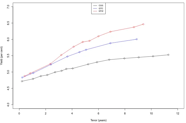
The fixed income market pricing implied by observed yield curves incor-porates a lot of information, not all of which is obvious. Figure 2.1 shows Australian Government yields, as compared to Queensland Treasury Corpora-tion (QTC) yields and Kreditanstalt fur Wiederaufbau (KfW) yields. This Figure illustrates market pricing for the bonds of each of the three issuers, and therefore contains sufficient information for one to analyse whether the market is pricing consistently for each issuer’s bonds. However, it is not obvious how consistency in pricing should be assessed just by looking at the observed yields (eg. is there an investment reason why QTC spreads are lower than KfW spreads by the amount observed?). Further, the presence of coupons distorts comparison between observed yields, and it is impossible to distinguish credit spreads from liquidity spreads in Figure 2.1.

Figure 2.1: Observed yield curves, 31 March 2011

0 2 4 6 8 10 12

4.0

4.5

5.0

5.5

6.0

6.5

7.0

Tenor (years)

Y

ield (per cent)

CGS QTC KFW

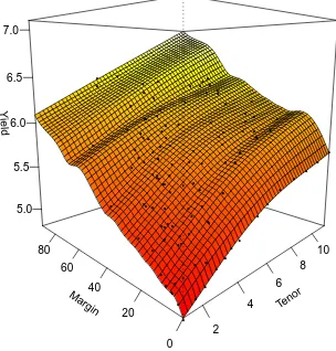
surface makes it possible to assess consistency in the fixed income market and decompose bond yields. Fundamentally, the surface is the true primitive of the fixed income market, showing discount factors for all credit qualities at all tenors. An example of the zero coupon surface is set out in Figure 2.2. Intuitively, this graph shows that as far as the eyeball test is concerned, the

Figure 2.2: Zero coupon surface, 31 March 2011

Tenor 2 4 6 8 10 Margin 0 20 40 60 80 Y ield 5.0 5.5 6.0 6.5 7.0 ● ● ● ● ● ● ● ● ● ● ● ● ● ● ● ● ● ● ● ● ● ● ● ● ● ● ● ● ● ● ● ● ● ● ● ● ● ● ● ● ● ● ● ● ● ● ● ● ● ● ● ● ● ● ● ● ● ● ● ● ● ● ● ● ● ● ● ● ● ● ● ● ● ● ● ● ● ● ● ● ● ● ● ● ● ● ● ● ● ● ● ● ● ● ● ● ● ● ● ● ● ● ● ● ● ● ● ● ● ● ● ● ● ● ● ● ● ● ● ● ● ●

surface fits zero coupon yields fairly closely in March 2011. The remainder of this Section is devoted to showing how surfaces like the one above fit Australian fixed income market pricing data through time, and how they can be used to decompose bond yields.

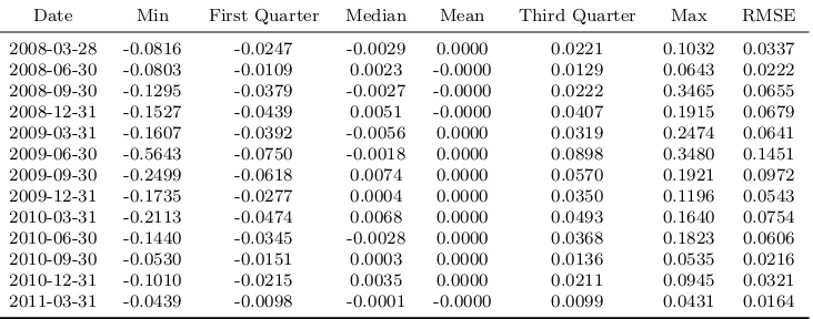
statistics for errors it are provided in percentage terms by the Table 2.1. As

can be seen, the mean errors are all close to zero, indicating the surface is unbiased. The quartiles show that the errors are relatively symmetric around zero, but the minima and maxima do indicate the presence of a few outliers on each sample date. Further, the root mean squared errors are all small, but they did increase to a peak of 15 basis points in 2009Q2 (ostensibly as a result of the turbulence in the Australian market associated with the Global Financial Crisis and the introduction of the Australian Government’s guarantee on State Government bond issuance, which operated to segment the market). Since that time though, the errors have decreased, indicating the return of coherent pricing. This Table provides strong evidence for consistency in Australian fixed income market pricing, and facilitates the decomposition of observed yields, which are of course predicated on a zero coupon surface that fits well.

Table 2.1: Descriptive statistics, surface fitting errors (per cent)

Date Min First Quarter Median Mean Third Quarter Max RMSE 2008-03-28 -0.0816 -0.0247 -0.0029 0.0000 0.0221 0.1032 0.0337 2008-06-30 -0.0803 -0.0109 0.0023 -0.0000 0.0129 0.0643 0.0222 2008-09-30 -0.1295 -0.0379 -0.0027 -0.0000 0.0222 0.3465 0.0655 2008-12-31 -0.1527 -0.0439 0.0051 -0.0000 0.0407 0.1915 0.0679 2009-03-31 -0.1607 -0.0392 -0.0056 0.0000 0.0319 0.2474 0.0641 2009-06-30 -0.5643 -0.0750 -0.0018 0.0000 0.0898 0.3480 0.1451 2009-09-30 -0.2499 -0.0618 0.0074 0.0000 0.0570 0.1921 0.0972 2009-12-31 -0.1735 -0.0277 0.0004 0.0000 0.0350 0.1196 0.0543 2010-03-31 -0.2113 -0.0474 0.0068 0.0000 0.0493 0.1640 0.0754 2010-06-30 -0.1440 -0.0345 -0.0028 0.0000 0.0368 0.1823 0.0606 2010-09-30 -0.0530 -0.0151 0.0003 0.0000 0.0136 0.0535 0.0216 2010-12-31 -0.1010 -0.0215 0.0035 0.0000 0.0211 0.0945 0.0321 2011-03-31 -0.0439 -0.0098 -0.0001 -0.0000 0.0099 0.0431 0.0164

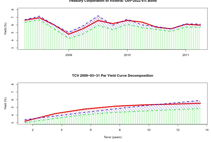
To that end, we turn now to the decomposition. Effectively, we use the surface to provide a scalar to three element vector map from each observed yield to the risk free component, credit yield premia and liquidity yield premia associated or priced into that yield. Of course, this triples the result set from our sample size to 5,823 yield components. Thus, for the sake of brevity, we illustrate the decomposition for a cross section and time series of yields for a selected issuer, namely the Treasury Corporation of Victoria (TCV).

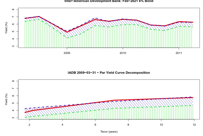
and cross sectional (yield curve) sense. As a general, rule observed yields are higher than credit yields, which in turn are greater than risk-free yields – implying positive liquidity and credit premia (in yield terms). To interpret the graph, the red lines show observed yields, and the dashed green and blue lines show the risk-free and credit yields under the decomposition, and are the par yields that correspond to pγ_it and pχi

it respectively. The vertical green

hatching shows the yield if the bond was issued by the government. The slanted blue and red hatching show the discount/premium associated with credit and liquidity risks respectively, under the zero coupon surface.

Figure 2.3: Decomposition, Treasury Corporation of Victoria yields

3

4

5

6

7

8

Treasury Corporation of Victoria: Oct−2022 6% Bond

Y

ield (%)

2009 2010 2011

2 4 6 8 10 12 14

3

4

5

6

7

8

TCV 2009−03−31 Par Yield Curve Decomposition

Tenor (years)

Y

ield (%)

this bond according to our surface and identification assumptions appeared to spike in during the GFC period around 2009, these were counterbalanced by a compression of liquidity premia (to the point where there were liquidity yield discounts) arising ostensibly from investors’ flight to quality in reaction to the stressed market condition.

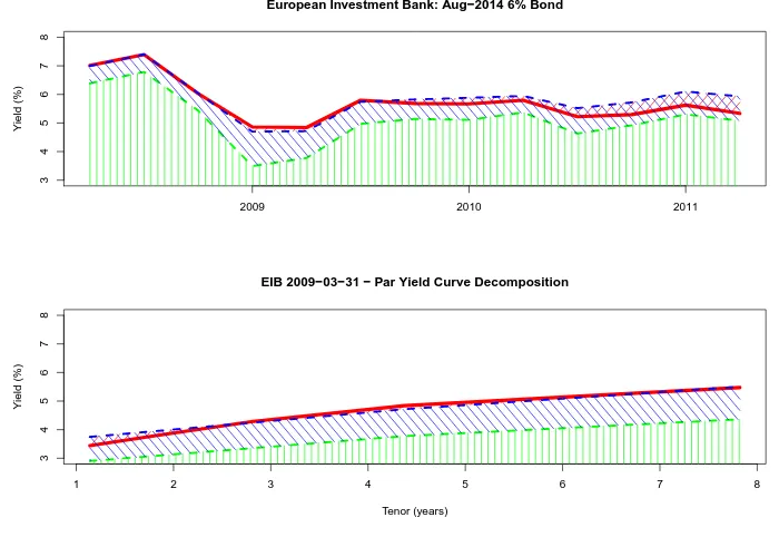
These graphs and the underlying decomposition illustrate the power and flexibility of the zero coupon surface in facilitating fixed income investment analysis. Further examples of the decomposition, for a representative suprana-tional issuer (Inter-American Development Bank, IADB), and a representative agency issuer (European Investment Bank, EIB), are set out in Figures 2.4 and 2.5. In both cases, these decompositions tell a similar story to that for TCV which we have told here.

Figure 2.4: Decomposition, Inter-American Development Bank yields

3

4

5

6

7

8

Inter−American Development Bank: Feb−2021 6% Bond

Y

ield (%)

2009 2010 2011

2 4 6 8 10 12

3

4

5

6

7

8

IADB 2009−03−31 − Par Yield Curve Decomposition

Tenor (years)

Y

ield (%)

Figure 2.5: Decomposition, European Investment Bank yields

3

4

5

6

7

8

European Investment Bank: Aug−2014 6% Bond

Y

ield (%)

2009 2010 2011

1 2 3 4 5 6 7 8

3

4

5

6

7

8

EIB 2009−03−31 − Par Yield Curve Decomposition

Tenor (years)

Y

ield (%)

way to provide evidence in support of our claims is to regress our estimates of credit premia from the zero coupon surface onto conventional determinants of credit risk, such as credit ratings and measures of financial or fiscal position. The same could be done for our liquidity premia estimates in relation to bid-ask spreads and face value on issue. The results of these regressions could then be strengthened with reference to surveys of financial market dealers and investors of Australian semi-government, supranational and agency bonds.

cross-sectional bond market pricing.

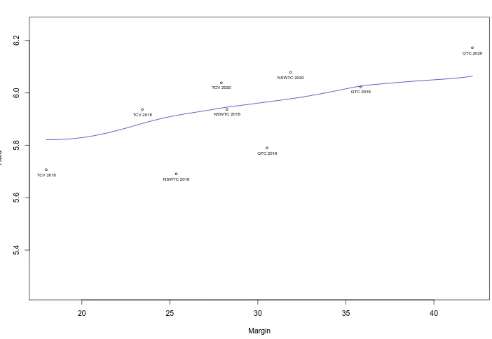
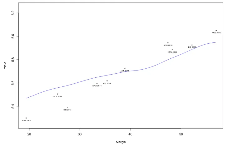
Instead, the preferable approach is therefore to explore how the zero coupon surface and the underlying market pricing is capable of accommodating a range of alternative views on credit and liquidity risk for particular bond lines and issuers’ securities. One example of how this might work is as follows: Suppose we wish to analyse a set of bonds of similar tenors, each issued by different entities that nonetheless have broadly the same credit quality. Thus, we might define our sample as all bonds of tenor between five and seven years issued by the largest State government issuers (New South Wales Treasury Corporation [NSWTC], Queensland Treasury Corporation [QTC], and TCV). Or we might consider three to five year bonds issued by the significant supranational and agency issuers (KfW, EIB and the Asian Development Bank [ADB]).

Once we have our sample, we can assume that the credit quality of these bonds is priced across the different lines according to the surface. Hence, we can use a constant slice of the surface that is perpendicular to the tenor axis and parallel to the credit margin axis (ie. the opposite direction to the decomposition presented above) to price the bonds and explore relative credit and liquidity premia.6 _{In this setup, we set the tenor constant as the average}

tenor of the bonds under consideration, as we believe that term risk has an approximately equal effect across our sample of bonds. The setup also implies that the risk-free asset swap margin will vary over a small interval that captures the margins of the bonds being examined – this allows us to control for variation in issuer credit quality.

The results of our analysis are presented in Figures 2.6 and 2.7, which show line segments of the zero coupon surface (blue lines) from 31 March 2011 for the two samples of issuers mentioned above (long semis and short supras), along with labelled points showing zero coupon yields estimated for each issuer at equivalent tenors to those of their traded bonds. The residuals between the line and the points can then be thought of as liquidity premia measured on a relative basis within the sample of bonds, since we have controlled for credit

6_{Of course, to avoid solving across segments of the surface and reconstructing the NPVs}

and term premia through our use of the zero coupon surface.

Figure 2.6: Relative pricing, long semi-government bonds

20 25 30 35 40

5.4

5.6

5.8

6.0

6.2

Margin

Y

ield

●

●

●

●

●

●

●

●

●

TCV 2016

TCV 2018

TCV 2020

QTC 2016

QTC 2018

QTC 2020

NSWTC 2016

NSWTC 2018

NSWTC 2020

Figure 2.7: Relative pricing, short supranational and agency bonds

20 30 40 50

5.4

5.6

5.8

6.0

6.2

Margin

Y

ield

●

●

●

●

●

●

●

●

●

●

ADB 2014

ADB 2015

ADB 2016

EIB 2013

EIB 2014

EIB 2015

KFW 2013

KFW 2014

KFW 2015

KFW 2016

2.4

Conclusion

We have shown that notwithstanding the effects of the Global Financial Crisis on the Australian fixed income market, the zero coupon surface summarises market pricing relatively well. This suggests that the market is pricing consistently between issuers. Further, the decomposition shows that it is possible to use the surface in more than one way to identify hitherto elusive credit and liquidity premia.

Appendix

Bootstrapping zero coupon yields The approach to bootstrapping taken here is to blend zero coupon yields from deposit instruments with those from bond

yields. As deposit instruments are already zero coupon bonds, the only calculation

necessary for deposit rates is to convert them from simple interest to continuous

compounding. In this essay, we use the cash rate and one, three and six month

overnight indexed swap rates as the yields on deposit instruments.

The rest of the zero coupon yield curve is obtained by bootstrapping and

interpolating between bond yields or swap rates. A bond of any credit quality pays

the coupon c1, . . . , cn at evenly spaced tenors t1, . . . , tn and principal of $1 at time

tn. The bond price pnis then the sum of discounted interest payments and principal,

which can be written as

pn= n

X

j=1

cjδj+δn, (2.5)

whereδj ≡e−rjtj andrj are the discount factor and zero coupon yield for tenortj.

Assume δ1, . . . , δn−1 are known. Then, by solving (2.5) for δn, the following

bootstrap relation emerges (Hagan and West, 2006):

δn =

pn−Pnj=1−1cjδj

1 +cn

⇒rn =

−1

tn

log pn−

Pn−1

j=1 cjδj

1 +cn

!

. (2.6)

The next step is to convert all quoted bond yields from their native compounding

basis into continuously compounding equivalent rates yn. The initial guesses of the

zero coupon yields rn in the bootstrap relation are given by yn. Then the dirty

price of each bond is calculated with

pn= n

X

j=1

cje−ynti+e−yntn, (2.7)

whereynis the yield to maturity of bond with tenorn. These dirty prices are treated

as the bond prices pn in the bootstrap relation (2.6). Finally, discount factors are

interpolated at all coupon dates (due to the bootstrap framework, one can use any

discount factors (Hagan and West, 2006)) and substituted into (2.6) to obtain new

estimations ofrn. This final step should be iterated, and subsequent estimates of

rn will converge rapidly onto the desired zero coupon yield curve rt∀t.

As mentioned in the text, the process described here is repeated for all issuers

in the market, to derive a complete set of zero curves for the market. While this

does not pose any problems for riskfree Government bonds, further assumptions are

required on the default and recovery processes for the framework to be successfully

applied to yields on defaultable bonds (Jarrow, 2004).

Calculating riskfree asset swap margins Formally, the riskfree asset swap margin χn is the difference between the net present value of a bonds’ cashflowscj

(where the discount factorsδj used to calculate the net present value are taken from

the risk-free zero coupon yield curve) and the traded bond price pn, expressed in

basis point terms:

χn=

Pn

j=1cjδj +δn−pn

Pn

j=1αjδj

, (2.8)

whereαj is the day count fraction applicable to period j. It is also worth noting

for those familiar with fixed income markets that risk-free asset swap margins are

related to Z-spreads (Fabozzi, 1991).

Constructing thin plate regression splines A thin plate regression spline

is an approximation to a thin plate spline, which in turn is a multivariate smoothing

spline. The outline of thin plate regression splines set out here follows closely the

original exposition in Wood (2003). In the univariate case, suppose there is a model

ri=f(xi) +i, i= 1, . . . , n, (2.9)

whereri is the response variable, f is a smooth univariate function, xi is a single

covariate and i is a mean zero error term. Smoothing splines provide a method to

estimate the smooth functionf such that it minimises the error and roughness of the fit, so that

min

f kr−f k+σ

Z

f00(x)2dx, (2.10)

wherer is a vector of ri’s, k · kis the Euclidean norm, f are the corresponding

f(xi) values, and σ is the parameter that controls the tradeoff between fit and

Thin plate splines generalise smoothing splines to include any finite number

d >1 of covariates, and allow for higher orders of differentiationmsatisfying 2m > d

in the roughness penalty (Wahba, 1990; Gu, 2002). In this case, the model becomes

ri =g(xi) +i i= 1, . . . , n,

whereg:Rd→R is an unknown multivariate smooth function to be estimated, x

is a vector of length dfromn≥dobservations andi is again a zero mean random

error term. Thin plate splines estimateg by solving the problem

min

g kr−gk+σJmd(g) (2.11)

wherer is the vector of zero coupon yieldsri, g≡(g(x1), . . . , g(xn))0 is the smooth

unknown multivariate function to be estimated, Jmd(g) is a penalty measuring

the roughness of g, and σ controls the trade off between fit and smoothness. The roughness penalty is defined in the general case as

Jmd(g) =

Z ∞ −∞ . . . Z ∞ −∞ X

ν1+...+νn=m

m!

ν1!. . . νd!

×

∂m_g

∂xν1

1 . . . ∂x

νd

d

2

dx1. . . dxd. (2.12)

and in the bivariate case (d= 2,m= 2,g=g(x1, x2)) this reduces to

J2(g) =

Z ∞

−∞

Z ∞

−∞

(g2_x1x1 + 2g_x2_1x2 +g2_x2x2)dx1dx2. (2.13)

It can be shown that the thin plate spline g which minimises (2.12) and (2.13) is characterised by the unknown parameter vectors ψ andφwhich are estimated by solving the problem

min

φ,ψ kr−Eφ−T ψk

2 _+σφ0

Eφ, (2.14)

given the n×n and n×m weighting matrices E and T (subject to T0φ = 0) (Wahba, 1990). This multivariate problem is directly comparable with the univariate

smoothing spline problem: the term within the Euclidean norm captures fitting

errors, and the quadratic form is the roughness penalty.

The thin plate spline g can be shown to be an ideal smoother in the sense that it characterises smoothness, determines the optimal tradeoff between fit and

smoothness, and finds the function that best meets this objective. On the other

are data. This means that ford >1 there areO(n2) operations for each thin plate spline fit, and implies that estimation is significantly expensive in computational

terms.

Thin plate regression splines were introduced by Simon Wood in a series of

papers (Wood, 2003, 2004, 2006, 2008; Marra and Wood, 2011) to solve the problem

with computational intractability in the estimation of thin plate splines. This is

achieved by forming a rank klow rank approximation to the parameter space and restating the thin plate spline problem with this approximation. In other words,

the basis of φis truncated to rankk, and the E matrix as it appears in the fitting error and penalty term is adjusted in a consistent manner. Parameters are then

estimated by minimising given k the worst possible changes in the fitted values and penalty induced by the approximation.7 The resulting thin plate regression spline can be shown to be an optimal approximation to the thin plate spline, that

is computationally tractable because of the low rank parameter space.

7_{In this essay, we setk= 30 when we use thin plate regression splines to fit the zero}

Chapter 3

Conditional tests of

monotonicity in term premia

3.1

Introduction

From the perspective of market participants, term premia are the essence of the Treasury yield curve.1 In the absence of term premia, investors would be indifferent between Treasury bonds of different maturities, as would the government in formulating its issuance strategy. Hence, to understand term premia is to understand the dynamics of the yield curve.

Specifically, competing theories of the yield curve can be reduced to three statements regarding term premia (Jarrow, 2010; Campbell et al., 1997). According to the expectations hypothesis, term premia are non-existent because expected returns are equal for all investment strategies in Treasury bonds. The liquidity preference hypothesis holds that term premia increase monotonically with tenor, due to investors demanding higher compensation for receiving their principal later. The preferred habitat hypothesis assumes that investors possess heterogeneous preferences across the yield curve, and that flows of funds resulting from supply and demand at different parts of the curve lead to general, non-monotonic relationships between term premia. Now, the

1_{Term premia represent the difference in expected returns from Treasury securities}

expectations hypothesis has been rejected consistently in empirical studies (Campbell and Shiller, 1991; Bekaert and Hodrick, 2001; Sarno et al., 2007), so the appropriate task for a conditional test of term structure theories is to distinguish between monotonicity and non-monotonicity in term premia, and thereby discriminate between the liquidity preference and preferred habitat hypotheses.

To choose between the competing theories, one might estimate a no-arbitrage dynamic term structure model in order to decompose Treasury yields into expectations of future monetary policy and term premia over time, and then examine the model-based term premia (Duffee, 2002; Finlay and Chambers, 2008; Wright, 2011). However, this approach is problematic because any statistical test of the term structure theories applied to model-based term premia is by definition a joint test of the model and the data. This diminishes the scope of the findings of such a test. Further, the empirical efficacy of a dynamic term structure model depends crucially on the flexibility of the functional form of the factor risk premia in the model. But these factor risk premia predetermine the model-based term premia estimates, and thus predetermine the outcome of a test for the term structure theories. Researchers have formulated increasingly flexible specifications for the factor risk premia (Cheridito et al., 2007; Joslin et al., 2010, 2011), but these suffer from a

significant loss of parsimony.

that are estimated under the condition that they be non-negative; and the Monotonicity Relations test uses the insight that expected term premia must be monotonically increasing across tenors if the minimum expected term premium (of any tenor) is positive.

When conducting inequality constraints tests, the crucial problem is the choice of the information set to be used as conditioning information. The empirical literature on excess return forecasting offers importance guidance here. It has been established that forward curve factors that are linear combinations of forward rates implied by the current yield curve can be used to forecast term premia (Cochrane and Piazzesi, 2005), which are in turn related to macroeconomic factors extracted from a panel dataset of macroeconomic variables (Ludvigson and Ng, 2009). It is therefore appropriate to characterise the conditioning information to be used in tests for monotonicity in term premia on the forward curve and macroeconomic factors.2

Accordingly, we construct conditional tests of monotonicity in term premia using information in the current yield curve and macroeconomic variables. The tests are conditional versions of the Wolak test (Boudoukh et al., 1999a) and Monotonicity Relations test (Patton and Timmermann, 2010) for monotonicity in term premia. Given that the latter paper did not implement conditional tests, and the earlier paper relied principally on an uninformative indicator variable as the conditional information set, we improve the two extant tests by using a comprehensive information set.

The results of our inequality constraints testing suggest that the use of conditioning information changes the outcome of the tests from the uncon-ditional case. Both the Monotonicity Relations and the Wolak tests suggest that U.S. Treasury bill term premia are non-monotonic when unconditional sample term premia are used. But when we condition our tests on the positive elements of the Cochrane and Piazzesi (2005) and Ludvigson and Ng (2009)

2_{In a recent paper, Duffee (2011) argues that an additional excess return forecasting}

factors, the tests suggest that the conditional term premia are monotonically increasing. The same effect is apparent, although to a lesser magnitude, when we condition on both signs of the factors. This constitutes evidence that the excess return forecasting factors do have explanatory power in respect of the conditional shape of term premia. Further, our results indicate that the conditional tests shed new light on how the monotonicity tests can be applied to term premium data, by better capturing the information that appears to influence market participants’ investment decisions when they determine U.S. Treasury bill pricing.

This essay is organised as follows. Section 3.2 discusses the conditions necessary for monotonicity in term premia to hold, in order to frame an argument for why monotonicity tests should be conditional on information from the macroeconomy and the forward curve. Section 3.3 describes the conditioning information and describes the construction of the tests. Section 3.4 applies the tests to observed U.S. Treasury bill yields. Finally, Section 3.5 concludes.

3.2

Determinants of term premia

At the outset, it is important to develop intuition around the economic forces behind the liquidity preference hypothesis. To foreshadow the discussion in this Section, the asset pricing theory identifies covariances between marginal rates of substitution as the principal driver of term premia. The literature then indicates that the current yield curve and macroeconomic variables may be of use in testing for monotonicity in term premia.

They therefore demand short tenor bonds, which drives yields lower relative to long tenor bonds, resulting in positive term premia. The opposite will hold if the covariances are greater than zero and monotonically increasing.

Economic agents’ consumption and saving decisions depend on their prefer-ences and on expected economic conditions (Varian, 1999). While preferprefer-ences are not directly observable, the asset pricing theory suggests that there is a direct link between zero coupon bond prices and average stochastic discount factors (see the Appendix). Hence, there should be information in the cur-rent yield curve about the covariances between marginal rates of substitution (Cochrane and Piazzesi, 2005). Another determinant of the covariances is economic conditions, as it is clear that the marginal rate of substitution is affected by expectations of the business cycle and real activity in the economy (Ludvigson and Ng, 2009; Hansen and Singleton, 1982). Thus, it is clear that any test for monotonicity in term premia should utilise the information in the current yield curve and the state of the macroeconomy as conditioning variables.

The forward curve factor proposed by Cochrane and Piazzesi (2005) (‘CP factor’) is an ideal candidate for use as conditioning information in tests for monotonicity in term premia, because it summarises the information in the current yield curve about expected term premia. Cochrane and Piazzesi (2005) and Kessler and Scherer (2009) experienced considerable success in regressing Treasury excess returns of various tenors onto the CP factor, but our focus will be on using the CP factor as conditioning information in the conditional monotonicity tests. Ludvigson and Ng (2009) explored the extent to which factors extracted from principal components analysis of a large panel dataset of macroeconomic variables assists in explaining term premia alongside the CP factor. The resulting economic factors (‘LN factors’) were found to contain a significant amount of additional forecasting power to the CP factor in capturing future variability in Treasury excess returns.

in the bond market include net buying pressure (Bollen and Whaley, 2004) and market flows (Vayanos and Vila, 2009), although these rely on tick level trade data, which is difficult to source in over the counter fixed income mar-kets. Additional economic influences on covariances between marginal rates of substitution include learning (Sinha, 2010), subjective expectations (Xiong and Yan, 2010), habits (Wachter, 2006) and structural breaks in the short rate process (Bulkley and Giordani, 2011). However, because these factors are unobservable and have uneven effects across term premia of different tenors, it is arguable that the clearest empirical evidence that might be found in their favour is a rejection of monotonicity in term premia.

3.3

Monotonicity tests

3.3.1

Testing framework and inputs

To fix notation and provide a formal statement of the liquidity preference hypothesis, we start by defining p(_tn) as the log riskfree zero coupon bond price. Then the riskfree zero coupon yield is y_t(n)≡ −p(_tn)/n. It follows that the log holding period return on an n period bond is given by

r_t(₊₁n) ≡p_t(₊₁n−1)−p(_tn).

The excess return rx(_tn₊₁) is the holding period return less the spot yield, and corresponds to the trade where one borrows for a single period to finance an investment in a long bond, which is unwound at the end of the period. It can be written as

rx_t(n₊₁) ≡r_t(₊₁n−1)−y_t(1).

Finally, the term premium δ(_t+1n) is the difference between adjacent excess returns, so that

δ_t(₊₁n) ≡rx_t(n₊₁) −rx(_tn₊₁−1).

as

¯

∆(i) >0, fori= 2, . . . , n.

A natural statement of the liquidity preference hypothesis in the language of statistical hypothesis testing is therefore

H0 : Any element of ¯∆≤0 HA: All elements of ¯∆>0. (3.1)

where the parameter is defined with ¯∆≡( ¯∆(2)_{, . . . ,∆¯}(n)₎0_{. These definitions}

provide the basis for the monotonicity tests and facilitate the computation of sample term premia from zero coupon yields.

Apart from sample term premia, the other input for our conditional monotonicity tests comes from the conditioning information vector Zt, which

is defined as

Zt≡ {CPˆ t,LNˆ t}.

In this expression, CPt is the Cochrane and Piazzesi (2005) forward curve

factor and LNt are the Ludvigson and Ng (2009) macroeconomic factors

(the Appendix sets out full details on how to estimate these factors). By construction, there are no restrictions on the sign of the elements of Zt.

However, the inequalities in term premia to be tested will only be preserved if the elements of the original conditioning information vectorZt are all positive.

To this end, we follow Boudoukh et al. (1993) and redefine the conditioning information Zt as

Z_t∗ ≡ {Z_t+, Z_t−}

where the filters are Z_t+ ≡ max(0, Zt) and Zt− ≡ max(0,−Zt) so that Zt

captures all possible states of the world.

The conditioning information can then be incorporated into the excess returns with the multiplication (Boudoukh et al., 1999a; Patton and Timmer-mann, 2010)

Timmermann (2010) suggested that such an approach could be taken to conducting conditional monotonicity tests, but did not actually perform conditional tests. Boudoukh et al. (1999a) did use an approach akin to equation (3.2) to condition their tests on the slope of the yield curve, but they did not have the opportunity to incorporate the Cochrane and Piazzesi (2005) and Ludvigson and Ng (2009) factors, because these factors had not yet been proposed in the literature.

Finally, let ¯∆≡( ¯∆(1)_{, . . .∆¯}(n)₎0 _{denote the vector of term premia across}

tenors by wheren is the longest tenor in the sample. Then conditional (uncon-ditional) tests for monotonicity in term premia focus on the parameter ¯∆∗ ( ¯∆), whose constituent sample means are based on the conditional (unconditional) excess returns rx∗_t+1(n) (rx(_tn₊₁)).

3.3.2

Monotonicity Relations test

Patton and Timmermann (2010) design their “Monotonicity Relations” test around the fact that if the smallest difference in adjacent excess returns is positive, then all differences must be positive and monotonicity must hold.

H0 : ¯∆≤0 HA: min i=2,...,n

¯

∆>0, (3.3)

where the minimum is taken on a piecewise basis across the conditional expected values of the parameter ¯∆.3 The distribution of the test statistic, which is the smallest average adjacent difference in excess returns, is obtained with the stationary bootstrap of Politis and Romano (1994) (see Appendix).

3.3.3

Wolak test

The Wolak test is stated in different terms to the Monotonicity Relations test. Instead of treating monotonicity as an alternative, the Wolak test posits weak monotonicity under the null and sets an unrestricted alternative (Wolak,

3_{Romano and Wolf (2011) argue that this specification of the null hypothesis misses the}

1989), so that

H0 : ¯∆≥0 HA: ¯∆ unrestricted. (3.4)

The intuition behind the Wolak test is that if the sample term premia are “close” in a statistical sense to artificial nonnegative term premia obtained from the same sample, then the liquidity preference hypothesis must hold (Boudoukh et al., 1999a). Again, full details are provided in the Appendix.

3.4

Monotonicity in U.S. term premia

In this Section, we apply the testing framework set out in the previous Section, and implement the conditional tests for monotonicity in term premia on U.S. Treasury bill excess returns conditional on the excess return forecasting factors.4 Following Patton and Timmermann (2010) and Boudoukh et al. (1999a), sample term premia are calculated with U.S. Treasury bill zero

coupon yields (tenors from two to eleven months) from the CRSP Fama–Bliss bond files dataset.5 _{This dataset is most amenable to our study because there}

is a long sample of historical data available. The series for the forward curve factor and the macroeconomic factors are sourced from the respective authors’ websites.6 _{All zero coupon yield data and conditioning information factors}

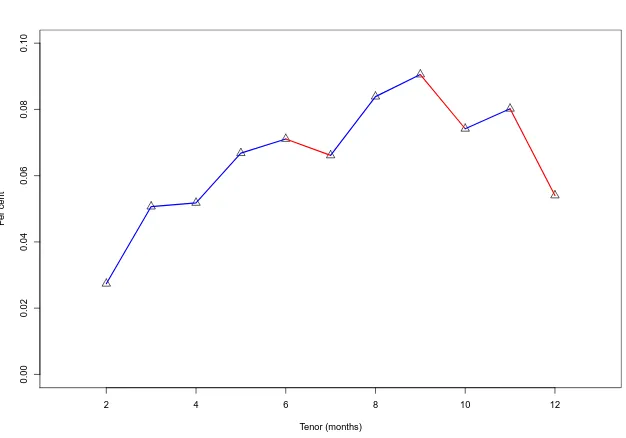
are sampled monthly, from January 1965 to December 2001, for a total of 420 observations. We use this sample period, with these particular start and end points, in order to align our sample with Patton and Timmermann (2010) (and the sample of the seminal Cochrane and Piazzesi (2005) paper), so that as far as possible our results are directly comparable. The sample mean term premia, which form the basis for our tests, are depicted in Figure 3.1.

This Figure shows that sample mean term premia are not monotonically

4_{Thanks to Andrew Patton (Duke) for MATLAB code to perform unconditional Wolak}

and Monotonicity Relation tests, which is available on his website. We have adapted this code to perform the conditional tests and compute empirical power.

5_{The zero coupon Treasury bond yield dataset available on the Federal Reserve Board}

website is an alternative source of data, and encompasses longer tenors than the Fama–Bliss dataset.

6_{Thanks to Monika Piazzesi (Stanford), Sydney Ludvigson (NYU) respectively for making}

Figure 3.1: Sample mean term premia

2 4 6 8 10 12

0.00

0.02

0.04

0.06

0.08

0.10

Tenor (months)

P

er cent

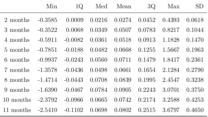
Table 3.1: Descriptive statistics, sample term premia (per cent)

Min 1Q Med Mean 3Q Max SD

2 months -0.3585 0.0009 0.0216 0.0274 0.0452 0.4393 0.0618

3 months -0.3522 0.0068 0.0349 0.0507 0.0783 0.8217 0.1044

4 months -0.5911 -0.0082 0.0361 0.0518 0.0913 1.1828 0.1470

5 months -0.7851 -0.0188 0.0482 0.0668 0.1255 1.5667 0.1963

6 months -0.9937 -0.0243 0.0560 0.0711 0.1479 1.8417 0.2361

7 months -1.3578 -0.0436 0.0498 0.0661 0.1654 2.1284 0.2790

8 months -1.4714 -0.0443 0.0708 0.0839 0.1995 2.4547 0.3238

9 months -1.6390 -0.0467 0.0784 0.0905 0.2243 3.0701 0.3750

10 months -2.3792 -0.0966 0.0665 0.0742 0.2174 3.2588 0.4253

11 months -2.5410 -0.1102 0.0698 0.0802 0.2515 3.6797 0.4650

consistent with these sample moments.

It is also important to recall that the unconditional sample means could change if they reflected conditioning information. As suggested in Section 3.2, one potential determinant of term premia dynamics could be the excess return forecasting factors. These factors therefore provide an ideal source of conditioning information for the monotonicity tests. In fact, the factors are correlated with the term premia data, and this relationship (along with the weight of the literature) suggests that they could play a role in conditional tests of monotonicity. Table 3.2 sets out the correlation matrix.

Table 3.2: Correlation matrix: excess returns and factors

CP LN CP LN

2 months -0.0197 0.2212 7 months 0.0901 0.2445

3 months 0.0117 0.2898 8 months 0.1009 0.2485

4 months 0.0610 0.2619 9 months 0.1017 0.2357

5 months 0.0890 0.2535 10 months 0.1336 0.2384

6 months 0.0960 0.2434 11 months 0.1192 0.2178

by) the unconditional sample means in each case.7 _{Figure 3.2 suggests that,}

consistent with the excess return forecasting literature, the factors appear to exert considerable influence on term premia. This provides strong impetus for the need to conduct conditional tests of monotonicity based on these factors.

Figure 3.2: Sample mean conditional term premia

2 4 6 8 10 12

0.00

0.05

0.10

0.15

0.20

0.25

Tenor (months)

P

er cent

Unconditional CP+ CP− LN+ LN−

7_{Of course, when one considers the sample average of a single signed factor, one can just}

Turning now to the central results of our analysis, Table 3.3 sets outp-values for the unconditional and conditional monotonicity tests. The unconditional tests are the same as the ones conducted in Patton and Timmermann (2010) (but for our slightly different sample end points). The conditional tests are defined by which factor is used, for instance the factor “CP+” uses the positive CP factors as conditioning information; and the factor “CP” comprises both the CP+ _{and CP}− _{factors. As there are eight LN factors (that correspond to}

the first eight principal components of their macro panel dataset), we have only used the first LN factor. The Table provides compelling evidence that the acceptance or rejection of monotonicity by each test is influenced strongly by the use of conditioning information.

Table 3.3: Monotonicity testp-values, by conditioning factor

None CP CP+ _CP− _{LN LN}+ _LN−

Top less bottom 0.0532 -0.3100 0.1718 -0.0114 -0.0187 0.0925 -0.0032

t-test (tstat) 2.4873 -0.5710 2.7502 -0.2239 1.7701 2.6824 -0.4287

t-test (p-val) 0.0064 0.7160 0.0030 0.5886 0.9616 0.0037 0.6659

MR (p-val) 0.9540 0.9130 0.1830 0.9310 0.9880 0.0040 0.9950

Wolak (p-val) 0.0465 0.0000 0.8228 0.0663 0.0001 0.8300 0.0000

Bonferonni (p-val) 0.0206 0.0450 1.0000 0.0665 0.0023 1.0000 0.0011

When we consider the results of the conditional tests that use both signs (the full factors, CP and LN), both the Wolak test and the MR test p

-values indicate that term premia do not increase monotonically across tenors. Interestingly, the strength of the unconditional tests’ outcomes is magnified in the conditional case. That is, the p-values indicate more or less significance for the outcome each test respectively when conditioning on CP or on LN relative to the unconditional case. This constitutes an initial indication that conditioning on the factors affects the outcome of the test.

To push our analysis further, we have also conditioned on the signed components of each factor separately.8 _{This enables us to study the impact of}