A code to Make Your Own Synthetic ObservaTIonS (MYOSOTIS)

A code to Make Your Own Synthetic ObservaTIonS (MYOSOTIS)

Zeinab Khorrami ,

Pouria Khalaj ,

Anne S. M. Buckner,

Paul C. Clark,

Estelle Moraux,

Stuart Lumsden,

Isabelle Joncour,

Ren´e D. Oudmaijer,

Ignacio de la Calle,

Jos´e M. Herrera-Fernandez,

Fr´ed´erique Motte,

Jos´e Manuel Blanco

and Luis Valero-Martin

3_{School of Physics and Astronomy, University of Leeds, Leeds LS2 9JT, UK} 4_{Department of Astronomy, University of Maryland, College Park, MD 20742, USA}

5_{Quasar Science Resources, S.L., Edificio Ceudas, Ctra. de La Coru˜na, Km 22.300, E-28232 Las Rozas de Madrid, Madrid, Spain}

Accepted 2019 February 13. Received 2019 February 13; in original form 2018 February 26

A B S T R A C T

We introduce our new codeMYOSOTIS(Make Your Own Synthetic ObservaTIonS) which is designed to produce synthetic observations from simulated clusters. The code can synthesize observations from both ground- and spaced-based observatories, for a range of different filters, observational conditions and angular/spectral resolution. In this paper, we highlight some of the features ofMYOSOTIS, creating synthetic observations from young massive star clusters. Our model clusters are simulated usingNBODY6 code and have different total masses, half-mass radii, and binary fractions. The synthetic observations are made at the age of 2 Myr with Solar metallicity and under different extinction conditions. For each cluster, we create synthetic images of theHubble Space Telescope(HST) in the visible (WFPC2/F555W) as well as Very Large Telescopes in the nearIR (SPHERE/IRDIS/Ks). We show howMYOSOTIScan be used to look at mass function (MF) determinations. For this aim we re-estimate stellar masses using a photometric analysis on the synthetic images. The synthetic MF slopes are compared to their actual values. Our photometric analysis demonstrate that depending on the adopted filter, extinction, angular resolution, and pixel sampling of the instruments, the power-law index of the underlying MFs can be shallower than the observed ones by at least±0.25 dex which is in agreement with the observed discrepancies reported in the literature, specially for young star clusters.

Key words: instrumentation: adaptive optics – instrumentation: high angular resolution –

techniques: photometric – telescopes – stars: luminosity function, mass function – open clus-ters and associations: general.

1 I N T R O D U C T I O N

We have been usingN-body models to study the physics of star clusters since Van Albada (van Albada 1968). Such simulations have been used to look at stellar cluster core oscillations (Giersz & Heggie2009; Heggie & Giersz2009; Hurley & Shara2012), stellar collisions (Chatterjee, Fregeau & Rasio 2009), merging of star clusters (Priyatikanto et al.2016), the evolution of multiple systems (Hurley, Tout & Pols2002) and substructures (Allison et al.2009), and the phenomenon of mass segregation and its role in cluster evolution (e.g. Portegies Zwart, McMillan & Gieles2010). Through

_{E-mail:[email protected](ZK); [email protected](PK)}

this work, the community has built up a picture of how clusters evolve (e.g. Kalirai & Richer2010), and how this may affect the initial mass function (IMF; e.g. Kroupa2001). They have also been used to place constraints on the star formation process (e.g. Parker & Reggiani2013) and how cluster dynamics can affect the stability of planetary systems (e.g. Cai et al.2017).

The results from N-body modelling have been used to help interpret the results from observational studies. For example the evolution of mass function (MF) slope in globular clusters (Baum-gardt, De Marchi & Kroupa2008), relation between the MF slope and the core radius of the star cluster (De Marchi, Paresce & Pulone 2007), and the debate on the observed mass-segregation (primordial, dynamical or observational bias) and its origin in star

2019 The Author(s)

(ii) YSCs are immersed in their natal cloud (Lada & Lada2003; Portegies Zwart et al.2010) meaning that stellar members suffer from extinction which varies from point to point. This means that applying a constant value of extinction to the entire stellar population inside the cluster leads to an incorrect estimation of stellar masses, and consequently a deformed MF.

(iii) Individual members are not fully resolved for most known YSCs due to their typically large distances. This is especially important for unresolved multiple stars (e.g. binaries) which can affect the measured low- and high-mass slopes of the MF (e.g. Malkov & Zinnecker2001; Khalaj & Baumgardt2013).

Considering all the aforementioned observational difficulties, we need to observe YSCs with better angular resolutions and high contrast imaging and preferentially at longer wavelengths. Fur-thermore, numerical simulations and models of YSCs are dictated and evolve according to observations, but the comparison of the two is far from straightforward. In particular, we always need to take an intermediate step to create synthetic observations from the simulations first, and only then the comparison with the observations is sensible.

In this paper we introduce our codeMYOSOTIS(Make Your Own Synthetic ObservaTIonS), a tool for creating synthetic observational data which produces the imaging and spectroscopic data for space-and ground-based telescopes. UsingMYOSOTISone can change the angular resolution of the observing instrument, pixel sampling of the detector, extinction and the atmospheric conditions. These factors significantly affect the photometric analysis of the individual stars detected in the field of view (FOV), especially in crowded field images like star clusters.

MYOSOTISenables us to create synthetic images/spectra of tele-scopes such as the Hubble Space Telescope (HST), Very Large Telescopes (VLT), andGaia, from theN-body simulations, to be compared with real data of the aforementioned telescopes. More-over, our tool can be used with custom configurations, meaning, that it can replicate the observations of a wide variety of instruments.

MYOSOTIShas been developed as part of the StarFormMapper1

(SFM) project, which aims to study massive stars and star cluster formation using Gaia and Herschel data. To this end, we aim to examine how synthetic observations from different telescopes produce different results on the MF of YSCs, and whether it is possible to attribute the observed discrepancy in the MFs of YSCs to different observational conditions.

This paper has two main parts: (1) detailed description of how

MYOSOTISworks (Section 2) and (2) examples of the application of the code (Section 3). In the latter part we useMYOSOTISto create syntheticHST/WFPC2 and VLT/SPHERE images of YSCs in the visible (Vband) and near-IR (Ksband) fromN-body simulations.

The details of theN-body simulations are given in Section 3.1. The

1_{http://sfm.leeds.ac.uk}

This code creates synthetic imaging and spectroscopic data of space- and ground-based telescopes as well as custom (user-defined) instruments within any FOV. The stellar and interstellar medium information (position, mass, velocity, metallicity, age) should be provided by the user. The user can choose different filters from a list (seehttp://svo2.cab.inta-csic.es/theory/fps/; Rodrigo & Solano

2013; Rodrigo et al. 2012) or define a new filter, to suit the observational instrument that they want to mimic. The observing conditions, i.e. seeing, Strehl-Ratio (SR), detector’s pixel scale of a given instrument, FOV, observer’s line of sight and finally the angular resolution of the telescope can be defined in MYOSOTIS. Since most of the instruments cannot achieve their theoretical optimum resolution (∼λ/diameter), the user can also define their own resolution. The estimated flux of stellar sources spreads on the detector using a 2D point spread function (PSF) whose full width at half-maximum (FWHM) is equal to the resolution. The user can choose a Gaussian distribution or an Airy pattern for the PSF of stellar sources. The extinction can be applied on the output data, knowing the column density of the gas in front of each source. This extinction could be uniform, patchy, or taken from a full 3D smoothed particle hydrodynamics (SPH) simulation data.

2.1 Stellar evolutionary and atmosphere models

One of the input files forMYOSOTISis the information on stellar positions, velocities, masses, ages, and metallicities. For each star, according to its age, metallicity, and mass, MYOSOTIS finds the closest stellar parameters, i.e. effective temperature (Teff), surface

gravity (logg), and luminosity (logL), using the grids ofPARSEC2

evolutionary models (Bressan et al.2012; Chen et al.2014,2015; Tang et al. 2014).PARSEChas a complete theoretical library that includes the latest set of stellar phases from pre-main sequence to main sequence, covering stellar masses from 0.09 to 350 M and ages between 0.1 Myr up to 10.1 Gyr.

After finding Teff and loggfor each star,MYOSOTIS finds the

closest stellar atmosphere model that is, the full spectral en-ergy distribution (SED), that fits the given metallicity, Teff and

loggof that star. MYOSOTIS uses the grids of NEXTGEN2 atmo-sphere models for very low mass stars and brown dwarfs with 900 K< Teff<3400 K covering loggfrom 3.5 to 6.0 (Allard et al.

1997; Hauschildt, Allard & Baron 1999), and ATLAS9 KURUCZ ODFNEW/NOVER atmosphere models (Castelli, Gratton & Kurucz

1997) for 3500 K< Teff<50 000 K covering loggfrom 0.0 to 5.0 for solar metallicity.

Users can choose a specific atmosphere model for hot and massive O- and B-type stars by setting the OB treatment parameter to ‘yes’ (i.e. OBtreatment= ‘yes’). In this case, for stars with

Figure 1. The stellar parameters of the atmosphere models used inMYOSO

-TIS.

Teff>15 000 K,MYOSOTISuses the grids ofTLUSTY3atmosphere models (Hubeny & Lanz1995) for B-type (Lanz & Hubeny2007) and O-type (Lanz & Hubeny2003) stars.TLUSTYgrids, coverTeff

from 15 000 K up to 55 000 K and loggfrom 1.75 up to 4.75. Fig.1

shows the stellar parameters covered by these atmosphere models for solar metallicity. After selecting the appropriate SED for each star,MYOSOTISwill estimate the stellar flux and extinction in a given filter, according to its distance from the observer. In addition to the aforementioned models for stellar evolution and atmospheres, users can define their own customized models and any attenuating dust that has been prescribed by the user.

2.2 Bolometric corrections and extinction

To estimate the bolometric correction (BC) of stars in different filters, we used the method explained in Girardi et al. (2002), i.e. for a given filter BC is given by

BCS_λ =Mbol,−2.5 log[4π(10 pc)2σ Teff4/L]

+2.5 log λ2

λ1 λFλ10

−0.4Aλ_Sλdλ

λ2

λ1 λf 0

λSλdλ

−m0Sλ. (1)

In this equation,Mbol, =4.83 and L=3.828×1033erg s−1.4Aλ is the extinction at wavelengthλandSλ is the filter transmission curve corresponding to the interval [λ1,λ2].Fλis the stellar intrinsic spectra at wavelengthλwhich is provided by the atmosphere model for a givenTeff, loggand metallicity.f0

λ is the reference spectra of Vega at the Earth surface5 _{that produces a known apparent}

magnitudem0

Sλin different wavelengths. Vega hasV=0.034 mag

(3670 Jy forV=0), and all colours are equal to 0. For the Vega spectrum we used syntheticATLAS9 model, withTeff = 9550 K, logg=3.95, and [M/H]= −0.5 provided by Castelli et al. (1997).

2.3 Cloud column density

The column density of the cloud in front of each stellar source (uniform or patchy) can be given directly by the user orMYOSOTIS

3_{http://nova.astro.umd.edu/Tlusty2002/tlusty-frames-cloudy.html} 4_{‘Sun Fact Sheet’https://nssdc.gsfc.nasa.gov/planetary/factsheet/sunfact.ht} ml

5_{http://basti.oa-teramo.inaf.it/BASTI/MAG ML/Vega.sed}

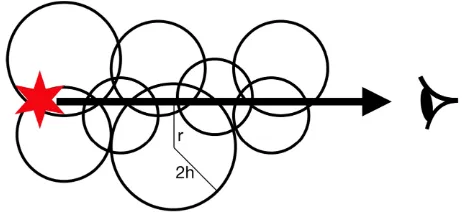
Figure 2. The cloud particles distributed in front of an stellar source. Each cloud particle has a smoothing length (h) and the column density is calculated as a function ofrfor the particles lying in the line of sight using the kernel function given in equation (2).

can calculate it using the SPH data if it is available. In the case of SPH data, the gas cloud can be located anywhere around the stellar sources as well as anywhere within the line of sight of the observer.

MYOSOTIS then calculates the cloud column density in front of each star (in the line of sight of the observer). The user should provide the cloud information (cloud particles positions, mass, and smoothing lengths). This information is the standard output of the SPH simulations. In SPH, particle properties are smoothed over a length scale,h, called the smoothing length, using a weighting function,W(r, h), called the kernel function.MYOSOTISuses M4 cubic spline kernel function (Monaghan & Lattanzio1985), shown in equation (2).

W(r/h)= 1

π h3

⎧ ⎪ ⎨ ⎪ ⎩

1−3₂(r/h)2₊3 4(r/h)

3 _0≤r/h≤1

1

4(2−r/h)

3 _1≤r/h≤2

0 2≤r/h

. (2)

Fig. 2 is a schematic representation of the cloud particles distributed in front of a stellar source.MYOSOTISdetects the cloud particles which are located in the line of sight of the observer and the stellar source. Each cloud particle has a smoothing length and a mass. The column density of the cloud can be calculated using the kernel function (equation 2), as a function of distance from the centre of each cloud particle and its mass. After estimating the column density in front of each star, we use the relation between optical extinction (AV) and hydrogen column densityNH [cm−2]

from G¨uver & ¨Ozel (2009), i.e.

NH(cm−2)=(2.21±0.09)×1021AV( mag). (3)

2.4 Extinction

The extinction for each stellar source can be calculated using two different methods:

(i)Fmodel: The code uses a function to calculate extinction in a given wavelength knowing optical extinction values (AVand RV). This function uses the average extinction curve in the optical-through-IR range (0.125–3.333μm) which is reproduced with a cubic spline and a set of anchor points from Fitzpatrick (1999).

(ii)Dmodel: The code uses synthetic extinction curves6 _from

Draine (2003a,b,c), Li & Draine (2001), and Weingartner & Draine (2001). Extinction, absorption, albedo, cos(θ), and cos2_(θ)

have been calculated for wavelengths from 1 cm (30 GHz) to 1 Å (12.4 keV), for selected mixtures of carbonaceous grains and

6_{www.astro.princeton.edu/ draine/dust/dustmix.html}

TIS needs to know the pixel-scale and the angular resolution of the observing instrument. If the telescope is ground-based (Adaptiveoptics= ‘yes’), then the user should also provide the atmospheric conditions, e.g. SR and the seeing values. If the ground-based telescope does not have any adaptive optics and its optimum resolution is poorer than seeing, user can simply choose an angular resolution equal to the seeing. The distance to the centre of mass of the object (e.g. star cluster) and the FOV should be also provided by the user. Note that all stars will not have the same distance from the observer asMYOSOTIScalculates the exact distance of each star, according to its 3D position. It is also possible to change the orientation of the object according to the observer’s line of sight. Our tool can apply the Doppler shift on the spectra of each star, according to its 3D velocity. Moreover, one can chose different values of signal-to-noise ratio (SNR) for the faintest star in the FOV. In this caseMYOSOTISwill provide an extraFITSimage with noise.

3 A P P L I C AT I O N S

To show some of the basic applications ofMYOSOTIS, we simulated four star clusters using the publicly available codeNBODY6 (Aarseth

1999). The initial conditions for these simulations are given in the following section. We generated synthetic observational data from these star clusters, usingMYOSOTIS. Then we analyse these data step by step using standard photometric methods to:

(1) extract stellar sources in each image

(2) find common stars between the data sets in different wave-lengths

(3) fit isochrones to the CMD in order to estimate the age of the star cluster

(4) estimate stellar masses in different filters in a given age (5) apply artificial stellar source recovery tests, to estimate the completeness as a function of stellar mass

(6) plot mass functions and find the derived slope of the IMF in our synthetic images

For one of our simulations (Sim5), we embedded the stars within a cloud of SPH particles, to demonstrate the ability ofMYOSOTIS

to treat patchy extinction. Details of the cloud are given below in Section 3.2.

For one of our simulations (Sim1) we also show a small region from the centre of cluster, and compare the true positions of the stars with those derived from the photometry. In addition, we use this region to show howMYOSOTIScan be used to investigate blending in stellar spectra.

3.1 N-body simulations of star clusters

We useNBODY6 to simulate the dynamical and stellar evolution of four different clusters. The clusters are set up usingMCLUSTER

Sim4 10 0.8 30

Sim5 (Sim1+gas) 104 _{0.5 0}

(Kupper et al.2011). Table1summarizes the initial conditions of the simulated clusters. As shown in the table, the simulated clusters differ in total initial mass (104_{and 10}5_M

), half-mass radius (0.5 and 0.8 pc), and binary fraction (0, 30, and 50 per cent). We have used a Plummer model (Plummer1911) for the initial mass density profile of these clusters. The IMF of stellar populations are taken from the distribution given by Kroupa (2001), with a mass range of 0.1–150 M.

The clusters are initially in virial equilibrium and there is no initial mass segregation.

For simulations with an initial binary population, the adopted algorithm (inMCLUSTER) for the pairing of primary and secondary components is as follows. The stars, with a Kroupa (2001) IMF, are split into two mass ranges by introducing a mass threshold of 5.0 M. Stars whose mass is below or above this threshold are only paired randomly with stars which belong to the same mass range. This is in rough agreement with the findings of Kobulnicky & Fryer (2007). The period distribution of binaries for the low-mass population (m <5.0 M) was obtained using the period distribution of Kroupa (1995), and for massive stars (m >5.0 M) it is based on the distribution reported by Sana & Evans (2011). The semimajor axis distribution is obtained from the aforementioned period distributions. The eccentricity (e) for low-mass binaries is drawn from a thermal eccentricity distribution, i.e.f(e)=2e(e.g. Duquennoy & Mayor1991; see also Kroupa2008), whereas for the high-mass binaries it is from the Sana & Evans (2011) eccentricity distribution.

3.2 Generating synthetic images

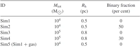
For each simulated cluster we took one snapshot of theN-body sim-ulations at the age of 2 Myr and created the synthetic observations usingMYOSOTIS. The clusters are located at the distance of R136 in the large magellanic cloud (LMC, 50 kpc from Pietrzy´nski et al.

2013). Although R136 has a metallicity index of [M/H]= −0.5 as appropriate for LMC (Dufour1984), we adopt a Solar metallicity for all simulated clusters, as the current version of MYOSOTISis limited to only Solar metallicities at present.7_{However, this will}

not affect our results since for the analysis of the photometric data we use the same metallicity that we use for the generation of the synthetic images. Thus, the general trend of our results (flattening of the observed MF; see Section 3.3) will not change as a function of metallicity.

The synthetic images have an FOV of 16 arcsec × 16 arcsec which corresponds to 4 pc×4 pc. All HST/WFPC2 images have a pixel scale of 50 mas and an angular resolution of 110 mas in

Figure 3. Synthetic images created from anN-body simulation (Sim1 in Table1) at the age of 2 Myr. Top: VLT/SPHERE/IRDIS image in nearIR (Ks) with SR=0.75 and seeing=0.8 arcsec. Bottom:HST/WFPC2 in visible (F555W). The FOV of images is 16 arcsec×16 arcsec, covering 4 pc×4 pc.

the visible (F555Wfilter). For VLT, we simulated SPHERE/IRDIS images in the nearIR (Ks) with a pixel sampling of 12.25 mas and an

angular resolution of 64 mas. For the atmospheric models of O- and B-type stars in the FOV, we have chosen the OB treatment option (see Section 2) inMYOSOTIS. For VLT images, we considered the atmospheric condition, SR to be 0.75 and a seeing halo of 0.8 arcsec. In all the images we applied the shot noise of the sky such that the SNR is 2 for the faintest star in the FOV. Fig.3shows the simulated images of Sim1 in the nearIR, IRDIS/Ks(top) and in the visible,

WFPC2/F555W(bottom).

For simulations Sim1 to Sim4 we did not consider any extinction, meaning, that there is no gas nor dust in the line of sight connecting the observer to the stars. This enables us to examine the sole effect

Figure 4. The histogram of extinction (AV) in front of each stellar sources in Sim5 simulation. See Table1for the initial conditions of the simulations. of angular resolution on the MF without being concerned about extinction. Sim5 cluster is embedded in its natal cloud which is homogeneous. The centre of the cloud is located in the centre of the cluster. We generated the cloud using the SPH codeGANDALF

(Hubber & Rosotti 2016; Hubber, Rosotti & Booth2018). The cloud contains 105_{SPH particles with smoothing lengths estimated}

byGANDALF. The total mass of the cloud is 4×103_M

which is ∼40 per cent of the total mass of the star cluster. Fig.4shows the histogram of the extinction in front of each stellar source in Sim5. The average value ofAVis 3.5 but depending on the position of the stars in the cloud it varies between 0.2 and 5.8 mag. This value ofAV is small compare to theAVof the Galactic YSCs. As an example, NGC 3603 has measuredAV ∼ 4.5 (Khorrami et al.2016) and Westerlund 1 hasAV∼11.4 (Damineli et al.2016). See Sections 2.4 and 2.3 for more information on howMYOSOTISestimates column density and extinction in front of each star, using the mass and smoothing length of cloud particles provided byGANDALF.

3.3 Photometric analysis and MF determination

We used STARFINDER(Diolaiti et al. 2000) to extract the stellar sources from the synthetic images.STARFINDERis a suitable code for the deep analysis of stellar fields, designed for AO images with high and low SR. The threshold for the photometry in our analysis was chosen to be 4σ above the sky noise. The minimum value of correlation between an acceptable stellar source and the input PSF was chosen to be 0.5 (see section 3.4 in Diolaiti et al.

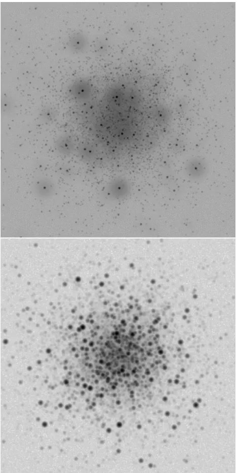
2000for more information). Table2shows the number of extracted sources and also the lowest mass estimated from the photometry

(mlow-obs) on the synthetic images. Note that the noise of the sky

has a different value in each synthetic image. As an example Sim1, Sim2 and Sim5 have same initial mass and the true number of stars in the image regions is about the same. However, a larger number of sources is extracted from Sim5 since its images have lower sky noise. Last column in Table 2shows the SNR value for a 1 M star in each synthetic image. VLT/Ks images have

higher angular resolution and better pixel-sampling than HST/V, and so more sources are detected in the VLT/Ksimages compare

to theHST/V images. The last two columns in Table2show the fraction of detected sources from the photometry versus both the real number of stars used to make the image (fourth column) and also the stars more massive thanmlow-obs(fifth column). In all cases, less

than 47 per cent of stars above the photometric threshold could be

−0.10

Sim2/VLT/Ks 3268 0.33+₋00..2010 0.207 0.460 12.46

Sim2/HST/V 1433 0.33+₋₀0_..11₀₉ 0.091 0.202 74.47

Sim3/VLT/Ks 9842 0.68+₋00..1503 0.102 0.357 8.07

Sim3/HST/V 3558 0.53+₋₀0_..12₀₀ 0.037 0.093 26.18

Sim4/VLT/Ks 10007 0.68+₋00..1503 0.102 0.351 8.07

Sim4/HST/V 3586 0.55+₋₀0_..10₀₂ 0.037 0.095 26.18

Sim5/VLT/Ks 3746 0.16+₋00..5501 0.245 0.320 25.95

Sim5/HST/V 2119 0.12+₋₀1_..05₀₁ 0.138 0.150 905.48

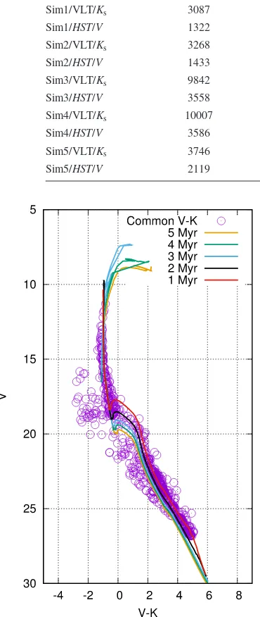
Figure 5. Colour magnitude diagram of Sim1 withinHST/F555Wand IRDIS/Ks filters. Violet circles show the common sources (747) detected between two images. Solid lines are thePARSECisochrones at different ages.

detected from the photometry. For one of the simulations (Sim1) we found the common sources between two sets of data inHST/F555W and IRDIS/Ksfilters. Fig.5shows the colour magnitude diagram

(CMD) for these common sources. Among 3087 detected sources in Ksand 1322 inF555W, we could find 747 common sources. Solid

lines in this figure are thePARSECisochrones at 1, 2, 3, 4, and 5 Myr. The 2 Myr isochrone fits well with the CMD of the observed data. The conjunction of pre-main-sequence and main-sequence stars is

Table 3. MF slope () given in equation (4) for the simulated clusters.real: MF slopes derived directly fromN-body simulations.Ks,V: MF slopes

from the photometric analysis on the synthetic images of SPHERE/IRDIS/Ks andHST/WFPC2/F555W, respectively. The low-mass limit for MF fitting is 2 MandCis the completeness value at this limit. The MF slopes are corrected for completeness and fitted with expected errors due to Poisson noise.

ID real Ks

C(per

cent) V

C(per cent) Sim1 −1.29±0.04 −1.13±0.08 96 −0.95±0.10 88 Sim2 −1.30±0.05 −1.17±0.05 95 −0.93±0.08 94 Sim3 −1.29±0.03 −0.98±0.03 74 −0.82±0.04 56 Sim4 −1.32±0.02 −1.04±0.04 75 −0.86±0.04 63 Sim5 −1.29±0.04 −1.09±0.07 96 −0.59±0.05 87

the best area to fit the isochrone, for YSCs which does not have horizontal branches (from evolved stars) at the upper part of the CMD.

We used PARSEC isochrone at 2 Myr to estimate the stellar masses. We considered a photometric error ofσmag=0.2 mag on the apparent magnitude of the detected sources. This corresponds to the average flux error of the extracted sources and provides us with an error on the stellar masses (σm). The uncertainty in the

mass of each star was accounted for when constructing the MF. We estimated the slope of the MF () defined by equation (4),

log10(N)=log10 m

M

+constant. (4)

where m is the stellar mass and N is the number of stars. We used an implementation of the non-linear least-squares Marquardt– Levenberg algorithm to calculate the value offor each cluster.

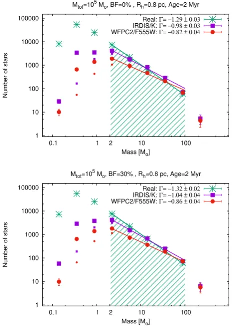
Figure 6. MF of Sim1 (top) and Sim2 (bottom) simulations, shown in Table1at the age of 2 Myr. Green is the MF derived directly fromN -body simulations. Violet and red are the MF derived from the photometric analysis of the synthetic images created in SPHERE/IRDIS/Ks filter and HST/WFPC2/F555Wfilter, respectively. Both clusters are non-segregated with initial total mass of 104M and a half-mass radius of 0.5 pc. Top has no initial binaries and bottom has 50 per cent initial binaries. Small circles/squares are the number of detected sources and large circles/squares are their completeness-corrected values. Green filled area shows the mass range where MF is fitted.

MF slopes comparison. The completeness is above 50 per cent at this limit in all the images. The high-mass limit for the MF fitting is the last point where there is a star in the underlying MF. Figs6–8

illustrate the MFs of all the simulated clusters. Small circles/squares are the observed number of stars and large circles/squares are their completeness-corrected values. Green filled area shows the mass range where MF is fitted. One can see that the measured MFs of the simulated clusters is lower (higher) than their underlying MFs at the low-mass (high-mass) end. This is due to the fact that, at low resolution the observed flux of some of the low-mass stars falls below the detection threshold, leading to an underestimation of low-mass stars. In addition, stars which are close to each other will be counted as one for a low resolution (crowding effect), leading to an overestimation of more massive objects.

Table 3 shows the MF slopes derived directly from N-body simulations (real) and also from the photometry of the synthetic images (Ks and V). The MF slopes of the clusters estimated

from the synthetic images with low resolution (HST/F555W) are flatter than those with a higher resolution (SPHERE/IRDIS/Ks) as

well as the underlying MFs derived from theN-body simulations. As explained earlier, this is due to the fact that we underestimate

Figure 7. Same as Fig.6but for Sim3 (top) and Sim4 (bottom). Both clusters are non-segregated with an initial total mass of 105_M

and a half-mass radius of 0.8 pc. Top has no initial binaries and bottom has 30 per cent initial binaries.

Figure 8. Same as Fig.6but for Sim5. The cluster is non-segregated with an initial total mass of 104_M

and a half-mass radius of 0.5 pc and no initial binaries. This cluster contains gas with the average extinction ofAV=3.5. (overestimate) the number of low-mass (high-mass) stars as a result of low resolution. Therefore, as observational conditions become poorer, the observed MF becomes flatter, mimicking mass-segregation.

Sim5 is embedded in a homogeneous cloud and has a variable extinction (see Fig. 4) throughout the cloud as each star has a different distance from the observer. In the photometric analysis of the real observational data from star clusters, the extinction

them overluminous (underluminous) and thus more (less) massive, explaining the very different shape of the MF for sim5. Given the fact that Sim5 has the same observational conditions as Sim1 with the addition of extinction, and that the MF slope of Sim5 is∼0.4 dex shallower than that of Sim1 in the visible, indicates that extinction has a major effect on the measured MF slopes of YSCs.

According to Table3, binaries do not affect the high-mass slope of the MF significantly. Note that the initial pairing of binary systems can affect the MF in addition to the observational biases.

3.4 Spectroscopy

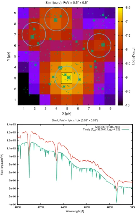
Fig.9shows the synthetic spectroscopic data produced byMYOSOTIS

from the centre of Sim1 cluster. MYOSOTIS created a cube of this region (FOV of 0.5 arcsec×0.5 arcsec) so that the spectra along each pixel is available. The image has the angular resolution of HST/WFPC2 (∼0.110 arcsec) in the HST/F450W filter and the spectroscopic resolution (λ/λ) of 700 covering wavelengths (3900−5100) Å. Creating the spectroscopic cube is computationally expensive so as an example we just created a small FOV with low spectral resolution data. The Doppler shift on the star’s spectra from their velocity were not applied (although this is a feature in

MYOSOTIS), so that we can demonstrate the effect of pure blending on the observational data.

In this small region there are 327 stars (green dots in Fig.9). 25 stars have masses above 1 M (green stars in Fig.9) and 5 of them are O- and B-type stars (green squares in Fig.9) withTeff >higher than 15 000K. The large blue circles in Fig.9shows the detected sources from the photometric analysis. Table4shows the magnitude and position (first and second columns) of B- and O-type stars in this FOV, compared to the magnitude and position derived from photometric analysis (third and fourth columns). One can see how poorly an observer can detect stellar sources. Among 327 stars just 4 of them are detected. None of the medium- and low-mass stars are detected in this region, and we have trouble detecting even the close-by massive stars.

We plotted an example of the spectra on the pixel highlighted with the black square. This is a pixel where the most massive star, in this FOV, is located (first star in Table 4). The compar-ison between low-resolution observed flux created byMYOSOTIS

and the SED of the brightest star (Teff=32500K and logg = 4.25) from TLUSTY is shown in Fig.9. This SED is chosen by

MYOSOTISaccording to the metallicity, mass and age of this star (see Section 2.1 on howMYOSOTIS chooses the proper SED for stars). The green line in Fig.9shows the SED of the brightest star observed at the distance of 50 kpc and multiplied by the chosen filter transparency.

The observed flux is higher than that of the brightest star’s intrin-sic flux, and the spectrum also has a different shape. This is because the observed flux is blended with the nearby detected sources, as well as an undetected early B-type star) and numerous undetected

Figure 9. Top: Centre of Sim1 star cluster (FoV=0.5 arcsec×0.5 arcsec).

MYOSOTIScreated a cube of this region so that the spectra along each pixel

is available. Stars with masses bellow 1 Mare shown with a small dots. 1.0–3.5 Mstars are shown with the star signs. The OB stars (Teff>15 kK) are shown with the green squares. Large blue circles shows stars detected from the photometric analysis. Bottom: shows the example of spectra along the black pixel where the most massive star in the FoV is located. Red is a low-resolution spectra created byMYOSOTISand Green is aTLUSTY

SED for the represented star at the distance of 50 kpc in HST/F450W filter.

Table 4. Magnitude and position of B- and O-type stars in Fig.9are shown in the first and second columns. The photometric magnitude and positions (large blue circles in Fig.9) are given in the third and fourth columns. magF555W X(pix),Y(pix) magphot X(pix),Y(pix) 14.8956 5.1893, 3.0490 14.894 5.000, 3.000 16.9248 3.9822, 8.3474 16.877 4.075, 8.436

18.3018 4.4093, 3.9458 – –

18.3018 8.3662, 6.0624 18.561 8.000, 6.000 18.5249 1.8390, 6.7939 18.435 1.974, 7.032

4 S U M M A RY A N D C O N C L U S I O N S

In this paper we introducedMYOSOTIS(Make Your Own Synthetic ObservaTIonS), anIDL8code written tool for simulating synthetic observation for space or ground-based telescopes which can syn-thesis both imaging and spectroscopic data.MYOSOTIScan generate the synthetic images from user input (given the position, age, and the mass of stars as well as the extinction values for the FOV) or from the output ofN-body simulations (e.g.NBODY6) as well as SPH simulations (e.g.GANDALF). It uses thePARSECevolutionary models and different atmosphere models to estimate the flux of stellar sources in different filters within a given FOV (see Section 2.1). The observing conditions, instrumental resolution and noise can be specified by the user (Section 2).MYOSOTISis a highly customizable tool, with the user being able to define their own input models, such as filters, models for stellar evolution, stellar atmospheres, etc. The

MYOSOTISlibrary of SEDs and evolutionary models can also be replaced easily to the updated models by the user. For example the high-resolution spectroscopic data from GAIA can be used as an input for different spectral type stars.

As an example of the application of MYOSOTIS in this paper, we created synthetic HST/WFPC2/F555W and VLT/SPHERE/IRDIS/Ksimages of five YSCs at the age of 2 Myr

with Solar metallicity, in the visible and nearIR. Each cluster had a different initial total mass, half-mass radius, binary fraction, and extinction. Photometry on each image was done usingSTARFINDER

package. We usedPARSECevolutionary models for re-estimating cluster’s age by isochrone fitting on the CMD. The stellar masses are re-estimated using 2 MyrPARSECisochrone and the average value of the extinction in the FOV. The underlying MF and the observed MF of each cluster (subject to different observing conditions) was derived by considering the error on stellar masses. We also performed the artificial star test on each synthetic image to estimate the completeness-corrected MF slopes (Table3). In all the cases, the slope of the MF () becomes flatter as the resolution decreases. All MF slopes of theHSTsynthetic images are flatter than those of SPHERE, which in turn are both flatter than the underlying MFs of YSCs obtained directly fromN-body simulations. Standard completeness tests do not seem to help here. This is likely because they assume that stars are randomly positioned in the stellar field, while in clusters such as those we examine here, there is significant sub-clustering (even after 2 Myr of dynamicalN-body evolution). This sub-clustering is not taken into account in the completeness tests, when randomly positioning the fake sources, and we so we tend to overestimate the completeness.

Moreover, according to our analysis, the difference between the measured MF of clusters with an initial binary population and those without binaries is≤0.1 dex, i.e. the effect of binaries on the high-mass slope of the MF is marginal. This study suggests that the observed discrepancy in the reported values of the MF slopes of YSCs (such as R136 and NGC 3603) could primarily be due to how incompleteness is treated, rather than the unresolved binary population. However significantly more work needs to be done to see whether this is indeed the case. We aim to explore this in an upcoming paper.

Our analysis also confirms that extinction can have a major effect on the measured value of the MF slopes, especially at visible band wavelengths. In particular, we demonstrated that in the presence of

8_{TheIDLversion of the source code ofMYOSOTISis publicly accessible inht} tps://github.com/zkhorrami/MYOSOTIS, and aPYTHONversion is currently under development.

extinction the measured MF slope of a YSC inHST/WFPC2/F555W images is ∼0.4 dex shallower compared to when there is no extinction (compare Sim5 with Sim1 in Table 3). The effect of resolution on both photometry and spectroscopy data can be seen in details in the example of spectrsocopic-image cube from the centre of Sim1 (Fig.9-top). Only 16 per cent (0.01 per cent) of stars with masses above 1 M (0.1 M) is detected by photometry. The spectra of a typical O-type star is blended with the nearby undetected sources (Fig.9-bottom). This result suggests that the observed mass segregation reported for some YSCs (see MF slopes reported in Eisenhauer et al. 1998; Sung & Bessell2004; Stolte et al. 2006; Harayama, Eisenhauer & Martins2008; Pang et al.

2013; Khorrami et al.2016for NGC 3603 and Malumuth & Heap

1994; Brandl et al. 1996; Hunter et al. 1996; Massey & Hunter

1998; Selman et al. 1999; Sirianni et al. 2000; Andersen et al.

2009; Khorrami et al. 2017for R136), could also be explained by observational confusion for the lack of angular resolution and unknown extinction values across the observed FOV. However more work would need to be done to support this conclusion.

In principle, the shape of MF for a given simulated cluster can be affected by binaries, multiple populations, patchy extinction, telescope limitations, and incompleteness estimates.MYOSOTIScan be used to investigate the effect of the above-mentioned parameters on the MF estimated from different observational instruments. It can also be used to explore the effects of age-determination. For example, a wrong estimation of the age of the star cluster, which can be caused by multiple stellar populations or extinction in very broad observing filters (e.g.Gaia gfilter), will also also have an effect on the derived MF.MYOSOTISis also useful for projects such as studying multiple populations in star clusters, and their affect on observationally derived parameters. This could also be used to look at cluster merger events, where each cluster has different ages and/or metallicities. The physical properties of the binary (or multiple) systems measured from synthetic observations, can be compared with their original values from the simulations.

It should be stressed that for simulating clusters with extinction,

MYOSOTIS is designed to look at the visible and near-infrared wavelengths where dust re-emission is not significant. When this approximation fails, one needs to resort to a more detailed radiative transfer approach (e.g. Koepferl, Robitaille & Dale2017).

AC K N OW L E D G E M E N T S

We would like to thank the reviewer for their constructive and insightful comments. The StarFormMapper project has received funding from the European Union’s Horizon 2020 research and innovation programme under grant agreement no. 687528. This research has made use of the SVO Filter Profile Service (http://svo2 .cab.inta-csic.es/theory/fps/) supported from the Spanish MINECO through grant AyA2014-55216. Paul C. Clark acknowledges sup-port from the Science and Technology Facilities Council (under grant ST/N00706/1). Finally, we would also like to thank Lee G. Mundy for his suggestions which led to the improvement of this work.

R E F E R E N C E S

Aarseth S. J., 1999,PASP, 111, 1333

Allard F., Hauschildt P. H., Alexander D. R., Starrfield S., 1997,ARA&A, 35, 137

Allison R. J., Goodwin S. P., Parker R. J., de Grijs R., Portegies Zwart S. F., Kouwenhoven M. B. N., 2009,ApJ, 700, L99

Chen Y., Bressan A., Girardi L., Marigo P., Kong X., Lanza A., 2015, MNRAS, 452, 1068

Chen Y., Girardi L., Bressan A., Marigo P., Barbieri M., Kong X., 2014, MNRAS, 444, 2525

Damineli A., Almeida L. A., Blum R. D., Damineli D. S. C., Navarete F., Rubinho M. S., Teodoro M., 2016,MNRAS, 463, 2653

De Marchi G., Paresce F., Pulone L., 2007,ApJ, 656, L65

Diolaiti E., Bendinelli O., Bonaccini D., Close L., Currie D., Parmeggiani G., 2000,A&AS, 147, 335

Dom´ınguez R., Fellhauer M., Bla˜na M., Farias J. P., Dabringhausen J., 2017, MNRAS, 472, 465

Draine B. T., 2003a,ARA&A, 41, 241 Draine B. T., 2003b,ApJ, 598, 1017 Draine B. T., 2003c,ApJ, 598, 1026

Dufour R. J., 1984 , in Van den Bergh S., de Boer K. S. D., eds, Proc. IAU Symp. 108, Structure and Evolution of the Magellanic Clouds. Reidel, Dordrecht, p. 353

Duquennoy A., Mayor M., 1991, A&A, 248, 485

Eisenhauer F., Quirrenbach A., Zinnecker H., Genzel R., 1998,ApJ, 498, 278

Espinoza P., Selman F. J., Melnick J., 2009,A&A, 501, 563 Fitzpatrick E. L., 1999,PASP, 111, 63

Giersz M., Heggie D. C., 2009,MNRAS, 395, 1173

Girardi L., Bertelli G., Bressan A., Chiosi C., Groenewegen M. A. T., Marigo P., Salasnich B., Weiss A., 2002, A&A, 391, 195

G¨uver T., ¨Ozel F., 2009, MNRAS, 400, 2050

Harayama Y., Eisenhauer F., Martins F., 2008,ApJ, 675, 1319 Hauschildt P. H., Allard F., Baron E., 1999,ApJ, 512, 377 Heggie D. C., Giersz M., 2009,MNRAS, 397, L46

Hubber D., Rosotti G., 2016, Astrophysics Source Code Library, record ascl:1602.015

Hubber D. A., Rosotti G. P., Booth R. A., 2018,MNRAS, 473, 1603 Hubeny I., Lanz T., 1995,ApJ, 439, 875

Hunter D. A., O’Neil E. J., Jr, Lynds R., Shaya E. J., Groth E. J., Holtzman J. A., 1996, ApJ, 459, L27

Hurley J. R., Shara M. M., 2012,MNRAS, 425, 2872 Hurley J. R., Tout C. A., Pols O. R., 2002,MNRAS, 329, 897 Kalirai J. S., Richer H. B., 2010,Phil. Trans. R. Soc. A, 368, 755

Lanz T., Hubeny I., 2003,ApJS, 147, 225 Lanz T., Hubeny I., 2007,ApJS, 169, 83 Li A., Draine B. T., 2001,ApJ, 554, 778

Malkov O., Zinnecker H., 2001,MNRAS, 321, 149 Malumuth E. M., Heap S. R., 1994,AJ, 107, 1054 Massey P., Hunter D. A., 1998,ApJ, 493, 180 Monaghan J. J., Lattanzio J. C., 1985, A&A, 149, 135

Pang X., Grebel E. K., Allison R. J., Goodwin S. P., Altmann M., Harbeck D., Moffat A. F. J., Drissen L., 2013,ApJ, 764, 73

Parker R. J., Goodwin S. P., Wright N. J., Meyer M. R., Quanz S. P., 2016, MNRAS, 459, L119

Parker R. J., Reggiani M. M., 2013,MNRAS, 432, 2378 Pietrzy´nski G. et al., 2013,Nature, 495, 76

Plummer H. C., 1911,MNRAS, 71, 460

Portegies Zwart S. F., McMillan S. L. W., Gieles M., 2010,ARA&A, 48, 431

Priyatikanto R., Kouwenhoven M. B. N., Arifyanto M. I., Wulandari H. R. T., Siregar S., 2016,MNRAS, 457, 1339

Rodrigo C., Solano E., 2013, The Filter Profile Service Access Protocol. Available at:http://ivoa.net/documents/Notes/SVOFPS/index.html Rodrigo C., Solano E., Bayo A., 2012, The SVO Filter Profile Service.

Available at:http://ivoa.net/documents/Notes/SVOFPS/index.html Sana H., Evans C. J., 2011, in Neiner C., Wade G., Meynet G., Peters G.,

eds,Proc. IAU Symp. 272, Active OB Stars: Structure, Evolution, Mass Loss, and Critical Limits, p. 474

Selman F., Melnick J., Bosch G., Terlevich R., 1999, A&A, 347, 532 Sirianni M., Nota A., Leitherer C., De Marchi G., Clampin M., 2000,ApJ,

533, 203

Stolte A., Brandner W., Brandl B., Zinnecker H., Grebel E. K., 2006,AJ, 132, 253

Sung H., Bessell M. S., 2004,AJ, 127, 1014

Tang J., Bressan A., Rosenfield P., Slemer A., Marigo P., Girardi L., Bianchi L., 2014,MNRAS, 445, 4287

van Albada T. S., 1968, Bull. Astron. Inst. Netherlands, 19, 479 Weingartner J. C., Draine B. T., 2001,ApJ, 548, 296