www.atmos-chem-phys.net/14/11221/2014/ doi:10.5194/acp-14-11221-2014
© Author(s) 2014. CC Attribution 3.0 License.
Aerosol microphysics simulations of the Mt. Pinatubo eruption with
the UM-UKCA composition-climate model
S. S. Dhomse1, K. M. Emmerson2, G. W. Mann1,3, N. Bellouin4, K. S. Carslaw1, M. P. Chipperfield1, R. Hommel5,*, N. L. Abraham3,5, P. Telford3,5, P. Braesicke3,5,**, M. Dalvi3,6, C. E. Johnson6, F. O’Connor6, O. Morgenstern7, J. A. Pyle3,5, T. Deshler8, J. M. Zawodny9, and L. W. Thomason9
1School of Earth and Environment, University of Leeds LS2 9JT, UK
2CSIRO Marine and Atmospheric Research, Aspendale, Victoria 3195, Australia 3National Centre for Atmospheric Science (NCAS-Climate), UK
4Department of Meteorology, University of Reading, Reading, UK 5Department of Chemistry, University of Cambridge, Cambridge, UK 6Met Office, Exeter, UK
7National Institute of Water and Atmospheric Research (NIWA), Lauder, New Zealand 8University of Wyoming, Wyoming, USA
9NASA Langley Research Center, Hampton, Virginia, USA *now at: IUP, University of Bremen, Bremen, Germany
**now at: IMK-ASF Karlsruhe Institute of Technology, Karlsruhe, Germany
Correspondence to: S. S. Dhomse (s.s.dhomse@leeds.ac.uk)
Received: 15 December 2013 – Published in Atmos. Chem. Phys. Discuss.: 28 January 2014 Revised: 16 September 2014 – Accepted: 16 September 2014 – Published: 24 October 2014
Abstract. We use a stratosphere–troposphere composition– climate model with interactive sulfur chemistry and aerosol microphysics, to investigate the effect of the 1991 Mount Pinatubo eruption on stratospheric aerosol properties. Satel-lite measurements indicate that shortly after the eruption, between 14 and 23 Tg of SO2 (7 to 11.5 Tg of sulfur) was present in the tropical stratosphere. Best estimates of the peak global stratospheric aerosol burden are in the range 19 to 26 Tg, or 3.7 to 6.7 Tg of sulfur assuming a composition of between 59 and 77 % H2SO4. In light of this large uncer-tainty range, we performed two main simulations with 10 and 20 Tg of SO2 injected into the tropical lower stratosphere. Simulated stratospheric aerosol properties through the 1991 to 1995 period are compared against a range of available satellite and in situ measurements. Stratospheric aerosol opti-cal depth (sAOD) and effective radius from both simulations show good qualitative agreement with the observations, with the timing of peak sAOD and decay timescale matching well with the observations in the tropics and mid-latitudes. How-ever, injecting 20 Tg gives a factor of 2 too high stratospheric aerosol mass burden compared to the satellite data, with
con-sequent strong high biases in simulated sAOD and surface area density, with the 10 Tg injection in much better agree-ment. Our model cannot explain the large fraction of the in-jected sulfur that the satellite-derived SO2and aerosol bur-dens indicate was removed within the first few months after the eruption. We suggest that either there is an additional al-ternative loss pathway for the SO2not included in our model (e.g. via accommodation into ash or ice in the volcanic cloud) or that a larger proportion of the injected sulfur was removed via cross-tropopause transport than in our simulations.
whereas the 10 Tg run compared best to the satellite measure-ments, a significant low bias is apparent in the coarser size channels in the volcanically perturbed lower stratosphere. Overall, our results suggest that, with appropriate calibration, aerosol microphysics models are capable of capturing the observed variation in particle size distribution in the strato-sphere across both volcanically perturbed and quiescent con-ditions. Furthermore, additional sensitivity simulations sug-gest that predictions with the models are robust to uncertain-ties in sub-grid particle formation and nucleation rates in the stratosphere.
1 Introduction
Volcanic eruptions can have significant impacts on atmo-spheric composition and climate (e.g. McCormick et al., 1995; Robock, 2000). Powerful explosive eruptions can in-ject large amounts of SO2, ash, water vapour and various other chemical species directly into the stratosphere. Vol-canic SO2 injected into the stratosphere is chemically con-verted to sulfuric acid vapour over a timescale of days to months, causing substantial new particle formation and aerosol growth by condensation. Volcanic enhancements of the stratospheric aerosol can be long lasting, with optically active particle concentrations remaining substantially en-hanced for several years in the case of tropical eruptions (Deshler et al., 2003). The perturbed stratospheric aerosol al-ters the Earth’s radiative balance with increased albedo via enhanced back-scattering of solar radiation, cooling the sur-face and increased absorption of terrestrial long-wave radi-ation, warming the stratosphere (Labitzke and McCormick, 1992). The relative magnitude of these short-wave and long-wave radiative effects are strongly influenced by the aerosol particle size distribution (Lacis et al., 1992; Hansen et al., 1992).
The long-wave radiative heating induced by the thicker aerosol layer also modifies the stratospheric circulation (e.g. Young et al., 1994), leading to indirect radiative effects via dynamical changes in ozone and meridional transport, with important implications for surface climate (Robock and Mao, 1992; Graf et al., 1993). Volcanically increased aerosol sur-face area density (SAD) can also accelerate heterogeneous chemistry perturbing stratospheric NOy species, halogens and ozone (e.g. Solomon et al., 1996). Quantifying the net impact from these direct and indirect radiative effects is very important to better understand volcanic influences within the historical climate records.
There is an increasing recognition that having a good rep-resentation of stratospheric processes is important for climate projections (e.g. Scaife et al., 2012). However, whereas most coupled atmosphere–ocean climate models (e.g. Jones et al., 2011) that carried out historical integrations for CMIP5 (Tay-lor et al., 2012) included a prognostic treatment of
tropo-spheric aerosol, stratotropo-spheric aerosols are treated separately. Some models impose volcanic forcings and heating rates (e.g. Stenchikov et al., 1998) or base these on prescribed time-varying aerosol optical depth climatologies (such as Sato et al., 1993). None of the CMIP5 climate models are able to capture the complex dynamical changes associated with large tropical eruptions (Driscoll et al., 2012). There is now an established group of composition–climate models (CCMs) which simulate stratospheric chemistry with inter-active ozone radiative effects (e.g. SPARC, 2010), but few include prognostic treatment of stratospheric aerosol. Even relatively modest changes in stratospheric aerosol can exert a significant radiative forcing (e.g. Solomon et al., 2011) and expected future changes in stratospheric circulation further motivate the need for interactive stratospheric aerosol in cli-mate models.
We use the stratosphere–troposphere composition-climate model UM-UKCA (Unified Model – UK Chemistry and Aerosol) to simulate stratospheric aerosol interactively. The model includes the GLOMAP-mode aerosol scheme and calculates aerosol optical properties online and consistently with the 3-D evolution of the particle size distribution, as driven by the underlying microphysical processes. We use the 1991 Mt Pinatubo eruption as a test case to examine simulated aerosol properties comparing to a range of satel-lite and in situ observations covering the background, vol-canic perturbation and decay periods. Pinatubo erupted in the Philippines (15.1◦N, 120.4◦E) on 15 June 1991 and was the largest tropical eruption since Krakatoa 1883. Based on column SO2 mass loadings derived from ultraviolet ra-diation measurements from the Total Ozone Monitoring Spectrometer (TOMS) instrument, Bluth et al. (1992) esti-mated that the eruption injected approximately 20 Tg into the tropical stratosphere. Guo et al. (2004a) re-evaluated the post-Pinatubo TOMS data, and also analysed measurements from the Television Infra-red Observation Satellite Vertical Sounder (TOVS), finding total SO2 released to be in the range 14 to 23 Tg (7 to 11.5 Tg of sulfur).
into a peak aerosol sulfur burden uncertainty range of 3.7 to 6.7 Tg of sulfur. Taken together, these findings suggest that a large proportion of the sulfur was removed from the stratosphere within the first few months after the eruption, with potential loss pathways involving sedimentation, cross-tropopause transport out of the stratosphere (Deshler, 2008) or enhanced removal via interactions with ash or ice in the Pinatubo cloud (Guo et al., 2004b). Monthly balloon sound-ings of total and size-resolved particle concentrations carried out at Laramie, Wyoming (e.g. Deshler, 1994) showed that although substantially enhanced particle concentrations were detected in the lowermost stratosphere by mid-July, the main part of the volcanic plume was only transported to NH mid-latitudes several months later.
There have been many previous global modelling stud-ies to investigate the evolution of the stratospheric aerosol following the Pinatubo eruption. However, most have used aerosol schemes that simulate only the evolution of aerosol mass, prescribing a fixed particle size distribution for sedi-mentation and radiative effects (e.g. Timmreck et al., 1999; Oman et al., 2006; Aquila et al., 2012). However, size-resolved stratospheric aerosol modules which include micro-physical processes such as new particle formation, coagula-tion and condensacoagula-tion have also been developed. The first Pinatubo aerosol microphysics simulations were carried out in 2-D models (Bekki and Pyle, 1994; Weisenstein et al., 1997) with single-moment sectional schemes where mass in numerous size bins is transported. More recently, several 3-D general circulation models (GCMs) with aerosol micro-physics schemes have also been developed, to predict sedi-mentation and changes in radiative properties in conjunction with an evolving stratospheric particle size distribution (e.g. Timmreck, 2001; Toohey et al., 2011; English et al., 2012, 2013).
Although there have been this development of more so-phisticated models, most of these studies evaluated their simulations against a limited set of observational data sets, primarily aerosol optical depths (AODs) derived using Ad-vanced Very High Resolution Radiometer (AVHRR) and SAGE II measurements. Using a mass-based prognostic stratospheric aerosol module in a middle-atmosphere ver-sion of the ECHAM4 climate model, Timmreck et al. (1999) showed that the two distinct maxima in AOD apparent in AVHRR- and SAGE-II-based stratospheric aerosol optical depth (sAOD) could be simulated, but the model failed to simulate the observed slow sAOD decay in the tropics af-ter the peak. Similarly, Pitari and Mancini (2002) used a GCM coupled to a global chemistry transport model with interactive aerosol microphysics, and could simulate SH sAOD reasonable well, but NH and tropical sAOD was bi-ased low. Aquila et al. (2012) used a GCM with a mass-based aerosol scheme radiatively coupled to the model dy-namics. They found that simulated sAOD was higher than both AVHRR and SAGE II during the first few months, but showed very good agreement during the later phase. Using
a sectional aerosol microphysics module with injection alti-tude between 15.5 and 27 km, English et al. (2013) achieved good agreement with SAGE- and AVHRR-observed sAOD in NH mid-latitudes for the first 12 months after the eruption but too rapid decay in sAOD through later months. They also compared model aerosol effective radius (Reff) evolution against observations from SAGE II and in situ measurements (for e.g. Russell et al., 1996; Bauman et al., 2003), finding that peak values in the model NH tropical stratosphere oc-curred earlier than in the observations. Some of these model– observation biases in earlier studies may be linked with the transport-related issues (e.g. the lack of a quasi-biennial os-cillation, QBO) in the underlying GCM, whereas some may be linked to the simplified treatment of the particle size distri-bution. Other causes such as interactions with ash, or missing minor eruptions such as Mount Hudson in Chile (Septem-ber 1991) have also been suggested.
Although they have near-global spatial extent, satellite measurements of sAOD andReff constrain only integrated stratospheric aerosol properties over the full particle size range. Balloon-borne measurements (e.g. Deshler, 1994) en-able a closer examination of the particle size distribution, but are available at only a small number of sites.
Here, we use both satellite and balloon-borne measure-ments to evaluate the UM-UKCA simulated stratospheric aerosol properties, and seek to provide a wider set of obser-vational constraints for the models and to better understand how the stratospheric aerosol layer was perturbed. In Sect. 2 we describe the model, including the experimental set-up and the developments to the aerosol and chemistry schemes which extend its applicability to both stratospheric and tro-pospheric conditions. Section 3 describes the measurements that are used to evaluate the model. Results and discussion about potential causes of model–observation biases are pre-sented in Sect. 4 and 5, respectively. Summary and major conclusions are presented in Sect. 6.
2 Model description
In order to simulate stratospheric aerosol precursor gas phase species, we have extended the existing UM-UKCA stratospheric chemistry scheme to also include sulfur chem-istry (see Sect. 2.1). The coupling to the GLOMAP-mode aerosol microphysics module (Mann et al., 2010), and its adaptation for stratospheric conditions, is described in Sect. 2.2. Surface emissions of NOx, CO and HCHO are from the RCP 4.5 scenario. Lower boundary conditions are ap-plied for CH4, N2O, CFC-11 (CFCl3) and CFC-12 (CF2Cl2) according to WMO (2011). Heterogeneous chemical reac-tions use time-varying prescribed aerosol surface area den-sity produced for the SPARC Assessment of the Strato-spheric Aerosols Properties report (SPARC, 2006). We in-clude surface and elevated emissions of anthropogenic SO2 from Lamarque et al. (2010) with also a 3-D source from passively degassing volcanoes from Andres and Kasgnoc (1998). DMS emissions are simulated interactively using a seawater concentration climatology of Kettle and Andreae (2000) with the sea–air exchange function of Liss and Mer-livat (1986). For OCS, which has a tropospheric lifetime of about 2 years (Montzka et al., 2007), we do not include an emissions source, but instead apply a fixed lower boundary condition of 550 pptm.
2.1 Stratospheric chemistry extended to include the sulfur cycle
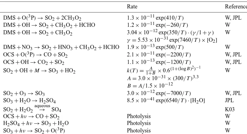
The existing UM-UKCA stratospheric chemistry scheme (Morgenstern et al., 2009) covers the oxidation of CH4and CO, with chlorine and bromine chemistry and their interac-tion with HOx, NOxand Oxcycles including heterogeneous reactions on polar stratospheric clouds (PSCs) and liquid sul-fate aerosols (Chipperfield and Pyle, 1998). Here, we have extended the scheme to also include a stratospheric aerosol precursor chemistry scheme (Weisenstein et al., 1997) with updates to reaction rates from Sander et al. (2006), see Ta-ble 1. The added chemistry includes the steady background source of SO2 from OCS, which principally maintains the stratospheric aerosol during volcanically quiescent periods (e.g. Carslaw and Kärcher, 2006). Also included are photol-ysis reactions for H2SO4and SO3, which occur above about 30 km and lead to a reservoir of SO2building up during po-lar winter, enabling new particle formation in the popo-lar lower stratosphere during spring (Mills et al., 2005). The chemistry is integrated with the ASAD chemical integration package (Carver et al., 1997) with the Newton–Raphson sparse matrix solver from Wild et al. (2000). Photolysis rates are calculated using the FAST-JX online photolysis (Neu et al., 2007) fol-lowing the implementation described in Telford et al. (2013). The cross-section of H2SO4 is assumed analogous to the cross-section of HCl (× 0.016) following the method of Bekki and Pyle (1992). Aqueous sulfate production in (tropo-spheric) liquid clouds is also passed to the GLOMAP module for growth of accumulation and coarse soluble particles.
2.2 The aerosol microphysics module adapted for the stratosphere
The GLOMAP aerosol microphysics module was initially developed as a component of the TOMCAT 3-D offline Chemical Transport Model (Chipperfield, 2006) with both 2-moment sectional (Spracklen et al., 2005) and 2-moment modal versions (Mann et al., 2010) available. The computa-tionally faster modal scheme (GLOMAP-mode) was specif-ically designed for longer integrations within UM-UKCA and applies the same aerosol microphysics representations as the sectional scheme but with the size distribution pa-rameterised into seven log-normal modes, being similar in framework to that used in ECHAM-HAM (e.g. Stier et al., 2005). The GLOMAP-mode scheme produces aerosol prop-erties in good agreement with the more sophisticated sec-tional scheme under most tropospheric conditions (Mann et al., 2012).
Since this study investigates the evolution of the strato-spheric aerosol layer after Pinatubo, we use only the four soluble modes and treat only sulfate and sea salt components – the latter included to give reasonable representation of tro-pospheric aerosol optical properties. For this work, the model approaches for water uptake, particle density, vapour conden-sation and new particle formation have been adapted to be applicable across stratospheric and tropospheric conditions. In the following sections, we briefly describe these updates.
2.2.1 Water uptake
In the standard version of GLOMAP-mode described by Mann et al. (2010), water uptake is calculated using ZSR (Zdanovskii, 1948; Stokes and Robinson, 1966), which is not applicable in stratosphere conditions. At pressures below 150 hPa we therefore instead use the expression of Carslaw et al. (1995) to provide the aerosol water content. At 225 K and 101 hPa, the composition of the solution is 74.5 % H2SO4 and 25.5 % water, approximating the 75 % weight fraction assumed in some studies (e.g. Stenchikov et al., 1998; Oman et al., 2006).
2.2.2 Particle density
As composition of the aqueous sulfuric acid solution droplets also affects their density, we modified GLOMAP-mode for the stratosphere. For pressures lower than 150 hPa, density values for each mode are replaced with values from a look-up table based on the measurements of Martin et al. (2000) as a function of the sulfuric acid weight-fraction.
2.2.3 Condensation and vapour pressure of H2SO4
Table 1. Additional sulfur chemistry reactions and rates within UM-UKCA, W=Weisenstein et al. (1997), JPL=Sander et al. (2006), K03=Kreidenweis et al. (2003).
Rate Reference
DMS+O(3P)→SO2+2CH3O2 1.3×10⁻¹¹exp(410/T ) W, JPL
DMS+OH→SO2+CH3O2+HCHO 1.2×10⁻¹¹exp(−260/T ) W
DMS+OH→SO2+CH3O2 3.04×10⁻¹²exp(350/T )·(γ /1+γ ) W
γ=5.53×10⁻³¹exp(7460/T )× [O2]
DMS+NO3→SO2+HNO3+CH3O2+HCHO 1.9×10⁻¹³exp(500/T ) W
OCS+O(3P)→CO+SO2 2.1×10⁻¹¹exp(−2200/T ) W, JPL
OCS+OH→CO2+SO2 1.1×10⁻¹³exp(−1200/T ) W, JPL
SO2+OH+M→SO3+HO2 k(T )= 1+AB×0.6
(1+(logB)2)−1
W
A=3.0×10−31×(300/T )3.3 B=A/1.5×10−12
SO2+O3→SO3 3.0×10⁻¹²exp(−7000/T ) W, JPL
SO3+H2O→H2SO4 8.5×10−41exp(6540/T )· [H2O] JPL
SO2+H2O2 aqueous
→ SO4 K03
OCS+hν→CO+SO2 Photolysis W
H2SO4+hν→SO3+H2O Photolysis W
SO3+hν→SO2+O(3P) Photolysis W
in tropospheric conditions, above ∼25–30 km, the vapour pressure of H2SO4(pH2SO4) becomes significant as the tem-perature increases in the stratosphere and above∼35 km the sulfuric acid droplets rapidly evaporate (Hamill et al., 1997; Hommel et al., 2011).
We therefore now calculate pH2SO4 online in the model following Kulmala and Laaksonen (1990) and the conden-sation rates are calculated consistently with the difference between the vapour pressure and the gas phase partial pres-sure. We also apply a simple approach to particle evaporation whereby if the ambient gas phase H2SO4partial pressure is less thanpH2SO4, the number concentration for all modes is reduced at a fast decay rate of 50 % per condensation time step, which corresponds to an e-folding timescale of around 17 min.
2.2.4 New particle formation
Previous versions of GLOMAP (e.g. Mann et al., 2010) formed new H2SO4–H2O particles based on the Kulmala et al. (1998) parameterisation for binary homogeneous nu-cleation. This is only applicable at temperatures in the range 233–298 K. Vehkamäki et al. (2002) suggested that condi-tions for nucleation are also favourable at∼200 K in the up-per tropical troposphere and they updated the Kulmala et al. (1998) parameterisation to be applicable down to lower tem-peratures and humidities. To allow GLOMAP-mode to be ap-plied in both tropospheric and stratospheric conditions, we have incorporated the Vehkamäki et al. (2002) parameteri-sation, and used it within the recommended ranges of tem-perature (190 to 305 K) and H2SO4 concentration (104 to 1011cm−3). Note that we also use the expression of
Kermi-nen and Kulmala (2002) to convert the cluster nucleation rate from Vehkamäki et al. (2002) into an “apparent nucleation rate” at 3 nm. The nucleation rate is set to zero in subsatu-rated conditions.
2.2.5 Size distribution
are received from the adjacent smaller mode, the transferred number and mass is added to that existing in the mode, with the mean size reformulated reformulated consistently with theσgvalue for the mode.
Kokkola et al. (2009) compared size distributions simu-lated by a modal and three sectional schemes in a box model. While the four models agreed well in background strato-spheric conditions, in volcanically perturbed conditions, the size distributions were found to be better represented with narrower mode widths. In particular, with the original coarse mode σg of 2.0, they found the modal scheme overpre-dicted the Reff compared to a reference sectional scheme with a large number of bins. Niemeier et al. (2009) used an improved version of the same modal microphysics scheme wherebyσgfor the accumulation soluble mode was reduced to 1.2 and the coarse mode was deactivated.
Here we are applying the modal GLOMAP scheme to vol-canically perturbed stratospheric conditions, and also using the same modes to represent tropospheric aerosol. In the tro-posphere, the coarse soluble mode in GLOMAP-mode al-most exclusively contains sea-salt, and the scheme follows Wilson et al. (2001) and Vignati et al. (2004) in using a value of 2.0 forσg in this mode, which are based on values given in D’Almeida et al. (1991).
To ensure the size distribution and vertical profile of the simulated coarse sea-salt particles is retained as evaluated in previous model versions (Mann et al., 2012), we retain the σg value of 2.0 for the coarse soluble mode. However, we now de-activate mode-merging between the accumulation and coarse soluble modes, which allows the accumulation soluble mode to continue to grow larger than 1 micron diam-eter in strongly perturbed conditions. We also retain the σg value of 1.4 for the soluble accumulation mode in GLOMAP-mode, as reduced by Mann et al. (2012) from the value of 1.59 used in Mann et al. (2010), to better compare with size distributions simulated by the sectional scheme and from ob-servations. Theσg=1.59 values for the nucleation and Aitken modes are also retained.
2.3 Experimental setup
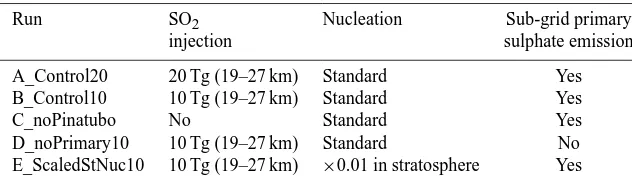
For this study, we carried out several 5-year model integra-tions, as summarised in Table 2. In addition to a background run (C_noPinatubo) without any Pinatubo emission, two ref-erence simulations were carried out with 20 (A_Control20) and 10 Tg (B_Control10) of SO2 injected into the tropical stratosphere on 15 June 1991 between 19 and 27 km. To en-sure we closely match the initial spatial distribution of the aerosol cloud, we inject the SO2across the eight model grid boxes between 0–20◦N along 120.5◦E. We emit 3 % of the SO2 mass from Pinatubo directly as sulfuric acid particles (assumed to form at the sub-grid scale) with half emitted with assumed geometric mean radius of 15 and 40 nm as in Spracklen et al. (2005). For all the simulations the entire set of tracers were initialised from fields after 8 years spin-up.
The spin-up run started from zero aerosol and gas phase sul-fur species, with other gases initialised from the UM-UKCA REF-C1 integration from the SPARC Lifetimes of Strato-spheric Ozone-Depleting Substances, Their Replacements, and Related Species report (SPARC, 2013), representative of 1990 conditions.
To assess the robustness of the model to uncertainties in particle formation processes, which are known to be consid-erable uncertain in the stratosphere, we also carried out two sensitivity simulations with are as run B_Control10, but we switch off the sub-grid particle source (primary sulfate emis-sion) from Pinatubo (D_noPrimary10) and reduce the nucle-ation rate (E_ScaledStNuc10) in the stratosphere by a factor of 2 (by multiplying it with 0.01).
3 Measurements
To evaluate the UM-UKCA simulations, we use measure-ments from the SAGE II instrument (McCormick and Veiga, 1992), which was launched on the Earth Radiation Budget Satellite (ERBS) in 1984. SAGE II was a seven-channel sun photometer operated in solar occultation mode with a verti-cal resolution of about 0.5 km. Spectral windows were cen-tred at 385, 448, 453, 525, 600, 940 and 1020 nm. For eval-uating the model stratospheric aerosol optical depth, we use the gap-filled SAGE II (V6.2) product (Hamill et al., 2006) produced for ASAP (Assessment of Stratospheric Aerosol Properties SPARC, 2006). Simulated aerosol extinction is compared against the recently updated version (V7.0) of the SAGE II data (Damadeo et al., 2013). We also com-pare to the SAGE-derived SAD product (Thomason et al., 1997) that is obtained from http://www.sparc-climate.org/ data-center/data-access/asap/. Simulated SAD is also com-pared against the recently available SAD data (Arfeuille et al., 2013) which was created using SAGE II V7.0 data, and is provided for the Chemistry Climate Model Initiative (CCMI) simulations. Further evaluation of the post-Pinatubo simulated sAOD evolution was carried out by comparing to that measured by the Advanced Very High Resolution Radiometer (AVHRR/2), which was onboard on the Na-tional Oceanic and Atmospheric Administration (NOAA/11) satellite. For details see http://www.nsof.class.noaa.gov/ release/data_available/avhrr/index.htm. The AVHRR instru-ment measures the reflectance of the Earth in five spectral bands centred around 0.6, 0.9, 3.5, 11 and 12 µm.
Table 2. Microphysical parameter settings used in model simulations.
Run SO2 Nucleation Sub-grid primary
injection sulphate emission A_Control20 20 Tg (19–27 km) Standard Yes B_Control10 10 Tg (19–27 km) Standard Yes C_noPinatubo No Standard Yes D_noPrimary10 10 Tg (19–27 km) Standard No E_ScaledStNuc10 10 Tg (19–27 km) ×0.01 in stratosphere Yes
coarse regions of the size spectrum. The OPC is a light counter to derive integrated size distribution from measured aerosol scattering in the forward direction. The standard OPC design gives integral number concentrations larger than 150 nm and 250 nm radius, and has been used in balloon sounding measurements of stratospheric aerosol since 1963 (Rosen, 1964), also giving important information about the stratospheric aerosol changes induced by the 1963 Mt Agung (Rosen, 1964), 1980 Mt St Helen’s (Hofmann and Rosen, 1982) and 1982 El Chichón (Hofmann and Rosen, 1984) eruptions. Deshler et al. (1992) present the measurements taken in July and August 1991, with most balloon flights using this original two-channel OPC. An enhanced OPC, us-ing an increased scatterus-ing angle, measured concentrations in eight size channels for radii larger than 150 nm to around 10 microns. The eight-channel OPC had been developed shortly before the eruption, and became the default measuring sys-tem a few months after the eruption (Deshler et al., 1993). The measurement capabilities were later further enhanced to measure up to 12 size ranges (see Deshler et al., 2003).
4 Results
Stratospheric aerosol sizes and concentrations are influenced by dynamical, chemical and microphysical processes. For example, background aerosol are formed by homogeneous nucleation of H2SO4 and H2O, with H2SO4 concentrations affected by oxidation of OCS and SO2. Microphysical pro-cesses such as nucleation, condensational growth, coagu-lation and sedimentation along with large-scale poleward transport timescales affect stratospheric lifetimes of these aerosol. To ensure the model is fully evaluated, it is neces-sary to evaluate the model against a range of aerosol proper-ties, but it is also important to assess stratospheric circulation in the model and assess the evolution of key precursor gases which influence the aerosol.
4.1 Stratospheric dynamics in the UM-UKCA
One of the most important factors controlling stratospheric aerosol is the stratospheric transport which is determined by the strength of the stratospheric Brewer–Dobson (BD) cir-culation. This circulation plays a crucial role in
determin-ing the evolution of the background as well as volcanically enhanced stratospheric aerosol layer. Stronger BD circula-tion leads to more rapid transport of air masses (and chem-ical species) from the tropics to high latitudes (e.g, We-ber et al. 2003; Dhomse et al. 2006). This circulation also affects aerosol removal from the stratosphere (e.g. Desh-ler, 2008) via stratosphere–troposphere exchange (STE, e.g. Holton et al. 1995). However, the strength of the BD circu-lation is also coupled with the phases of the QBO via the Holton–Tan mechanism (Holton and Tan, 1980).
Using satellite observations, Trepte and Hitchman (1992) showed the importance of the QBO phase in determining the initial dispersion of the Pinatubo plume. For the simulations presented here, the model is initialised such that the lower stratospheric winds are in the easterly phase of the QBO at the time of the eruption, as observed. Figure 1a shows the time evolution of the model monthly and zonal-mean zonal wind in the tropics (15◦S–15◦N) against those from the ERA interim re-analysis from 1990 until 1995 (Fig. 1b, Dee et al., 2011). As in ERA interim, the model begins an easterly QBO phase in mid-1991, although the model easterlies are weaker than in ERA-interim in the lower stratosphere for the first 6 months after the eruption. Also, the model easterly QBO phase begins slightly later than in ERA-interim, continu-ing until around September 1993 (at 30 hPa), compared to around January 1993 in the re-analysis. The semi-annual os-cillation in the tropical middle and upper stratosphere is also well represented in the model.
Figure 1. (a) Model-simulated tropical (15◦S–15◦N) mean monthly mean zonal wind (m s−1, QBO propagation). (b) Same as (a) but from ERA-interim reanalysis data (Dee et al., 2011). (c) Zonal mean age-of-air (years, mean 1991–2000), and (d) mean age-of-air (1991–2000) comparison at 50 hPa. Triangles and filled circles show estimated age-of-air from CO2and SF6(Hall et al., 1999). Mean age-of-air from
various CCMs which participated in SPARC Lifetime Assessment are shown with yellow lines and the one from this study is shown with the red line.
turn, such a mixing can cause too fast removal of aerosol from the stratosphere into the mid- and high-latitude tropo-sphere, and should be considered when drawing inference from the evaluation of the model post-Pinatubo stratospheric aerosol decay.
4.2 Global burden and e-folding timescale
[image:8.612.128.464.62.314.2]Figure 2 shows the January 1991 to December 1994 time evolution of the daily total global column mass burden of sulfur in the gas phase (as SO2, red) and in the aerosol particle phase (blue) from runs A_Control20 (solid line), B_Control10 (dashed line) and C_noPinatubo (dotted line). Separate lines indicating the upper tropospheric and strato-sphere (UTS) aerosol sulfur burden (above 400 hPa, green lines) and that in the lower–middle troposphere (below 400 hPa, aqua lines) are also shown. From the no-Pinatubo run C_noPinatubo, the global SO2and aerosol sulfur burdens are mostly in the troposphere, and their time series are dominated by anthropogenic emission sources, which are mainly in NH mid-latitudes. Photochemistry is strongest during summer, with higher oxidants then causing efficient conversion of SO2to aerosol sulfate. Only 10 % of this background total sulfur burden is in the form of SO2 during the NH sum-mer, compared to around 50 % during winter. We find 30– 40 % of the total aerosol sulfur burden (around 0.5 Tg S) is in the stratosphere, which is considerably higher than the 17 %
Figure 2. Time series of the global burden (in Tg of sulfur) of SO2
(red), total sulfur (includes both SO2 and aerosol, black), aerosol
[image:8.612.321.534.399.551.2](0.15 Tg S) found by Hommel et al. (2011). Tropospheric aerosol burdens are also higher than other models (e.g. Tex-tor et al., 2006) at around 1.25 Tg S on the annual mean.
For run A_Control20, the global column SO2 burden decays from an immediate post-eruption peak of 10.3 Tg to around 2.0,Tg S SO2 burden on day 226 (60 days af-ter the eruption). Subtracting the 0.3 Tg SO2 mass from B_Control10 (which is all in the troposphere), gives 1.7 Tg S, indicating that 8.3 of the emitted 10 Tg S emitted as SO2has been chemically converted to sulfuric acid over that period. We therefore estimate the e-folding timescale for conversion of SO2into sulfuric acid aerosol as 60 divided by ln(10/1.7) which is 35 days, which agrees closely with most previous studies. For example Bluth et al. (1992) derived an e-folding timescale of 35 days from the TOMS satellite SO2 measure-ments, but present this as a tentative estimate. McCormick and Veiga (1992) derived an approximate aerosol sulfur bur-den assuming a 50 % conversion from SO2to H2SO4by the end of July, which corresponds to an e-folding timescale of 43 days. Oman et al. (2006) found an SO2e-folding conver-sion timescale of 35 days in their model, which used fixed OH concentrations. We note however that in the first month of the eruption there is much slower conversion to aerosol of the volcanic emitted SO2, compared to the timescale over 60 days. For example, at day 200 (34 days after the eruption) there is∼5.6 Tg of sulfur in the form of SO2, which gives an e-folding timescale of 59 days. Bekki (1995) found that oxi-dant concentrations can be strongly depleted after very large volcanic eruptions, and in their Pinatubo simulation Bekki and Pyle (1994), found a timescale of 40 days.
In Fig. 2, we also show a time series of the stratospheric aerosol sulfur burden derived from HIRS measurements by Baran and Foot (1994), assuming a composition of 75% sul-phuric acid by weight. For run A_Control20, we find the peak in UTS aerosol sulfur burden occurs 3 months after the eruption in September, in agreement with the timing derived from HIRS. However, the stratospheric aerosol sulfur bur-den from A_Control20 is much higher than the observations, with a maximum of 9.3 Tg of sulfur (37 Tg aerosol mass as-suming 75 % sulfuric acid composition), substantially higher than the 5.4 Tg of sulfur (21.6 Tg of aerosol) from Baran and Foot (1994). Based on ISAMS measurements, Lambert et al. (1993) estimated the post-Pinatubo peak stratospheric aerosol burden as between 19 and 26 Tg (4.75 to 6.5 Tg of sulfur). Since A_Control20 gives much too much sulfur in the stratospheric aerosol compared to both of these estimates, we carried out a second control simulation – B_Control10 with 10 Tg of SO2(dashed line in Fig. 2).
The stratospheric aerosol sulfur burden from B_Control10 is in good agreement with the values derived from HIRS through the second half of 1991 and the whole of 1992. How-ever, the HIRS measurements suggest a return to approxi-mately background stratospheric aerosol levels by the mid-dle of 1993, while the model aerosol shows much slower de-cay, even showing modest enhancement at the end of 1994.
a) tropics July 91
10-2 100 102 104 106
volume mixing ratio (pptv) 10
20 30 40 50
Height [km]
b) NH mid-lat July 91
10-2 100 102 104 106
volume mixing ratio (pptv) 10
20 30 40 50
Height [km]
SO2 OCS
H2SO4(g) H2SO4(p)
c) tropics Oct 91
10-2 100 102 104 106
volume mixing ratio (pptv) 10
20 30 40 50
Height [km]
d) NH mid-lat Oct 91
10-2 100 102 104 106
volume mixing ratio (pptv) 10
20 30 40 50
[image:9.612.309.547.66.281.2]Height [km]
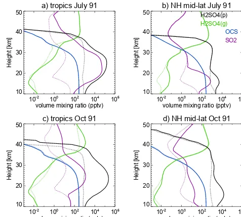
Figure 3. Volume mixing ratios of various sulfur containing species
(pptv) in the tropics (20◦S–20◦N, left) and NH mid-latitudes (35– 60◦N, right) during July 1991 (top) and October 1991 (bottom). Gas phase and particle phase H2SO4ratios are shown with green
and black lines, respectively. OCS and SO2are shown with blue and
purple lines, respectively. Runs A_Control20 and C_noPinatubo are shown with solid and dashed lines, respectively.
Also, A_Control20 has a peak stratospheric aerosol burden of 9.3 Tg at about day 260, but the aerosol burden from B_Control10 peaks around a month earlier, at around day 230, with 5.25 Tg of sulfur, which closely matches the HIRS observations. For A_Control20 and B_Control10, we find around 6.1 Tg and 3.5 Tg of sulfur by June 1992 (12 months after the eruption, day 530, day 530, first vertical dashed line in Fig. 2), suggesting e-folding timescales of 19 and 24 months, respectively. The shorter removal timescale for the 20 Tg run is likely due to the particles growing to larger sizes compared to the 10 Tg run (e.g. as seen in Fig. 8), and therefore sedimenting faster, moving to altitudes closer to the tropopause, where removal from the stratosphere is more effective. We note that, despite the close agreement be-tween the A_Control10 and the HIRS-derived burdens, the timescale estimates are considerably longer than values cited in the literature which range from around 12 to 14 months (e.g. see Baran and Foot, 1994 and Bluth et al., 1997).
4.3 Perturbation in sulfur species
October 1991, selected to correspond to the 15–45 day post-eruption period when the SO2is oxidised to H2SO4vapour, and approximately when the peak global aerosol burden oc-curs in the model. The profile of OCS shows the expected shape, being constant in the troposphere and then reducing with increasing altitude in the stratosphere as it is photol-ysed. The SO2profile from run C_noPinatubo shows a sharp reduction with height across the tropopause but then reaches a minimum and begins to increase with height to a local maximum at 30 km corresponding to where the source from OCS photolysis is largest. Below 30 km the sulfuric acid vapour follows a similar shape as SO2(but at lower concen-trations) but above that altitude continues to increase up to about 40 km. Below 35 km, the vertical profile of P-H2SO4 is approximately constant in the tropics in these quiescent conditions, but has a slight decrease with altitude. In the upper-middle stratosphere rapidly evaporating particles re-lease their H2SO4to the gas phase causing a sharp reduction in P-H2SO4about 40 km.
In the tropics, the July profiles from run A_Control20 (Fig. 3a) show large changes in concentrations of SO2and P-H2SO4(between 20 and 30 km) relative to run C_noPinatubo increasing by factors 103–104 and factor 102, respectively. The enhanced P-H2SO4 profile indicates that much of the SO2has already been oxidised and condensed into the par-ticle phase. By contrast, the NH mid-latitude July profiles show that the Pinatubo plume has not yet been transported, with SO2and aerosol H2SO4still at quiescent concentrations over almost the entire stratosphere, although some perturba-tion can be observed in the lowermost stratosphere and up-permost troposphere. It is notable that balloon-borne particle concentration soundings at Laramie (41◦N) in July 1991
al-ready show some enhanced layers between 15–18 km (Desh-ler et al., 1992) which corresponds well with the altitude of the SO2 and P-H2SO4 enhancement seen in the July-mean NH mid-latitude profiles.
The October mean SO2 profile is still strongly enhanced (factor 100) in the tropics with the P-H2SO4 enhancement only slightly higher than in July but over a much deeper layer. This tropical enhancement in both SO2and P-H2SO4 propagates up to about 40 km, and above that only the SO2 profiles show differences between runs A_Control20 and C_noPinatubo. It is interesting that the October 1991 trop-ical gas phase H2SO4profile from run A_Control20 actually shows lower values than in run C_noPinatubo in the main part of the plume (15–30 km), due to the condensation sink to aerosol being so much stronger. By contrast, above 30 km the increase in vapour pressure shuts off the condensation sink leading to the H2SO4 vapour concentrations being higher than quiescent at those altitudes. The October 1991 NH mid-latitude SO2and P-H2SO4profiles show only moderate en-hancement, suggesting that the easterly phase of the QBO has prevented transport of Pinatubo-enhanced air masses.
4.4 Stratospheric aerosol optical depth (sAOD) comparison
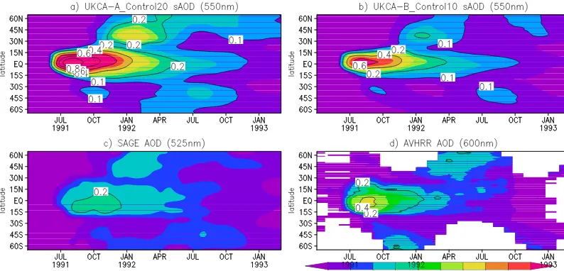
Figures 4a and b show the time evolution of the model mid-visible sAOD from runs A_Control20 and B_Control10 while Fig. 4c and d show the mid-visible sAOD measured by SAGE II and derived from AVHRR. Since AVHRR is a nadir viewing instrument, in Fig. 4d we have subtracted monthly-mean total AODs for the year prior to the eruption, matching the procedure recommended by Long and Stowe (1994) and used by Aquila et al. (2012). Note that the SAGE-II-derived sAOD is much lower than AVHRR in the trop-ics during the very high loading period after Pinatubo due to the measured extinction saturating at values above about 0.01 km−1 (Hamill et al., 2006). In both the A_Control20 and B_Control10 runs there is good qualitative agreement with the satellite regarding spatial and temporal distribution. For example, there is high sAOD after the eruption centred around the equator with peak sAOD in September 1991 in both model simulations and in the two satellite data sets. However, the model feature is narrower, confined between 10◦N and 10◦S. Another well-captured feature in the model is that there is no significant enhancement of sAOD in NH mid- and high latitudes until October 1991.
However, consistent with Fig. 2 (more aerosol loading than estimated by Baran and Foot, 1994) the simulated sAOD in A_Control20 is much larger than both sets of observations. The sAOD distribution in B_Control10 is in better agree-ment with the satellite measureagree-ments, comparing well to both satellite measurements in mid- and high latitudes. Compar-ing to the observed sAOD enhancements in the SH, both model simulations are also in quite good qualitative agree-ment. However, in the tropics the sAOD in B_Control10 is still about 50 % larger than that derived from AVHRR, and a factor of 2 larger than SAGE II. Possible causes for these biases are discussed later in this section.
4.5 Extinction comparison
Extinction profile measurements from SAGE II between July and September show (e.g. McCormick et al., 1995) that trans-port to the SH occurred mostly above about 24 km altitude. Aquila et al. (2012) highlighted the importance of resolving the enhanced tropical upwelling which occurred due to the long-wave absorption by the relatively larger stratospheric aerosol after the Pinatubo eruption. As explained in Sect. 2, in these simulations we do not radiatively couple the simu-lated aerosol with the model dynamics, and yet we capture quite well the SH post-Pinatubo sAOD evolution. We note that Aquila et al. (2012) do not include evaporation of sulfu-ric acid in their model, which could play an important role in influencing transport to SH mid-latitudes.
Figure 4. Time series of model-simulated zonal mean sAOD at 525 nm (calculated by integrating the extinction above the tropopause) for
runs (a) A_Control20 and (b) B_Control10. (c) and (d) show the sAOD measured by SAGE II (525 nm) and derived from AVHRR (600 nm) measurements. AVHRR sAOD is derived as the difference from the background total AOD from the 2 years before the eruption (Long and Stowe, 1994).
tropics (20◦S–20◦N). We choose these altitudes to allow comparison with the evaluation presented in Weisenstein et al. (2006, Fig. 6.20) for other stratospheric aerosol models. We compare extinction in the mid-visible (left panels) as well as the near-infrared (right panels). Here we use the updated v7.0 SAGE II data set and the profiles shown are averages between 20◦S and 20◦N. Monthly mean observed values are
calculated based on both sunrise and sunset profiles. At 20 and 25 km, both runs (A_Control20 and B_Control10) capture the general evolution of the trop-ical mid-visible extinction (Fig. 5), with the magnitude and timing of peak values, and the decay timescale, agreeing well with SAGE II. However, before the eruption (background conditions), modelled extinctions have a moderate low bias of 20–50 % at these levels. For the tropical mid-visible ex-tinction time series, run B_Control10 is in better agreement with the observations than A_Control20, which tends to be high biased (consistent with the sAOD and aerosol mass high biases seen in Figs. 2 and 4 respectively). However, against the tropical near-infrared extinction, run A_Control20 is in better agreement, with run B_Control10 generally showing modest low bias, although still in reasonable agreement. At 25 km, and for both wavelengths, the model tropical extinction peaks in August 1991, whereas in the satellite measurements, values plateau for 2–3 months before the decay period begins. In the model, the decay is fastest in the first 6–8 months after the peak value, with an approximately constant e-folding timescale from mid-1992 onwards. The faster decay in the early phase may be due to the shift in size distribution which produced larger particles at this time. Faster sedimentation would remove larger particles during this initial period, with the remaining (smaller on
average) particles sedimenting more slowly. Larger model high bias is seen for simulated tropical extinctions at 32 km, for both the runs (A_Control20 and B_Control10) that may indicate that the upper altitude used for SO2 injection was too high. At 32 km, the modelled extinction is slightly larger than SAGE II and, although peaks and troughs are mostly similar to the satellite measurements, the model variability is less than in the observations. We note again that the simulations presented here do not include the dynamical effects of aerosol-induced radiative heating. Such a radiative heating is known to cause increased tropical upwelling, which would cause greater dilution, could alter horizontal transport through the subtropical barrier and may also alter microphysical processes such as evaporation and coagulation.
10-6
10-5
10-4
10-3
10-2
10-1
ext [km-1]
SAGE II (525nm) A_Control20 B_Control10 C_noPinatubo Tropics (550nm) 32km
10-6
10-5
10-4
10-3
10-2
10-1 Tropics (1020nm)
32km
10-6
10-5
10-4
10-3
10-2
10-1
ext [km-1]
25km
10-6
10-5
10-4
10-3
10-2
10-1 25km
1990 1991 1992 1993 1994 1995 1996 10-6
10-5
10-4
10-3
10-2
10-1
ext [km-1]
20km
1990 1991 1992 1993 1994 1995 1996 10-6
10-5
10-4
10-3
10-2
[image:12.612.132.457.62.307.2]10-1 20km
Figure 5. Comparison between modelled and SAGE II (V7.0) retrieved extinction at 525 nm (left) and 1020 nm (right) in the tropics (20◦S– 20◦N) for 20 km (bottom), 25 km (middle) and 32 km (top). Extinctions from runs A_Control20, B_Control10 and C_noPinatubo are shown with red, orange and blue lines, respectively. The vertical black lines show the range of plus or minus one standard deviation over the individual measurements used in the calculation of the monthly mean.
10-6
10-5
10-4
10-3
10-2
10-1
ext [km-1]
SAGE II (525nm) A_Control20 B_Control10 C_noPinatubo NH mid-lat (550nm) 32km
10-6
10-5
10-4
10-3
10-2
10-1 NH mid-lat (1020nm)
32km
10-6
10-5
10-4
10-3
10-2
10-1
ext [km-1]
25km
10-6
10-5
10-4
10-3
10-2
10-1 25km
1990 1991 1992 1993 1994 1995 1996 10-6
10-5
10-4
10-3
10-2
10-1
ext [km-1]
20km
1990 1991 1992 1993 1994 1995 1996 10-6
10-5
10-4
10-3
10-2
10-1 20km
Figure 6. Same as Fig. 5 but for NH mid-latitudes (35–65◦N).
the simulations submitted for the Pinatubo intercomparison in SPARC (2006). Interestingly, differences between runs A_Control20 and B_Control10 are much smaller at this lati-tude band than in the tropics (Fig. 5), suggesting a larger
[image:12.612.134.457.378.621.2]1
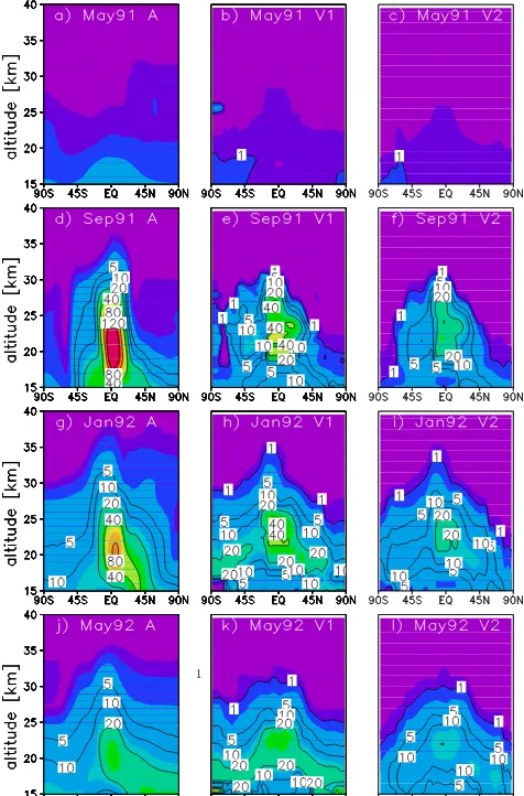
Figure 7. Comparison between zonal mean modelled (run
A_Control20) and satellite-derived V1 and V2 SAD (µm2cm−3) from SPARC (2006) and Arfeuille et al. (2013), respectively, for various months before and after the eruption.
20 km, the 1020 nm extinction from run A_Control20 shows better agreement with SAGE II than B_Control10.
4.6 Surface area density comparison
Figure 7 compares the vertical and latitudinal distribution of zonal mean SAD from run A_Control20 against two ver-sions of the satellite-derived SAD data set, for 4 selected months between May 1991 and May 1992. Before the erup-tion (May 1991), the model captures the global SAD distri-bution reasonably well compared to the SAGE-derived data sets, although model values are higher in the upper tropo-sphere and lower stratotropo-sphere (UTLS) region. For Septem-ber 1991 (3 months after the eruption), although the simu-lated SAD distribution broadly matches the observed shape, it is up to a factor 2 to 3 high in the tropics. Also, the model Pinatubo-enhanced SAD plume is strongly confined to the tropical pipe, whereas in the satellite-derived SAD (Fig. 7d)
one can see weak meridional transport to NH and SH sub-tropics at about 20–22 km. Young et al. (1994) showed that including the aerosol radiative effects on the model dynamics broadens the latitudinal extent of the Pinatubo cloud which, in our simulations would improve agreement with the satel-lite observations. And as mentioned earlier, such a heating can alter local circulation and may partially explain the SAD high biases seen here. By January 1992, the model high bias has reduced to a factor of 2, and the model shows meridional transport to NH mid-latitudes in the lowermost stratosphere, also seen in the observations. However, the satellite-derived SAD suggests meridional transport also occurs to the SH, but at slightly higher altitudes. By May 1992, high biases in modelled SAD are much smaller and the general latitu-dinal and altitulatitu-dinal distribution is still in good qualitative agreement with the observations, aside from the continued low bias in the SH. Also, as observed in Fig. 2 (younger age-of-air), in the lowermost stratosphere, the model seems to have too much diffusion near the tropopause. Hence the dis-tinct cross-tropopause gradients seen in satellite data are not seen in our simulations.
While interpreting the model–observation SAD discrep-ancies, one should consider how the satellite SAD product is derived from the SAGE I, SAGE II, SAM II (Stratospheric Aerosol Instrument II) and SME (Solar Mesosphere Ex-plorer) measurements. As noted earlier, the extinction mea-sured by the SAGE and SAM instruments has an upper limit of 0.01 km−1, above which the atmosphere is effectively opaque to the instruments (Hamill et al., 2006). During the peak aerosol loading period, when the model SAD is a factor of 2 high biased, it is apparent (for example in Fig. 5) that the SAGE II 525 nm and 1020 nm extinctions in the tropi-cal lower stratosphere are saturating at the upper limit value, with actual extinction values likely to have been higher. The late-1991 to 1992 period was flagged as missing data in the original SAGE II extinction data set. The data gaps during that period were addressed by Hamill et al. (2006), who used lidar data from two tropical sites (Camaguey, Cuba and Mauna Loa, Hawaii) and two mid-latitude sites (lidar from NASA Langley, Virginia, USA and backscatter sonde from Lauder, New Zealand), to fill the missing data.
4.7 Effective radius comparison
Another product derived from the gap-filled satellite extinc-tion record, that can be used to assess the evoluextinc-tion of the stratospheric aerosol properties following the Pinatubo erup-tion, isReff, defined as the ratio of the third and second inte-gral moments in radius, and which for multimodal distribu-tion can be represented as (Russell et al., 1996, Eq. 6)
Reff=
Pm
i=1Nirgi3 exp9/2(lnσi)2
Pm
i=1Nirgi2 exp2(lnσi)2
. (1)
The two gap-filled SAGE/SAM extinction data products provide 3-D time-varying volume concentration and SAD which together give Reff throughout the Pinatubo period. This record therefore has the potential to provide informa-tion on how the particle size distribuinforma-tion in the stratosphere was perturbed by the eruption. However, again, when com-paring the model to the satelliteReff, the limitations associ-ated with the derived product need to be considered. In par-ticular, because of the “blind spot” associated with particles smaller than 50–100 nm, Hamill et al. (2006) state that since the derived SAD may have an inherent low bias (whereas the derived volume density will be less affected) the derivedReff may overestimate the true value.
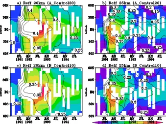
Figure 8 shows the evolution of the model zonal-meanReff at 20 and 25 km from runs A_Control20 and B_Control10 compared to that derived by Bauman et al. (2003) from the SAGE II and CLAES satellite measurements. The gen-eral spatial and temporal evolution of the model Reff is in good qualitative agreement with the observations in both runs, with values at 20 km larger than at 25 km, likely due to sedimentation. In the tropics, at both altitudes, the ob-servations suggest that, whereas sAOD and extinction are decaying by November or December 1991 (Figs. 4 and 5), the effective radius peaks several months later (early 1992) with only a slow decay beginning later in 1992. By contrast, in NH mid-latitudes, the observations suggest that the de-cay in effective radius is slightly earlier and occurs faster. Both simulations capture the timing of theseReffpeaks well, although at 25 km, the model peak is later than observed, matching the timing at 20 km. Effective radius values are always higher in the tropics than at mid-latitudes, a feature that is consistent between the model and observations. How-ever, althoughReff from run A_Control20 is slightly larger than from B_Control10, modelled values are up to 30–40 % smaller than those derived from the satellite, with maximum model Reff of around 0.4 and 0.35 µm, compared to around 0.6 µm from the satellites.
At 20 km (Fig. 8b), despite combining the two sets of satel-lite products, there is no observational constraint on the trop-icalReffbetween approximately June 1991 and August 1992, but the overall shape suggests theReffwas likely even larger than 0.6 µm during that period. The model low bias inReff is apparent at about the same extent at all latitudes and
alti-tudes and before the eruption, which suggests that it is not associated with sedimentation, since that would be expected to occur mostly during the highest loading period. There ap-pears to be a more persistent bias in simulated particle size distribution, but it is unclear whether the model has too many small particles, or too few large particles.
4.8 Particle size distribution
To give a stronger observational constraint on the simulated size distribution, we compare the model against balloon-borne CNC and OPC measurements made at Laramie, Wyoming, USA (41◦N, see Sect. 3). Figures 9 and 10 com-pare model profiles of size-resolved number concentrations (larger than a given particle diameter) against those mea-sured by the CNC and OPC. In each case we are com-paring a monthly-mean size-resolved particle concentration from the model to a single balloon sounding. Note also that whereas the number concentration profiles for particles larger than 5 nm, 150 nm and 250 nm are exactly as measured by the OPC, for the larger size channels we have interpolated the observations (linearly in logNvs. logRspace) onto reg-ularDp>550 nm, 750 nm and 1000 nm size channels from the irregular size thresholds given in the individual sounding data files.
Figure 8. Satellite-derived (shaded, from Bauman et al., 2003) and modelled (contours) effective radii (Reff) in µm at 25 and 20 km from
runs A_Control20 (panels a and b) and B_Control10 (panels c and d).
N5between 20 and 25 km. The observations show that con-centrations of particles at 150 nm and larger reduce sharply above 25 km, whereas the model profiles show only moder-ate decline. This suggests that the simple approach to particle evaporation may need improving.
For November 1991, the run A_Control20 shows enhance-ment up to 25 km for all the particle size thresholds, with the coarse mode higher than the run C_noPinatubo in the low-ermost stratosphere (not shown) and the shape of the verti-cal profile for each channel compares well with the obser-vations. The model also shows an enhanced layer of N5,
N150 and N250 at about 35km, suggesting transport of the Pinatubo plume to mid-latitudes throughout the lower and middle stratosphere. In both the model and observations, in these initial months, there is a layer where the N5 and
N150lines come together, reflecting that few particles remain smaller than 150 nm and indicating that particle growth at these sizes is strongest in that part of the stratosphere. We note however that in the observations this confluence occurs at around 20 km, whereas in the model this occurs around 16–17 km. This discrepancy in altitude could be reflecting the chosen injection height range, or be related to transport deficiencies in the model, and the general good qualitative agreement with the observations suggests that the modal ap-proach to aerosol dynamics is capturing the evolution of the size distribution rather well.
In order to evaluate the model size distribution profile in quiescent conditions, we compare to the Laramie balloon measurements in March 1991 (Fig. 10a). We then probe the
shown to be important by Saunders et al. (2012) and Brühl et al. (2013) or underestimated H2SO4photolysis rates in our simulations.
In March 1992 (Fig. 10b), 9 months after the eruption, the observed particle concentration profiles show major en-hancements throughout the upper troposphere and lower stratosphere (10 to 25 km), for size channels 150 nm and larger. By contrast, N5 shows a slight decrease compared to March 1991, and is only marginally higher than N150 and N250 for this month, suggesting that a large propor-tion of the particles have grown to sizes larger than 250 nm. The enhanced profiles ofN550,N750andN1000 are approx-imately constant between 15 and 20 km with a fast decrease at higher altitudes. Model run A_Control20 (solid line) cap-tures this volcanically enhanced particle size distribution re-markably well, with good qualitative and quantitative agree-ment across all the size channels in the main part of the plume. Run B_Control10 (dashed line) also captures well the
N5,N150andN250profiles, but is low biased in the larger size channels. Despite generally very good agreement with the Laramie OPC data at this time, in the lowermost stratosphere and upper troposphere (between 10 and 15 km), both model runs show a high bias in N150 andN250. We saw from the previous comparisons that run A_Control20 has too high a burden in the stratospheric aerosol compared to the HIRS and ISAMS satellite measurements (Fig. 2) and that it is strongly biased high in aerosol optical depth against the SAGE II and AVHRR data (Fig. 4). The comparisons to the OPC data sug-gest that the high sAOD bias originates from the overpre-dicted particle concentrations in the 150 to 550 nm radius range in the lowermost stratosphere, with coarser particles in that part of the atmosphere in reasonable agreement (run A_Control20) or showing low bias (run B_Control10).
In March 1993 (Fig. 10c), the observations show clear separation between N5 andN150, although N150 andN250 are close together. This indicates the formation of a bimodal size distribution consisting of an external mixture of particles which have grown to larger sizes following condensation af-ter oxidation of volcanic SO2and a separate sub-population of particles less influenced by the eruption. Observed pro-files of N550, N750 andN1000 show peak values at around 12km at this time, much lower altitudes than at March 1992 (Fig. 10b). It is interesting that the March 1993 N550 and
N750 profiles are higher in the 10–15 km region than in March 1992, likely indicating that, although slow at these particle sizes, sedimentation is transporting the particles to lower altitudes over these longer timescales. The model cap-tures the observed size distribution fairly well, withN250in quite good agreement with the measurements. However, the modelN150profile has a high bias of around a factor of 2 dur-ing March 1993 and is still together with theN5profile be-tween 15 and 20 km. Also, simulated particle concentrations in the larger size channels have a strong low bias of around a factor of 10 (run A_Control20) or 20 (run B_Control10) in the lowermost stratosphere at this time, with the
simu-lated profiles not capturing the increase in particles larger than N550 in the lowermost stratosphere. By March 1994 (Fig. 10d) the OPC measurements show that there has been a general decay in all size channels towards background con-ditions. The modelN150 high bias seen in March 1993 has worsened with the decay rate at these channels slower than in the observations. In theN550,N750andN1000channels, the model continues to have a low bias in both simulations. It is notable that throughout the period, the modelN150andN250 profiles are remarkably similar between the A_Control20 and B_Control10 simulations, with much larger differences in the coarser sized particles.
5 Discussion
In Sect. 4.2 we found that injecting 20 Tg SO2into the tropi-cal stratosphere substantially overestimates the stratospheric aerosol sulfur burden, with a 10 Tg SO2 injection in much better agreement with observations. Most previous modelling studies of the Pinatubo eruption have also tended to inject 20 Tg of SO2, and we show here that the high bias in our model is also found in other studies. Oman et al. (2006) and English et al. (2013) found peak stratospheric sulfuric acid aerosol burdens of 27 and 24 Tg respectively, translating to 36 and 32 Tg aerosol mass assuming 75 % weight sulfuric acid, similar to our 37 Tg peak value. Niemeier et al. (2009) injected 17 Tg of SO2, and their 30 Tg peak stratospheric aerosol burden also agrees with our simulation, accounting proportionally for the reduced sulfur source. We note also that Niemeier et al. (2009) and English et al. (2013) have presented the HIRS stratospheric aerosol burden time series from Baran and Foot (1994) assuming the mass burden is for sulfuric acid, without accounting for the fraction of water content implicit in those values.
For our 10 Tg Pinatubo simulation, we found generally good agreement with observed sAOD (section 4.4), extinc-tion (secextinc-tion 4.5), and SAD (secextinc-tion 4.6). Our 20 Tg simu-lation gives consistently too high sAOD in the tropics, mid-latitudes and polar regions, whereas in most of the previous studies mentioned above, reasonable agreement is found in peak AOD, despite the high bias in stratospheric aerosol bur-den. We note however that there is a considerable diversity in the injection height-range, latitudinal spread and duration of the volcanic source used in these different model experi-ments.
Figure 9. August, September, October, November 1991 profiles of size-resolved number concentrations of particles (cm−3) with radii larger than 5, 150, 250, 550, 750 and 1000 nm from Laramie (41.3◦N, 105.5◦W) are shown with plus (+) symbol. Solid and dashed lines show aerosol profiles from the runs A_Control20 and B_Control10, respectively, highlighting the region where the model predicts perturbation in the aerosol profiles. Horizontal coloured lines represent standard deviations (1σ) in number concentrations for a given month calculated from daily values for run A_Control20.
Figure 10. Same as Fig. 9 but for March 1991, March 1992, March 1993 and March 1994.
a largerReffwill have caused important changes in the radia-tive properties of the stratospheric aerosol, with significant absorption of outgoing terrestrial radiation and a decrease in
[image:17.612.125.469.389.636.2]dynamics in stratospheric CCMs, and we aim to include and assess the impact of these feedbacks in a future study (Mann et al., in prep., 2014).
Our simulations here indicate that the model is capable of capturing the main features of the observed evolution of the particle size distribution very well, with particularly good agreement with the measurements in the most perturbed post-eruption period through to mid-1992. However, Fig. 10c and d suggest that the decay phase is not well captured, withN150 reducing much more slowly than the measurements and the return to a background size distribution occurs much later in the model. We have seen that simulated particle concen-trations in the 5–250 nm size range, whilst agreeing well in background conditions, have moderate high bias in the first year after the eruption, with the bias worsening as the model decays too slowly in the subsequent period. There are sev-eral possible causes for this model size distribution bias. It could be that the simplified modal representation of aerosol dynamics may be only partly capturing the different parti-cle growth and removal rates across the partiparti-cle size range. However, it is also worth noting that the largest biases oc-curred in the lowermost stratosphere and upper troposphere where STE-related processes may not be well captured in our low-resolution GCM. Another related issue is that we again note that these simulations do not include the coupling to dy-namics which would increase the altitude of the aerosol layer and reduce concentrations in the lower part of the plume, where the high bias is mostly evident. Also, our model has too young age-of-air in mid-latitudes (see Fig. 1d) which may also be affecting the simulated transport and particle size evolution. Finally, we also note that nucleation rates at the very low humidity and temperature conditions in the strato-sphere are known to be highly uncertain. The Vehkamäki et al. (2002) parameterisation used in this paper is the best available for stratospheric conditions, but is essentially an extrapolation from laboratory measurements at much higher temperatures and humidities, based on classical nucleation theory.
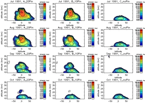
Our study is the first to fully examine the variation in sim-ulated particle size distribution through the Pinatubo post-eruption period, and we therefore choose to document the nu-cleation rate occurring in our simulations. Figure 11 shows, for runs A_Control20, B_Control10 and C_noPinatubo, the zonal-mean nucleation rate against latitude and altitude for monthly means through August to October 1991. In volcani-cally quiescent conditions (C_noPinatubo), the model has nucleation occurring mainly in the tropical upper troposphere with negligible new particle formation in the stratosphere. Note that the observed and simulated lower stratosphericN5 andN150profiles at Laramie in March 1991 (Fig. 10a) are in very good agreement, and Fig. 11 indicates that these strato-spheric particles were actually formed in the tropical upper troposphere, consistent with the stratospheric aerosol lifecy-cle described by Hamill et al. (1997). The observations at Laramie indicate that only a small proportion of these
nu-cleated particles grow to sizes larger than 150 nm, with most remaining at smaller sizes. We note however that nucleation can be seen in the middle stratosphere at SH mid-latitudes in the volcanically quiescent C_noPinatubo September 1991 monthly-mean, indicating the occurrence of nucleation in springtime, as seen in the McMurdo OPC record (Campbell and Deshler, 2014). Note that the mechanism here is that par-ticle evaporation and subsequent photolysis of sulfuric acid leads to a reservoir of SO2building up during polar winter, which leads to new particle formation in polar spring (Mills et al., 2005). This is the same mechanism that is leading to the layer of elevatedN5at 25–30 km in the March Laramie profiles (see Fig. 10).
Figure 11 suggests that, following Pinatubo, strong nu-cleation occurred throughout the injection height range of 19–27 km for around 6 weeks after the eruption. Although twice as much SO2 is injected in A_Control20 than in B_Control10, the nucleation rates in the two runs are simi-lar for July 1991. This could possibly be indicative of a de-pletion of oxidants which is limiting SO2oxidation at this time, although an alternative explanation might be that there is much more surface area in the 20 Tg injection run to act as a condensation sink for sulfuric acid vapour. Nucleation rates then reduce in magnitude through August and Septem-ber as the emitted SO2 is completely converted to sulfuric acid and there is a substantial surface area to provide a con-densation sink of H2SO4. By October 1991, nucleation rates in A_Control20 and B_Control10 have returned to similar values to those found in the quiescent C_noPinatubo simu-lation. Following the eruption of Mount Pinatubo, the bal-loon observations at Laramie indicate that, by March 1992 (e.g. Fig. 10b),N150is increased by a factor of 8, whereasN5 has already returned to pre-eruption values, consistent with the reduced nucleation rate seen here. As a consequence,N5 andN150profiles are separated by only a few tens of percent, indicating that the majority of particles in the lower strato-sphere have grown larger than 150 nm at that time. This fea-ture was well capfea-tured by the model in runs A_Control20 and B_Control10 with theN5,N150andN250profiles being remarkably similar between the two runs.
Figure 11. Modelled nucleation rates (cm3s−1) from runs A_Control20 (left), B_Control10 (middle), and C_noPinatubo (right) for (top to bottom) July, August, September and October 1991.
part of the plume (28 to 30 km). However, the accumulation mode SAD fraction (Fig. 12c) shows that even during the early phase of eruption total SAD is primarily determined by these larger particles in the lower–middle stratosphere. At a later stage (December 1991, not shown), the contribution from nucleation and Aitken mode is insignificant and, as ex-pected, the accumulation mode then contributes the vast ma-jority of the SAD. We note that in Fig. 7 the model shows highest biases in simulated SAD against the observations during the first few months after the eruption.
Figure 13 compares tropical (panel a) and global (panel b) mid-visible sAOD andN150 evolution from the three main simulations A_Control20, B_Control10 and C_noPinatubo against the satellite observations from AVHRR. We also compare time series of simulatedN150 at 18 and 22 km al-titude against the long time series OPC measurements from Laramie. Also presented in Fig. 13 are results from two additional 10 Tg simulations, designed to test the sensitiv-ity of the model predictions to sub-grid particle formation (run D_noPrimary10) and with much reduced new particle formation rate (run E_ScaledStNuc10). Both of these